
Full Bayesian Significance Testing for Neural Networks in Traffic Forecasting
Proceedings of the Thirty-Third International Joint Conference on Artificial Intelligence. Main Track. Pages 2216-2224.
https://doi.org/10.24963/ijcai.2024/245
Keywords
- Machine Learning: ML: Explainable/Interpretable machine learning
- Uncertainty in AI: UAI: Uncertainty representations
- Knowledge Representation and Reasoning: KRR: Learning and reasoning
- Data Mining: DM: Mining spatial and/or temporal data
Abstract
Due to the complex and dynamic traffic contexts, the interpretability and uncertainty of traffic forecasting have gained increasing attention. Significance testing is a powerful tool in statistics used to determine whether a hypothesis is valid, facilitating the identification of pivotal features that predominantly contribute to the true relationship. However, existing works mainly regard traffic forecasting as a deterministic problem, making it challenging to perform effective significance testing. To fill this gap, we propose to conduct Full Bayesian Significance Testing for Neural Networks in Traffic Forecasting, namely ST-nFBST. A Bayesian neural network is utilized to capture the complicated traffic relationships through an optimization function resolved in the context of aleatoric uncertainty and epistemic uncertainty. Thereupon, ST-nFBST can achieve the significance testing by means of a delicate grad-based evidence value, further capturing the inherent traffic schema for better spatiotemporal modeling. Extensive experiments are conducted on METR-LA and PEMS-BAY to verify the advantages of our method in terms of uncertainty analysis and significance testing, helping the interpretability and promotion of traffic forecasting.
- [Ahmed and Cook, 1979] Mohammed S Ahmed and Allen R Cook. Analysis of freeway traffic time-series data by using Box-Jenkins techniques. 1979.
- [Atwood and Towsley, 2016] James Atwood and Don Towsley. Diffusion-convolutional neural networks. In NIPS, 2016.
- [Bai et al., 2020] Lei Bai, Lina Yao, Can Li, Xianzhi Wang, and Can Wang. Adaptive graph convolutional recurrent network for traffic forecasting. In NeurIPS, 2020.
- [Blei et al., 2017] David M Blei, Alp Kucukelbir, and Jon D McAuliffe. Variational inference: A review for statisti- cians. Journal of the American statistical Association, 112(518):859-877, 2017.
- [Blundell et al., 2015] Charles Blundell, Julien Cornebise, Koray Kavukcuoglu, and Daan Wierstra. Weight uncer- tainty in neural network. In ICML, 2015.
- [Cressie and Wikle, 2015] Noel Cressie and Christopher K Wikle. Statistics for spatio-temporal data. 2015.
- [De Braganc ¸a Pereira and Stern, 1999] Carlos Alberto De Braganc ¸a Pereira and Julio Michael Stern. Evidence and credibility: Full Bayesian significance test for precise hy- potheses. Entropy, 1(4):99-110, 1999.
- [Denker and LeCun, 1990] John Denker and Yann LeCun. Transforming neural-net output levels to probability dis- tributions. In NIPS, 1990.
- [Fan and Li, 1996] Yanqin Fan and Qi Li. Consistent model specification tests: omitted variables and semiparametric functional forms. Econometrica: Journal of the econo- metric society, pages 865-890, 1996.
- [Gal and Ghahramani, 2016] Yarin Gal and Zoubin Ghahra- mani. Dropout as a bayesian approximation: Representing model uncertainty in deep learning. In ICML, 2016.
- [Gehring et al., 2017] Jonas Gehring, Michael Auli, David Grangier, Denis Yarats, and Yann N Dauphin. Convolu- tional sequence to sequence learning. In ICLR, 2017.
- [Horel and Giesecke, 2020] Enguerrand Horel and Kay Giesecke. Significance tests for neural networks. Journal of Machine Learning Research, 21(227):1-29, 2020.
- [Ji et al., 2020] Jiahao Ji, Jingyuan Wang, Zhe Jiang, Jing- tian Ma, and Hu Zhang. Interpretable spatiotemporal deep learning model for traffic flow prediction based on poten- tial energy fields. In ICDM, 2020.
- [Ji et al., 2023] Jiahao Ji, Jingyuan Wang, Chao Huang, Junjie Wu, Boren Xu, Zhenhe Wu, Junbo Zhang, and Yu Zheng. Spatio-temporal self-supervised learning for traffic flow prediction. In AAAI, 2023.
- [Jiang and Luo, 2022] Weiwei Jiang and Jiayun Luo. Graph neural network for traffic forecasting: A survey. Expert Systems with Applications, 207:117921, 2022.
- [Jiang et al., 2023a] Jiawei Jiang, Chengkai Han, Wayne Xin Zhao, and Jingyuan Wang. Pdformer: Propagation delay- aware dynamic long-range transformer for traffic flow pre- diction. In AAAI, 2023.
- [Jiang et al., 2023b] Jiawei Jiang, Dayan Pan, Houxing Ren, Xiaohan Jiang, Chao Li, and Jingyuan Wang. Self- supervised trajectory representation learning with tempo- ral regularities and travel semantics. In ICDE, 2023.
- [Jiang et al., 2023c] Wenjun Jiang, Wayne Xin Zhao, Jingyuan Wang, and Jiawei Jiang. Continuous trajectory generation based on two-stage gan. In AAAI, 2023.
- [Kendall and Gal, 2017] Alex Kendall and Yarin Gal. What uncertainties do we need in bayesian deep learning for computer vision? In NIPS, 2017.
- [Kipf and Welling, 2017] Thomas N Kipf and Max Welling. Semi-supervised classification with graph convolutional networks. In ICLR, 2017.
- [Lakshminarayanan et al., 2017] Balaji Lakshminarayanan, Alexander Pritzel, and Charles Blundell. Simple and scal- able predictive uncertainty estimation using deep ensem- bles. In NIPS, 2017.
- [Lavergne and Vuong, 1996] Pascal Lavergne and Quang H Vuong. Nonparametric selection of regressors: The nonnested case. Econometrica: Journal of the Economet- ric Society, pages 207-219, 1996.
- [Lavergne and Vuong, 2000] Pascal Lavergne and Quang Vuong. Nonparametric significance testing. Econometric Theory, 16(4):576-601, 2000.
- [Li and Zhu, 2021] Mengzhang Li and Zhanxing Zhu. Spatial-temporal fusion graph neural networks for traffic flow forecasting. In AAAI, 2021.
- [Li et al., 2018] Yaguang Li, Rose Yu, Cyrus Shahabi, and Yan Liu. Diffusion convolutional recurrent neural net- work: Data-driven traffic forecasting. In ICLR, 2018.
- [Liu et al., 2023] Hao Liu, Wenzhao Jiang, Shui Liu, and Xi Chen. Uncertainty-aware probabilistic travel time pre- diction for on-demand ride-hailing at didi. In SIGKDD, 2023.
- [Liu et al., 2024] Zehua Liu, Zimeng Li, Jingyuan Wang, and Yue He. Full bayesian significance testing for neural networks. In AAAI, 2024.
- [Ma et al., 2015] Xiaolei Ma, Zhimin Tao, Yinhai Wang, Haiyang Yu, and Yunpeng Wang. Long short-term mem- ory neural network for traffic speed prediction using re- mote microwave sensor data. Transportation Research Part C: Emerging Technologies, 54:187-197, 2015.
- [Ma et al., 2017] Xiaolei Ma, Zhuang Dai, Zhengbing He, Jihui Ma, Yong Wang, and Yunpeng Wang. Learning traf- fic as images: A deep convolutional neural network for large-scale transportation network speed prediction. Sen- sors, 17(4):818, 2017.
- [MacKay, 1992] David JC MacKay. A practical bayesian framework for backpropagation networks. Neural com- putation, 4(3):448-472, 1992.
- [Min and Wynter, 2011] Wanli Min and Laura Wynter. Real- time road traffic prediction with spatio-temporal correla- tions. Transportation Research Part C: Emerging Tech- nologies, 19(4):606-616, 2011.
- [Mori et al., 2015] Usue Mori, Alexander Mendiburu, Maite Álvarez, and Jose A Lozano. A review of travel time estimation and forecasting for advanced traveller infor- mation systems. Transportmetrica A: Transport Science, 11(2):119-157, 2015.
- [Neal, 1995] Radford M. Neal. Bayesian learning for neural networks. PhD thesis, University of Toronto, 1995.
- [Olden and Jackson, 2002] Julian D Olden and Donald A Jackson. Illuminating the "black box": a randomization approach for understanding variable contributions in arti- ficial neural networks. Ecological modelling, 154, 2002.
- [Qian et al., 2023] Weizhu Qian, Dalin Zhang, Yan Zhao, Kai Zheng, and JQ James. Uncertainty quantification for traffic forecasting: A unified approach. In ICDE, 2023.
- [Racine, 1997] Jeff Racine. Consistent significance testing for nonparametric regression. Journal of Business & Eco- nomic Statistics, 15(3):369-378, 1997.
- [Song et al., 2020] Chao Song, Youfang Lin, Shengnan Guo, and Huaiyu Wan. Spatial-temporal synchronous graph convolutional networks: A new framework for spatial- temporal network data forecasting. In AAAI, 2020.
- [Sutskever et al., 2014] Ilya Sutskever, Oriol Vinyals, and Quoc V Le. Sequence to sequence learning with neural networks. In NIPS, 2014.
- [Wang et al., 2014] Jian Wang, Wei Deng, and Yuntao Guo. New bayesian combination method for short-term traffic flow forecasting. Transportation Research Part C: Emerg- ing Technologies, 43:79-94, 2014.
- [Wang et al., 2018] Jingyuan Wang, Ze Wang, Jianfeng Li, and Junjie Wu. Multilevel wavelet decomposition network for interpretable time series analysis. In SIGKDD, 2018.
- [Wang et al., 2019a] Bin Wang, Jie Lu, Zheng Yan, Huaishao Luo, Tianrui Li, Yu Zheng, and Guangquan Zhang. Deep uncertainty quantification: A machine learning approach for weather forecasting. In KDD, 2019.
- [Wang et al., 2019b] Jingyuan Wang, Ning Wu, Wayne Xin Zhao, Fanzhang Peng, and Xin Lin. Empowering a* search algorithms with neural networks for personalized route recommendation. In SIGKDD, 2019.
- [Wang et al., 2021] Jingyuan Wang, Zhen Peng, Xiaoda Wang, Chao Li, and Junjie Wu. Deep fuzzy cognitive maps for interpretable multivariate time series prediction. IEEE Transactions on Fuzzy Systems, 29(9):2647-2660, 2021.
- [Wang et al., 2023a] Jingyuan Wang, Jiahao Ji, Zhe Jiang, and Leilei Sun. Traffic flow prediction based on spa- tiotemporal potential energy fields. IEEE Transactions on Knowledge and Data Engineering, 35(9), 2023.
- [Wang et al., 2023b] Jingyuan Wang, Chen Yang, Xiaohan Jiang, and Junjie Wu. When: A wavelet-dtw hybrid at- tention network for heterogeneous time series analysis. In SIGKDD, 2023.
- [White, 1989a] Halbert White. Learning in artificial neural networks: A statistical perspective. Neural computation, 1(4):425-464, 1989.
- [White, 1989b] Halbert White. Some asymptotic results for learning in single hidden-layer feedforward network models. Journal of the American Statistical Association, 84(408):1003-1013, 1989.
- [Wu et al., 2019] Zonghan Wu, Shirui Pan, Guodong Long, Jing Jiang, and Chengqi Zhang. Graph wavenet for deep spatial-temporal graph modeling. arXiv preprint arXiv:1906.00121, 2019. IJCAI
- [Wu et al., 2020a] Ning Wu, Xin Wayne Zhao, Jingyuan Wang, and Dayan Pan. Learning effective road network representation with hierarchical graph neural networks. In SIGKDD, 2020.
- [Wu et al., 2020b] Zonghan Wu, Shirui Pan, Guodong Long, Jing Jiang, Xiaojun Chang, and Chengqi Zhang. Con- necting the dots: Multivariate time series forecasting with graph neural networks. In SIGKDD, 2020.
- [Wu et al., 2021] Dongxia Wu, Liyao Gao, Matteo Chinazzi, Xinyue Xiong, Alessandro Vespignani, Yi-An Ma, and Rose Yu. Quantifying uncertainty in deep spatiotemporal forecasting. In SIGKDD, 2021.
- [Xu et al., 2020] Mingxing Xu, Wenrui Dai, Chunmiao Liu, Xing Gao, Weiyao Lin, Guo-Jun Qi, and Hongkai Xiong. Spatial-temporal transformer networks for traffic flow forecasting. arXiv preprint arXiv:2001.02908, 2020.
- [Ye et al., 2021] Junchen Ye, Leilei Sun, Bowen Du, Yanjie Fu, and Hui Xiong. Coupled layer-wise graph convolution for transportation demand prediction. In AAAI, 2021.
- [Yu et al., 2018] Bing Yu, Haoteng Yin, and Zhanxing Zhu. Spatio-Temporal Graph Convolutional Networks: A Deep Learning Framework for Traffic Forecasting. In IJCAI, 2018. IJCAI
- [Zhang et al., 2017] Junbo Zhang, Yu Zheng, and Dekang Qi. Deep spatio-temporal residual networks for citywide crowd flows prediction. In AAAI, 2017.
- [Zhang et al., 2019] Junbo Zhang, Yu Zheng, Junkai Sun, and Dekang Qi. Flow prediction in spatio-temporal net- works based on multitask deep learning. IEEE Transac- tions on Knowledge and Data Engineering, 32, 2019.
- [Zhou et al., 2021] Zhengyang Zhou, Yang Wang, Xike Xie, Lei Qiao, and Yuantao Li. Stuanet: Understanding un- certainty in spatiotemporal collective human mobility. In Proceedings of the Web Conference 2021, 2021.
References were extracted automatically from the PDF and may contain errors.
Full text extracted automatically from the PDF; figures, tables and equations may differ. The PDF is the version of record.
1 Introduction
With substantial amounts of daily traffic data, including flow, volume, and speed, collected via city sensors, Intelligent Transportation Systems (ITS) [Mori et al., 2015] have come to the forefront in meeting the mounting challenges presented by ever-increasing transportation network demands. Traffic forecasting, a core constituent of ITS, aims to extrapolate future traffic conditions based on historical data and existing road networks. Its crucial role spans across traffic management, planning, and control functionalities.
In traffic forecasting, earlier methods primarily depend on statistical models [Ahmed and Cook, 1979; Min and Wynter, 2011; Cressie and Wikle, 2015], albeit these are limited in deployment due to stringent data assumptions and constrained abilities to capture intricate non-linear correlations. In recent years, the advances of deep learning have significantly enhanced the task completion of current methods. They benefit from the powerful capabilities of Graph Neural Networks (GNNs) to extract spatial dependencies from graphs [Kipf and Welling, 2017; Jiang and Luo, 2022; Song et al., 2020; Xu et al., 2020] and the sequence learning techniques to capture temporal dependencies [Gehring et al., 2017; Wu et al., 2019; Bai et al., 2020; Li et al., 2018].
∗Corresponding author
Despite the considerable success achieved by existing methods in prediction performance, the considerations of interpretability and uncertainty in traffic forecasting have been consistently disregarded. The bulk of these methods merely provide deterministic predictions, failing to account for the essential factor of uncertainty. However, the spatial-temporal relationships found in traffic data exhibit a high degree of complexity and diversity. It frequently leads models to incorporate unstable correlations and noise information in data, subsequently resulting in erratic model performance. Therefore, understanding the inherent evolution schema in traffic forecasting and identifying the pivotal traffic factors become imperative. Furthermore, this comprehension forms the foundation for effectively optimizing the modeling of true relationships in traffic forecasting. Despite the growing concerns regarding the uncertainty of prediction results [Liu et al., 2023; Qian et al., 2023; Wu et al., 2021], the interpretability of traffic forecasting remains an unresolved challenge.
Significance testing is a powerful tool in statistics to tackle the problem. It aims to determine whether a proposition about the population distribution 1 is true or false given observations, which is widely used in many scientific fields. However, traditional significance testing is restricted by assumptions about the true relationship and the derivation of complicated, even intractable, theoretical distributions, thus imposing strict limitations on the model. Hence, significance testing in spatial-temporal forecasting predominantly relies on shallow models, such as ARIMA. Recently, [Horel and Giesecke, 2020] and [Liu et al., 2024] have successfully introduced neural networks into significance testing, yielding impressive results. However, there is a dearth of research on significance testing for deep learning in traffic forecasting.
To fill this gap, we propose to conduct Full Bayesian Significance Testing for Neural Networks in Traffic Forecasting, namely ST-nFBST. It is a Bayesian framework incorporating spatial-temporal modeling, uncertainty quantification, and significance testing. First, we approach traffic forecasting through Bayesian modeling and employ a Bayesian neural network to capture complicated traffic relationships. Then, the framework is optimized in the context of heteroscedastic aleatoric uncertainty and epistemic uncertainty, decomposing the prediction risks derived from the model and data, respectively. Thereby, a quantitative analysis of both uncertainties can be implemented. Finally, a delicate grad-based Bayesian evidence is calculated based on the posterior distribution of parameters, and the testing results would contribute to reconstructing input graph signals. Through the analysis of experimental results with real data, we have successfully identified the inherent schema that impacts traffic forecasting on marginal and central nodes from both temporal and spatial dimensions. Building upon this discovery, we optimize the traffic prediction model, significantly reducing both model uncertainty and prediction errors.
1 https://online.stat.psu.edu/stat462/node/249/
The main contributions can be summarized as follows:
- To the best of our knowledge, we are the first to capture the inherent evolution schema in traffic forecasting through significance testing for neural networks.
- We propose ST-nFBST, a Bayesian framework incorporating spatial-temporal modeling, uncertainties quantification, and significance testing. It effectively improves predictive performance while reducing uncertainty.
- ST-nFBST can effectively detect changes in traffic conditions through uncertainty analysis, identify the inherent traffic schema and provide guidance for reconstructing the input graph signals through significance testing.
- Extensive experiments are conducted to verify the advantages of our approach in terms of traffic forecasting and significance testing.
2 Preliminaries
In this section, we first introduce basic notations in this paper. Then, we formalize the problem of traffic forecasting.
2.1 Notations and Definitions
Definition 1 (Sensor Network). We represent the sensor network as a weighted directed graph G = (V, E,W), where V = {v1, . . . , v|V|} is a set of |V| nodes, each node vi representing a sensor, E ⊆ V × V is a set of edges, each ei,j = (vi, vj) representing the correlation between sensors vi and vj, and W ∈ R|V|×|V| is a weighted adjacency matrix representing the nodes proximity (e.g., a function of their road network distance).
Definition 2 (Traffic States). Denote the traffic states observed on G as a graph signal x = (x1, . . . , x|V|) ∈ R|V| , such as velocity, volume, and flow. Traffic states can be regarded as multivariate time series. In this context, x(t) denotes the graph signal observed at time t, representing the values obtained from all sensors in the sensor network at time t; x(t) i represents the value obtained from the i-th sensor in the sensor network at time t.
2.2 Problem Statement
Problem 1 (Traffic Forecasting). The goal of traffic forecasting is to predict the future traffic state given previously observed traffic states from |V| correlated sensors in the sensor network. Let X<t = {x(t-τ1+1) , . . . , x(t) } ∈ Rτ1×|V| be the corresponding historic input sequence with τ1 steps. Similarly, X>t = {x(t+1) , . . . , x(t+τ2) } ∈ Rτ2×|V| represents the prediction sequence, where τ2 denotes the prediction horizon. The traffic forecasting problem aims to learn a function f(·) that maps τ1 historical graph signals X<t to future τ2 graph signals X>t, given a graph G:
For convenience, we will simplify X<t as Xt and X>t as Y t in the following discussion.
3 Methodology
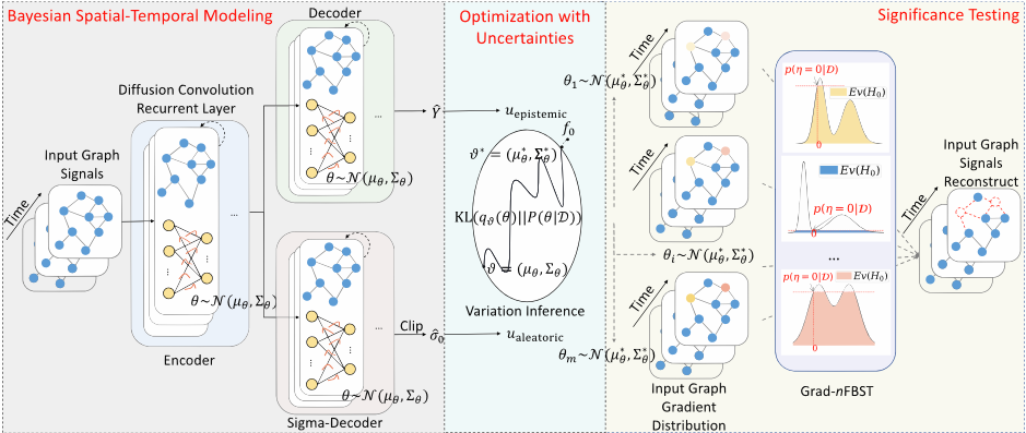
In this section, we introduce the proposed ST-nFBST framework (Figure 1). We start with the modeling of spatial and temporal dependencies in a Bayesian perspective. Then, we introduce the aleatoric uncertainty and epistemic uncertainty and formulate the optimization problem in the context of both uncertainties. Finally, we display how to conduct significance testing through a delicate grad-based evidence value.
3.1 Bayesian Spatial-Temporal Modeling
Instead of regarding traffic forecasting as deterministic, we model it from a Bayesian perspective. Given a dataset of n samples D = {(X1, Y 1), . . . , (Xn, Y n)}, we use a Bayesian neural network (BNN) [Denker and LeCun, 1990; MacKay, 1992; Neal, 1995], whose parameters θ follow a distribution rather than deterministic values, to represent the underlying function f0 : Rτ1×|V| → Rτ2×|V| . For a pair of observations (Xt, Y t) at time point t, the regression process can be modeled as corrupted with Gaussian random noise:
The Gaussian assumption is common and computationally stable for regression tasks [Lakshminarayanan et al., 2017; Kendall and Gal, 2017; Gal and Ghahramani, 2016]. We assume the observation noise can vary with inputs Xt at different time points, namely heteroscedastic. In traffic forecasting, the traffic state highly depends on complicated contexts, such as congestion, weather conditions, and unexpected traffic events, resulting in substantial variability. Consequently, heteroscedastic modeling is more aligned with real scenarios. Given a new case Xt, the prediction made by the Bayesian neural network is the weighted average of an ensemble
where Θ is the whole parameter space.
As shown in Figure 1, the architecture includes an encoder and two independent decoders, respectively modeling spatialtemporal dependencies and observation noise. We model the spatial dependency by relating traffic flow to a diffusion process, which explicitly captures the stochastic nature of traffic dynamics. The diffusion convolution operation over a graph signal x and a filter fθ is defined as [Li et al., 2018]
where k is the diffusion step, θ ∈ RK×2 is the parameter for the filter, and DOW,D-1 I W ⊤ represent the transition matrices of the diffusion process and the reverse one. Then, we leverage the Diffusion Convolutional Gated Recurrent Unit (DCGRU) [Li et al., 2018] to model the temporal dependency
Based on DCGRU and Sequence to Sequence architecture, we build an encoder and two independent decoders. They all adhere to BNNs and the random outputs of the model f are
where θ ∼ P(θ|D). Besides, we add a ReLU-like clip layer after the Sigma-Decoder to ensure that ˆσ0(Xt) is always positive. Specifically, ˆσ0(Xt) = max(ˆσ0(Xt), τ), where τ is the threshold to control the precision.
3.2 Optimization with Uncertainties
In Bayesian modeling, there exist two primary categories of uncertainty, i.e., aleatoric and epistemic. The former represents data uncertainty, while the latter represents model uncertainty. Our framework incorporates both uncertainties into the optimization of traffic forecasting.
Aleatoric Uncertainty. Aleatoric uncertainty is caused by the intrinsic randomness of data, which cannot be reduced even if more data were to be collected. For example, it could be caused by sensor noise inherent in the observations. Under the assumption of Eq (2), the aleatoric uncertainty is exactly equal to the variance of the noise
Epistemic Uncertainty. Epistemic uncertainty accounts for uncertainty in the model parameters, which arises from that lack of data or model misspecification. Fortunately, this uncertainty can be explained away given enough data. In traffic forecasting, the epistemic uncertainty can be captured by the predictive variance:
Before optimization, a prior distribution is assigned to model parameters θ as an initial belief π(θ) according to experience. This belief is gradually adjusted to fit data D by using the Bayesian rule. The final belief is presented as the posterior distribution
The main challenge of optimization lies in the difficulty of solving the integral in Eq (9) in practice. A popular way, known as Variational Inference (VI), entails approximating the real but intractable posterior distribution with a tractable distribution called variational distribution [Blei et al., 2017]. Therefore, Eq (9) could be efficiently approximated. Formally, variational family Q = {qϑ : ϑ ∈ Γ} is a predefined family of tractable distributions on model parameter space Θ, where ϑ is the parameter of variational distribution and Γ is the range of ϑ. The optimal variational distribution qϑ∗ is chosen from Q such that
KL divergence describes the "distance" between two distributions. We set diagonal Gaussian distributions as the prior and variational families of parameter θ. This assumption is common in many works [Blundell et al., 2015; Kendall and Gal, 2017]. Under this assumption, Eq (10) can be further simplified as (excluding the constant logP(D))
The first term is related to data, which is equivalent to Mean Squared Error (MSE) with a scaling factor 1 2σ2 0 under the assumption Eq (2). The second term is only related to parameters ϑ. The detailed derivation is shown in the Appendix.
In the end, we finish approximating the posterior distribution of parameters P(θ|D) with variational distribution qϑ∗(θ). Using Monte Carlo integration, the aleatoric uncertainty and epistemic uncertainty are approximated as follows:
where ˆσ0(Xt), ˆ Y t are the outputs of two decoders obtained by sampling m times drawn from θ ∼ qϑ∗(θ), respectively.
3.3 Significance Testing
To capture the traffic evolution schema, we propose to conduct significance testing in traffic forecasting. However, there are two main defects in classical significance testing.
- First, the effectiveness of classical significance testing is based on reasonable assumptions about f0, such as stationarity and invertibility (ARIMA). However, it is difficult to find such precise and suitable assumptions when the data distribution is complicated such as traffic forecasting.
- Second, some models, such as deep learning, excel in accurately fitting complex data distributions. However, the more complex the assumption of f0, the more computational derivation of theoretical distribution, which is inevitable for classical significance testing.
Fortunately, nFBST replaces complicated theoretical derivation by fitting distributions in a Bayesian way, and the neural network serves as a good estimator of f0 without assuming specific forms [Liu et al., 2024].
In traffic forecasting, to test the significance of input features Xt, we first need a reasonable measure as the testing statistic to represent the true relationship between features and targets. In this paper, we conduct the Bayesian significance testing using Grad-nFBST, which adopts the gradient as the instance-wise testing statistic
where η(Xt, i, k1, j, k2) ∈ R represents the testing statistic for the velocity of the k1-th sensor at future time t + i based on the velocity of the k2-th sensor at historical time t - j (abbreviated as η). The testing problem is formulated as:
We denote the whole space of η as Ψ such that η ∈ Ψ. In Section 3.2, we have approximated the posterior distribution of parameters P(θ|D) with variational distribution qϑ∗(θ). Based on Eq (13), we can obtain the approximated distribution of the testing statistic η further. We denote p(η|D) as its probability density and define the region whose probability greater than p(η = 0|D) according to the following formula:
where p(η = 0|D) should be the maximum of the posterior density under the null hypothesis H0. A valid Bayesian evidence for the null hypothesis H0 can be calculated as follows [De Braganc¸a Pereira and Stern, 1999; Liu et al., 2024]:
where 1(·) is the indicator function. Using Monte Carlo integration, the above formula can be further simplified to
where ηi is obtained by sampling m times based on the posterior probability density p(η|D). The result of Eq (17) is called Bayesian evidence, whose value is between 0 and 1. The closer the Bayesian evidence to 1, the more likely to accept H0. The closer the Bayesian evidence to 0, the more likely to reject H0.
Significance testing helps explore knowledge hidden behind the underlying relationships between features and targets in a rigorous manner. When integrated with uncertainty analysis, it facilitates a more precise identification of the pivotal factors influencing heightened or diminished predictive uncertainty. This, in turn, facilitates a systematic refinement of our models through a reconstructed input graph signals X′t .
4 Experiments
In this section, we perform extensive experiments on two realworld large-scale datasets. We provide detailed analysis in terms of traffic forecasting and significance testing.
4.1 Datasets
METR-LA and PEMS-BAY are two standard benchmark datasets. In both datasets, the traffic speed data are aggregated into 5-minute intervals, and both the historical input window and the prediction window are set to 1 hour. The datasets are split into three parts, with a ratio of 7:2:1 for training, validation, and testing, respectively. We use METRLA as the default dataset in some analyses, and the results in PEMS-BAY are provided in the Appendix.
Based on the distance between sensors and the quantity of neighboring sensors, we categorize sensors into two types. The first type is referred to as "marginal sensors", positioned at the periphery of the sensor network or in the middle of a spacious road. The second type is "central sensors", surrounded by numerous neighboring sensors. In our experiment, the division hinges on whether the number of sensors within 4,000 miles exceeds 4, as depicted in the Appendix.
| Horizon | Metric | HA ARIMA | VAR | SVR | LSTM | DCRNN | STGCN | STTN | AGCRN | CCRNN | DeepSTUQ | ST-nFBST | |
|---|---|---|---|---|---|---|---|---|---|---|---|---|---|
| 15min | MAE RMSE MAPE | 4.16 7.80 13.0% | 3.99 8.21 9.6% | 4.42 7.89 10.2% | 3.99 8.45 9.3% | 3.44 6.30 9.6% | 2.77 5.38 7.3% | 2.88 5.74 7.6% | 2.79 5.48 7.2% | 2.86 5.55 7.6% | 2.85 5.54 7.5% | 2.75 5.37 7.2% | 2.71 5.27 7.0% |
| METR-LA 30min | MAE RMSE MAPE | 4.16 7.80 13.0% | 5.15 10.45 12.7% | 5.41 9.13 12.7% | 5.05 10.87 12.1% | 3.77 7.23 10.9% | 3.15 6.45 8.8% | 3.47 7.24 9.6% | 3.16 6.50 8.5% | 3.25 6.57 9.0% | 3.24 6.54 8.9% | 3.14 6.38 8.7% | 3.09 6.32 8.5% |
| 1hour | MAE RMSE MAPE | 4.16 7.80 13.0% | 6.90 13.23 17.4% | 6.52 10.11 15.8% | 6.72 13.76 16.7% | 4.37 8.69 13.2% | 3.60 7.59 10.5% | 4.59 9.40 12.7% | 3.60 7.60 10.2% | 3.68 7.56 10.5% | 3.73 7.65 10.6% | 3.56 9.40 10.6% | 3.52 7.47 10.2% |
| 15min | MAE RMSE MAPE | 2.88 5.59 6.8% | 1.62 3.30 3.5% | 1.74 3.16 3.6% | 1.85 3.59 3.8% | 2.05 4.19 4.8% | 1.38 2.95 2.9% | 1.36 2.96 2.9% | 1.36 2.87 2.9% | 1.36 2.88 2.9% | 1.38 2.90 3.9% | 1.34 2.85 2.9% | 1.31 2.77 2.7% |
| PSMS-BAY 30min | MAE RMSE MAPE | 2.88 5.59 6.8% | 2.33 4.76 5.4% | 2.32 4.25 5.0% | 2.48 5.18 5.5% | 2.20 4.55 5.2% | 1.74 3.97 3.9% | 1.81 4.27 4.2% | 1.67 3.79 3.8% | 1.69 3.87 3.9% | 1.74 3.87 3.9% | 1.66 3.78 3.8% | 1.64 3.75 3.7% |
| 1hour | MAE RMSE MAPE | 2.88 5.59 6.8% | 3.38 6.50 8.3% | 2.93 5.44 6.5% | 3.28 7.08 8.0% | 2.37 4.96 5.7% | 2.07 4.74 4.9% | 2.49 5.69 5.8% | 1.95 4.50 4.6% | 1.98 4.59 4.6% | 2.07 4.65 4.9% | 1.96 4.56 4.6% | 1.95 4.54 4.6% |
4.2 Baselines for Comparison
To compare the performance of ST-nFBST, we adopt the following widely used time series models as the baselines:
- Non-deep learning methods: Historical Average (HA), Auto-Regressive Integrated Moving Average model with Kalman filter (ARIMA), Vector Auto-Regression (VAR), and Linear Support Vector Regression (SVR).
- LSTM [Sutskever et al., 2014]: The encoder-decoder framework incorporating LSTM and FC layers.
- DCRNN [Li et al., 2018]: Diffusion Convolutional Recurrent Neural Network captures temporal dependencies through graph convolutions formalized by the diffusion process and captures spatial dependencies using an encoder-decoder framework.
- STGCN [Yu et al., 2018]: Spatial-Temporal Graph Convolutional Network integrates gated temporal and graph convolution to capture spatial-temporal correlations.
- STTN [Xu et al., 2020]: Spatial-Temporal Transformer Network employs a Transformer structure for temporal and spatial modeling in traffic prediction.
- AGCRN [Bai et al., 2020]: Adaptive Graph Convolutional Recurrent Network adaptively learns node-specific parameters for graph convolution.
- CCRNN [Ye et al., 2021]: Coupled Layer-wise Convolutional Recurrent Neural Network captures multi-scale spatial and temporal dependencies.
- DeepSTUQ [Qian et al., 2023]: Deep Spatio-Temporal Uncertainty Quantification unifies uncertainty quantification and traffic prediction using Monte Carlo Dropout [Gal and Ghahramani, 2016].
4.3 Traffic Forecasting Results
We first provide a performance comparison of ST-nFBST with baselines on two datasets, METR-LA and PEMS-BAY. Subsequently, we conduct a more detailed analysis of the prediction results using uncertainty analysis.
Performance Comparison. We evaluate models by predicting traffic speeds ahead on multi-steps, at intervals of 15 minutes, 30 minutes, and 1 hour. The performance is evaluated by three commonly used metrics: Mean Absolute Error (MAE), Mean Absolute Percentage Error (MAPE), and Root Mean Squared Error (RMSE). Missing values are excluded in calculating these metrics. Table 1 shows the comparison results with different baselines on two datasets. We have the following observations:
- Deep learning methods outperform non-deep learning methods due to the powerful representing capability of neural networks. The poor performance of LSTM compared with other deep learning models indicates the limitation of employing temporal correlations only.
- ST-nFBST nearly outperforms all other methods across all metrics and all forecasting horizons on both datasets, validating its effectiveness.
- As the prediction horizon expands, the improvement of STnFBST compared to methods that do not model uncertainty (excluding DeepSTUQ) becomes more apparent, validating the effectiveness of modeling uncertainty. For example, compared to CCRNN, the improvement of MAE at 15 minutes, 30 minutes, and 1 hour is 0.14, 0.15, and 0.21 respectively on the METR-LA dataset.
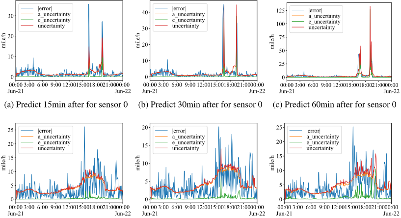
Uncertainty Analysis. In traffic forecasting, most existing methods only provide deterministic traffic predictions without uncertainty. Through the quantitative and visual analysis of uncertainty derived from ST-nFBST, we have uncovered more insights. Figure 2 illustrates the trends of MAE and uncertainties under different prediction horizons. Sensors 0 and 26 represent central and marginal types, respectively. We have the following observations:
- The fluctuation of MAE closely aligns with the variations in uncertainty across diverse forecasting horizons. This implies that our method accurately captures uncertainties. Considering that we thoroughly leverage both uncertainties in the optimization process by incorporating them into
- (d) Predict 15min after for sensor 26 (e) Predict 30min after for sensor 26 (f) Predict 60min after for sensor 26
Figure 2: Comparison between uncertainties and |error| for different forecasting horizons on the METR-LA dataset.
the loss function, this further explains why our approach outperforms other state-of-the-art models.
- In most cases, the aleatoric uncertainty is much larger than the epistemic uncertainty, accounting for the majority of uncertainty. This implies that the traffic uncertainty is mainly data-related. Thanks to the powerful representation capability of neural networks, we can train models effectively to reduce epistemic uncertainty.
- There are some cases where error and uncertainties manifest inconsistently, specifically, with low error but high uncertainties. Moreover, epistemic uncertainty is high in such cases. This occurs when changes in road conditions at intersections, such as traffic congestion or unexpected accidents, result in a sharp decrease in the speed of other sensors. This implies that uncertainty, compared to error, is more effective in monitoring changes in road conditions. A more detailed case study is presented in the Appendix.
- As the forecasting horizon expands, both error and uncertainties of central sensors increase correspondingly, while those of marginal sensors remain relatively stable. However, the predictions of marginal sensors fluctuate significantly at different times. This aligns with the definition of two types of sensors. The marginal sensors exhibit fewer impacts from other sensors while utilizing less information from other sensors. However, the central sensors are more susceptible to the influence exerted by other sensors, rendering predictions more intricate.
4.4 Significance Testing Results
In order to capture the traffic evolution schema, we conduct significance testing from two dimensions: Temporal and Spatial. From Section 2.2, we know that the model's input consists of two parts: a sensor network and a historical sequence composed of observations. Since the sensor network is established once the task is determined (the computation of the weighted adjacency matrix W is calculated before training), our focus is primarily on the testing of Xt.
Testing in the Temporal Dimension. In this experiment, we aim to identify the impact of observations at different times ahead in the input sequence on the prediction. By conducting significance testing on the historical moments of a sensor, we observe that recent historical data (within 30min) generally exhibits significance, yet this may not hold for data over a longer time. Then, we remove different sizes of the historical inputs to reconstruct the input graph signals and retrain using the same network structure. The results are illustrated in Table 2. We have the following observations:
- For short-term forecasting, the historical observations of the past 15 minutes are crucial. The removal of these observations significantly degrades performance and uncertainty, with a worsening effect as the removal window increases. This indicates that short-term forecasting highly depends on historical data of its own.
- For middle-term forecasting, the performance of marginal sensors decreases, while the performance of central sensors remains unchanged or decreases within an acceptable range. This indicates that middle-term forecasting integrates information from both its own and surrounding sensors. When excluding its own historical data, the central sensor can utilize more information from other sensors.
- For long-term forecasting, removing a sensor's historical data demonstrates negligible alterations in performance, even a slight improvement. This indicates that long-term forecasting does not focus on the historical data of itself
| Sensor | Forecasting Horizon | Metric | Initial (-0min) | Reconstruct (-15min) | Reconstruct (-30min) | Reconstruct (-1hour) | Reconstruct (Spatial) |
|---|---|---|---|---|---|---|---|
| 0 (central) | short-term (15min) | MAE | 1.97 | 2.18 | 2.22 | 3.30 5.42 | 1.91 |
| RMSE MAPE | 4.52 | 5.04 | 5.22 | 4.22 | |||
| 5.0% | 5.3% | 5.7% | 5.8% | 4.8% | |||
| Uncertainty | 2.20 | 2.48 | 2.42 | 2.43 | 2.05 | ||
| middle-term (30min) | MAE | 2.46 | 2.42 | 2.52 | 2.47 | 2.17 | |
| RMSE | 6.11 | 5.83 | 6.28 | 6.00 | 5.24 | ||
| MAPE | 6.7% | 6.3% | 6.6% | 6.4% | 5.7% | ||
| Uncertainty | 2.81 | 3.00 | 2.98 | 3.28 | 2.35 | ||
| long-term | MAE | 2.97 | 2.87 | 2.86 | 2.94 | 2.47 | |
| (1hour) | RMSE | 7.51 | 7.02 | 7.17 | 7.39 | 6.13 | |
| MAPE | 8.8% | 8.1% | 8.2% | 7.6% | 6.9% | ||
| Uncertainty | 3.67 | 4.55 | 4.39 | 4.11 | 2.88 | ||
| 181 | MAE | 2.68 | 3.32 | 3.55 | 3.63 | 1.70 | |
| short-term | RMSE | 5.57 | 7.02 | 7.49 | 7.46 | 2.60 | |
| (15min) | MAPE | 6.1% | 8.4% | 9.0% | 9.3% | 2.9% | |
| Uncertainty | 3.00 | 3.52 | 3.81 | 3.58 | 1.68 | ||
| (marginal) | middle-term (30min) | MAE | 3.30 | 3.56 | 3.71 | 3.66 | 1.71 |
| RMSE | 6.85 | 7.59 | 8.08 | 7.50 | 2.84 | ||
| MAPE | 7.7% | 9.1% | 9.7% | 9.2% | 3.0% | ||
| Uncertainty | 3.70 | 3.92 | 4.51 | 4.17 | 1.69 | ||
| long-term | MAE | 3.77 | 3.76 | 3.78 | 3.77 | 1.71 | |
| RMSE | 7.92 | 8.03 | 8.26 | 7.74 | 2.85 | ||
| (1hour) | MAPE | 9.0% | 9.7% | 9.9% | 9.0% | 3.1% | |
| Uncertainty | 4.88 | 4.52 | 5.11 | 4.29 | 1.71 |
but instead utilizes information about the surroundings.
Testing in the Spatial Dimension. In this experiment, we aim to identify the impact of sensors at different locations on the prediction. The testing results indicate that short-term traffic forecasting is more concerned with the road conditions where their sensors are located, but do not pay attention to the situation at intersections. However, the changes at intersections take time to propagate to other road segments and, hence may have a significant impact on long-term forecasting. A more detailed analysis is shown in the Appendix.
Based on the above conclusion, we selectively remove the insignificant sensors to reconstruct the input graph signals and retrain using the same network structure. As illustrated in Table 2, the model's predictive performance and uncertainty significantly improve after retraining on the reconstructed graph signals. Furthermore, due to the rigorous modeling of true relationships and the exclusion of noise that may interfere with the modeling process, the performance is more stable. This validates the efficacy of using significance testing to guide a more deliberate refinement of traffic forecasting.
5 RelatedWork
Traffic forecasting has always been a challenging task due to its complex spatial and temporal dependencies [Wang et al., 2018; Wang et al., 2019b; Ji et al., 2020; Wang et al., 2021; Wang et al., 2023a; Wang et al., 2023b]. Early models in traffic forecasting primarily rely on statistical models [Cressie and Wikle, 2015], such as ARIMA [Ahmed and Cook, 1979; Min and Wynter, 2011] and Bayesian models [Wang et al., 2014]. Recent years have witnessed the emergence of deep learning models to model spatial and temporal dependencies. To extract spatial dependency, some works attempt to use CNN by converting road networks to regular grids [Zhang et al., 2017; Zhang et al., 2019; Ma et al., 2017], while others use GNN and its variants (such as GCN and GAT) by representing road networks as graphs [Jiang and Luo, 2022; Atwood and Towsley, 2016; Kipf and Welling, 2017; Song et al., 2020; Bai et al., 2020; Li et al., 2018; Yu et al., 2018; Li and Zhu, 2021; Wu et al., 2020b; Jiang et al., 2023c; Jiang et al., 2023b; Wu et al., 2020a; Ji et al., 2023]. To extract temporal dependency, some works use RNN and its variants (such as LSTM and GRU) [Ma et al., 2015], while others integrate with convolutional sequence learning or Transformer [Jiang et al., 2023a; Gehring et al., 2017; Ye et al., 2021; Wu et al., 2019; Xu et al., 2020].
In recent years, there has been an increasing focus on exploring the uncertainty in traffic forecasting [Qian et al., 2023; Zhou et al., 2021; Wang et al., 2019a; Liu et al., 2023; Wu et al., 2021]. There are also numerous researches on significance testing for neural networks from parametric [White, 1989b; White, 1989a; Olden and Jackson, 2002] or non-parametric [Lavergne and Vuong, 1996; Lavergne and Vuong, 2000; Fan and Li, 1996; Racine, 1997]. However, testing is limited by the non-identifiability of neural networks or certain assumptions. [Horel and Giesecke, 2020; Liu et al., 2024] have yielded impressive results from Frequentist and Bayesian perspectives respectively. Nevertheless, a notable gap persists in the realm of traffic forecasting.
6 Conclusion
In this paper, we propose to conduct the Full Bayesian Significance Testing for neural networks in Traffic Forecasting, called ST-nFBST. It is a Bayesian framework incorporating spatial-temporal modeling, uncertainty quantification, and significance testing. To the best of our knowledge, we are the first to capture the inherent evolution schema in traffic forecasting through significance testing for neural networks. Moreover, it can effectively detect changes in traffic conditions, identify the inherent traffic schema, and provide guidance for reconstructing the input graph signals.
Acknowledgments
This work was supported by the National Key R&D Program of China (2021ZD0111200). Prof. Wang's work was supported by the National Natural Science Foundation of China (No. 72171013, 72222022, 72242101). Dr. He's work was supported by the China National Postdoctoral Program for Innovative Talents (BX20230195).
@inproceedings{ijcai2024p245,
  title     = {Full Bayesian Significance Testing for Neural Networks in Traffic Forecasting},
  author    = {Liu, Zehua and Wang, Jingyuan and Li, Zimeng and He, Yue},
  booktitle = {Proceedings of the Thirty-Third International Joint Conference on
               Artificial Intelligence, {IJCAI-24}},
  publisher = {International Joint Conferences on Artificial Intelligence Organization},
  editor    = {Kate Larson},
  pages     = {2216--2224},
  year      = {2024},
  month     = {8},
  note      = {Main Track},
  doi       = {10.24963/ijcai.2024/245},
  url       = {https://doi.org/10.24963/ijcai.2024/245},
}
TY - CPAPER TI - Full Bayesian Significance Testing for Neural Networks in Traffic Forecasting AU - Liu, Zehua AU - Wang, Jingyuan AU - Li, Zimeng AU - He, Yue T2 - Proceedings of the Thirty-Third International Joint Conference on Artificial Intelligence, IJCAI-24 PB - International Joint Conferences on Artificial Intelligence Organization PY - 2024 SP - 2216 EP - 2224 DO - 10.24963/ijcai.2024/245 UR - https://doi.org/10.24963/ijcai.2024/245 ER -Copied
Machine-readable versions of this paper, for tools and AI agents:





