
SaSDim:Self-Adaptive Noise Scaling Diffusion Model for Spatial Time Series Imputation
Proceedings of the Thirty-Third International Joint Conference on Artificial Intelligence. Main Track. Pages 2561-2569.
https://doi.org/10.24963/ijcai.2024/283
Keywords
- Data Mining: DM: Mining spatial and/or temporal data
Abstract
Spatial time series imputation is of great importance to various real-world applications. As the state-of-the-art generative models, diffusion models (e.g. CSDI) have outperformed statistical and autoregressive based models in time series imputation. However, diffusion models may introduce unstable noise owing to the inherent uncertainty in sampling, leading to the generated noise deviating from the intended Gaussian distribution. Consequently, the imputed data may deviate from the real data. To this end, we propose a Self-adaptive noise Scaling Diffusion Model named SaSDim for spatial time series imputation. Specifically, we introduce a novel Probabilistic High-Order SDE Solver Module to scale the noise following the standard Gaussian distribution. The noise scaling operation helps the noise prediction module of the diffusion model to more accurately estimate the variance of noise. To effectively learn the spatial and temporal features, a Spatial guided Global Convolution Module (SgGConv) for multi-periodic temporal dependencies learning with the Fast Fourier Transformation and dynamic spatial dependencies learning with dynamic graph convolution is also proposed. Extensive experiments conducted on three real-world spatial time series datasets verify the effectiveness of SaSDim.
- [Alcaraz and Strodthoff, 2022] Juan Miguel Lopez Alcaraz and Nils Strodthoff. Diffusion-based time series impu- tation and forecasting with structured state space models. arXiv preprint arXiv:2208.09399, 2022.
- [Cao et al., 2018] Wei Cao, Dong Wang, Jian Li, Hao Zhou, Lei Li, and Yitan Li. Brits: Bidirectional recurrent im- putation for time series. Advances in neural information processing systems, 31, 2018.
- [Che et al., 2018] Zhengping Che, Sanjay Purushotham, Kyunghyun Cho, David Sontag, and Yan Liu. Recurrent neural networks for multivariate time series with missing values. Scientific reports, 8(1):6085, 2018.
- [Cini et al., 2022] Andrea Cini, Ivan Marisca, and Cesare Alippi. Filling the g ap s: Multivariate time series im- putation by graph neural networks. In ICLR, 2022.
- [Du et al., 2023] Wenjie Du, David Côté, and Yan Liu. Saits: Self-attention-based imputation for time series. Expert Systems with Applications, 219:119619, 2023.
- [Goel et al., 2022] Karan Goel, Albert Gu, Chris Donahue, and Christopher Ré. It's raw! audio generation with state- space models. In Proceedings of International Conference on Machine Learning, pages 7616-7633. PMLR, 2022.
- [Gu et al., 2021] Albert Gu, Karan Goel, and Christopher Ré. Efficiently modeling long sequences with structured state spaces. arXiv preprint arXiv:2111.00396, 2021.
- [Hewage et al., 2020] Pradeep Hewage, Ardhendu Behera, Marcello Trovati, Ella Pereira, Morteza Ghahremani, Francesco Palmieri, and Yonghuai Liu. Temporal con- volutional neural (tcn) network for an effective weather forecasting using time-series data from the local weather station. Soft Computing, 24:16453-16482, 2020.
- [Li et al., 2022] Yuhong Li, Tianle Cai, Yi Zhang, Deming Chen, and Debadeepta Dey. What makes convolutional models great on long sequence modeling? arXiv preprint arXiv:2210.09298, 2022.
- [Lim and Zohren, 2021] Bryan Lim and Stefan Zohren. Time-series forecasting with deep learning: a sur- vey. Philosophical Transactions of the Royal Society A, 379(2194):20200209, 2021.
- [Luo et al., 2018] Yonghong Luo, Xiangrui Cai, Ying Zhang, Jun Xu, et al. Multivariate time series imputation with generative adversarial networks. Advances in neural information processing systems, 31, 2018.
- [Marisca et al., 2022] Ivan Marisca, Andrea Cini, and Ce- sare Alippi. Learning to reconstruct missing data from spa- tiotemporal graphs with sparse observations. Advances in Neural Information Processing Systems, 35:32069-32082, 2022.
- [Nelson, 1998] Brian K Nelson. Time series analysis using autoregressive integrated moving average (arima) models. Academic emergency medicine, 5(7):739-744, 1998.
- [Nguyen et al., 2022] Eric Nguyen, Karan Goel, Albert Gu, Gordon Downs, Preey Shah, Tri Dao, Stephen Baccus, and Christopher Ré. S4nd: Modeling images and videos as multidimensional signals with state spaces. Advances in neural information processing systems, 35:2846-2861, 2022.
- [Song et al., 2020] Yang Song, Jascha Sohl-Dickstein, Diederik P Kingma, Abhishek Kumar, Stefano Ermon, and Ben Poole. Score-based generative modeling through stochastic differential equations. arXiv preprint arXiv:2011.13456, 2020.
- [Tashiro et al., 2021] Yusuke Tashiro, Jiaming Song, Yang Song, and Stefano Ermon. Csdi: Conditional score- based diffusion models for probabilistic time series impu- tation. Advances in Neural Information Processing Sys- tems, 34:24804-24816, 2021.
- [Wang et al., 2020] Senzhang Wang, Jiannong Cao, and S Yu Philip. Deep learning for spatio-temporal data min- ing: A survey. IEEE transactions on knowledge and data engineering, 34(8):3681-3700, 2020.
- [Wang et al., 2021] Qinfen Wang, Siyuan Ren, Yong Xia, and Longbing Cao. Bicmts: Bidirectional coupled mul- tivariate learning of irregular time series with missing val- ues. In Proceedings of the 30th ACM International Con- ference on Information & Knowledge Management, pages 3493-3497, 2021.
- [Wang et al., 2022a] Senzhang Wang, Jiyue Li, Hao Miao, Junbo Zhang, Junxing Zhu, and Jianxin Wang. Generative- free urban flow imputation. In Proceedings of the 31st ACM International Conference on Information & Knowl- edge Management, pages 2028-2037, 2022.
- [Wang et al., 2022b] Senzhang Wang, Jiyue Li, Hao Miao, Junbo Zhang, Junxing Zhu, and Jianxin Wang. Generative- free urban flow imputation. In Proceedings of the 31st ACM International Conference on Information & Knowl- edge Management, pages 2028-2037, 2022.
- [Wu et al., 2022] Haixu Wu, Tengge Hu, Yong Liu, Hang Zhou, Jianmin Wang, and Mingsheng Long. Timesnet: Temporal 2d-variation modeling for general time series analysis. In The Eleventh International Conference on Learning Representations, 2022.
- [Xu et al., 2022] Xin Xu, Liangliang Zhang, Qi Kong, Chen- guang Gui, and Xing Zhang. Enhanced-historical aver- age for long-term prediction. In 2022 2nd International Conference on Computer, Control and Robotics (ICCCR), pages 115-119. IEEE, 2022.
- [Yang et al., 2022] Ling Yang, Zhilong Zhang, Yang Song, Shenda Hong, Runsheng Xu, Yue Zhao, Yingxia Shao, Wentao Zhang, Bin Cui, and Ming-Hsuan Yang. Diffusion models: A comprehensive survey of methods and applica- tions. arXiv preprint arXiv:2209.00796, 2022.
- [Yi et al., 2016] Xiuwen Yi, Yu Zheng, Junbo Zhang, and Tianrui Li. St-mvl: filling missing values in geo-sensory time series data. In Proceedings of the 25th International Joint Conference on Artificial Intelligence, 2016. IJCAI
- [Yoon et al., 2017] Jinsung Yoon, William R Zame, and Mi- haela van der Schaar. Multi-directional recurrent neural networks: A novel method for estimating missing data. In Proceedings of Time series workshop in international con- ference on machine learning, 2017.
- [Yoon et al., 2018] Jinsung Yoon, James Jordon, and Mi- haela Schaar. Gain: Missing data imputation using genera- tive adversarial nets. In Proceedings of International con- ference on machine learning, pages 5689-5698. PMLR, 2018.
- [Yu et al., 2016] Hsiang-Fu Yu, Nikhil Rao, and Inderjit S Dhillon. Temporal regularized matrix factorization for high-dimensional time series prediction. Advances in neu- ral information processing systems, 29, 2016.
References were extracted automatically from the PDF and may contain errors.
Full text extracted automatically from the PDF; figures, tables and equations may differ. The PDF is the version of record.
1 Introduction
Spatial time series is a type of data that describes the time series relationship within and between locations distributed across space, such as the traffic flow data collected from a set of road sensors deployed in a road network [Wang et al., 2020]. To collect the observations of spatial time series, generally, a significant number of sensors, such as cameras and traffic sensors, are needed to be deployed. However, a complete spatial time series is usually unavailable due to various factors, including sensor malfunctions, unstable communication signals, non-uniform sensor distribution, and the stochastic and dynamic nature of data, leading to data anomalies or missing [Lim and Zohren, 2021]. Therefore, how to impute the incomplete spatial time series data is a primary challenge that needs to be addressed before further data analysis.
Traditionally, statistical methods such as ARIAM [Nelson, 1998] and HR [Xu et al., 2022] are adopted for modeling time series. To further capture the spatial correlations of the time series data collected from different locations, matrix completion, and tensor decomposition approaches are utilized [Yu et al., 2016]. However, it is difficult for these statistical based methods to capture the complex spatiotemporal relationships. Recently, deep learning methods such as CNN, RNN, and transformer have also been widely adopted for spatiotemporal data imputation. The RNN-based models, such as BRITS [Cao et al., 2018] and ASTCMCN [Wang et al., 2022a], impute missing values in an autoregressive way. However, biases can accumulate within the recursive structure of RNNs, ultimately impacting the model accuracy. CNN-based models try to capture the temporal correlations of the time series with convolutional kernels. However, the limited receptive field of CNN makes it difficult to capture global temporal correlations [Hewage et al., 2020]. To address this issue, transformer-based models such as SAITS [Du et al., 2023] and SPIN [Marisca et al., 2022] apply attention mechanism to capture the global temporal dependencies. To model the multi-periodicity in time series, State Space Models (SSM) uses Fast Fourier Transform (FFT) to project time series from the time domain to the spectral domain, and aggregates features with different frequencies in the spectral domain [Gu et al., 2021; Nguyen et al., 2022]. However, SSM cannot effectively learn the spatial features of spatial time series.
Recently, diffusion models have been applied for spatial time series imputation and achieved better performance than autoregressive based methods. As the first diffusion modelbased method, CSDI [Tashiro et al., 2021] utilizes scorebased diffusion conditioned on observed data for time series imputation. SSSD [Alcaraz and Strodthoff, 2022] further combines diffusion models and structured state space models to more effectively capture the long-term temporal dependencies in time series data. Generally, diffusion models create a forward process that learns a map from the ground truth to noise and a backward process to reconstruct data from noise to ground truth. Specifically, the forward process in diffusion models introduces the Gaussian noise into the data step by step. However, due to the uncertainty of sampling, the distribution of sampled noise may not really follow the Gaussian distribution. This inconsistency may lead to bias, thus ultimately causing the imputed data to deviate from the real data. Another issue of current diffusion models is that they are less effective to capture the complex spatial and temporal features of the spatial time series data. For example, the multi-periodic temporal dependencies in time series are hard to be learned by CSDI and SSSD models.
To address the above issues, we propose a Self-adaptive Noise Scaling Diffusion Model named SaSDim. SaSDim can adaptively scale the sampled noise in the forward process to make the distribution of the noise more stable, and effectively capture the multi-periodicity temporal dependencies and dynamic spatial dependencies. Specifically, SaSDim contains three major modules, the Conditional Mixture Module, the Spatial guided Global Convolution (SgGConv) module, and the Probabilistic High-Order Stochastic Differential Equation (SDE) Solver Module. The Conditional Mixture Module encodes the spatial time series data and extracts the multiperiodicity temporal features with FFT. Inspired by SGConv [Li et al., 2022], SgGConv explicitly models the temporal dependencies with different time scales and captures the dynamic spatial dependencies. To be specific, SgGConv first decomposes a time series into components with different frequencies in the spectral domain. Then SgGConv measures the importance of each component by linearly combining each frequency and projects these frequencies back to the time domain to explicitly model the multi-periodic time series. The frequencies are further combined with the spatial convolution, which reflects spatial correlations among the time series generated from different locations. Finally, we use the Probabilistic High-Order SDE Solver Module to scale the noise at each time step by generating and optimizing the learnable coefficient of high-order SDEs. The primary contributions of this work are summarized as follows.
- We for the first time introduce a noise scaling mechanism in diffusion model to address the data generation bias issue caused by unstable noise sampling in forward process for more accurate spatial time series imputation.
- We propose the Spatial guided Global Convolution module named SgGConv to effectively capture the complex spatial correlations as well as the multi-periodic temporal dependencies simultaneously.
- Extensively evaluations on three real-world datasets demonstrate that the proposed Probabilistic High-Order SDE Solver Module can effectively enhance the noise stability of the conventional diffusion models, and the SgGConv module can effectively capture the spatiotemporal correlations.
2 RelatedWork
Traditionally, statistical methods were used for time series imputation, such as K-Nearest Neighbors (KNN), Matrix Factorization (MF) [Yu et al., 2016] and Multiple Imputation using Chained Equations. With the great success of deep learning models in spatial and temporal feature learning, RNN-based deep learning methods were also adopted. Deep autoregressive models based on recurrent neural networks
(RNNs) are among the most popular approaches [Che et al., 2018; Wang et al., 2021; Yoon et al., 2017]. BRITS [Cao et al., 2018] is a representative model that utilizes bidirectional RNNs for spatial time series imputation and uses a linear regression layer to incorporate spatial information. Modeling the global temporal dependency is challenging for RNN models. To address this issue, SAITS introduced self-attention to capture the global temporal features [Du et al., 2023]. SPIN further adopted joint attention that combined spatial and temporal attention to model information exchange between different time series [Marisca et al., 2022]. ASTCMCN effectively combined transformer with RNN to capture both temporal and spatial dependencies for spatiotemporal data imputation [Wang et al., 2022b].
Motivated by the great success of generative models, recent works tried to impute missing data using generativebased models. GAIN proposed to use generative adversarial networks (GANs) for data imputation [Yoon et al., 2018]. GAINFilling tried to generate sequences by matching the underlying data distribution [Luo et al., 2018]. CSDI proposed to apply Denoising Diffusion Probabilistic Models (DDPM) for data imputation [Tashiro et al., 2021]. It sequentially employed feature and temporal attention to learn the noise at each step, while introducing conditions in the denoising process. However, these methods suffer from the issue of parameter explosion as the increase of the length of the time series, making researchers search for lightweight and more efficient feature extractors for time series modeling.
Recently, State Space Models (SSM) [?; Nguyen et al., 2022; Goel et al., 2022] have shown promising results in sequence modeling. SSM used a set of linear dynamics equations to model nonlinear and physical systems with input, output, and state variables. However, these models lack heuristics due to their long mathematical proof. Inspired by these methods, [Li et al., 2022] proposed SGConv, which generated global convolution kernels by upsampling local convolution kernels before concatenating them. SGConv effectively modeled the distance-dependent decays among nodes in a sequence and kept the parameter scale sublinear with respect to the sequence length. While achieving promising results, SGConv cannot well catch the spatial information among graph nodes. This leads to limited performance improvement in time series imputation. More recently, a Fourier Transformbased deep method called TimesNet [Wu et al., 2022] was proposed. It adapted the spectral characteristics of spatial time series to capture correlations within and across periods through multi-scale convolutions. However, limited by the convolutional kernel, TimesNet cannot effectively capture the spatial correlations and the multi-periodic temporal dependencies simultaneously.
3 Preliminary and ProblemDefinition
In this section, we will first define some terminologies, and then give a formal problem definition.
Definition 1. Spatial graph Given the spatial distribution of the sensors (e.g. traffic sensors) for time series data collection, we construct a spatial graph G = (V,E) based on the spatial distance between each pair of sensors, where V = {v1, ..., vN} is a set of sensor nodes deployed in the space and E is the edge set connecting the sensor nodes.
| Notations | Descriptions |
|---|---|
| X | Spatial time series data |
| N | The number of the spatial nodes |
| βt, αt, ˆαt | Constant hyperparameters of diffusion model |
| ϵθ | Noise prediction model |
| F | Fast Fourier Transform |
| K | Convolutional kernel |
| G | Spatial graph |
| ∆t | The cost of time from a time step to its neighbor step |
| ∇ | The first order derivative operator |
| r | The high order coefficient of SDE |
Definition 2. Spatial Time Series. We denote X ∈ RN×D as the time series observations on spatial graph G. We denote the incomplete and complete spatial time series at time t as Xt ∈ RN×D and Zt ∈ RN×D , respectively, where N is the number of spatial nodes (e.g. traffic sensors deployed at different locations) and D is the length of the time series.
The historical spatial time series can be represented as a sequence X = (Xt-k, ...,Xt). To conduct the spatial time series imputation over the locations where the data are unavailable, we also define the mask matrix of incomplete data as follows,
where vn denotes the n-th sensor node and t is the time. Mt(vn) is a data mask matrix. We mark the element without observations as 0 and the element with data as 1.
To use the FFT, we need to introduce the convolution theorem first, which is a communication theory as follows,
where ∗ is a convolution operation, · is a multiply operation. F represents FFT, which can be used to convolve time series. For time series X, it can be convolved by convolution kernel K by using FFT, which is similar to a time convolution operation.
Problem Definition 1. Given the spatial graph G = (V, E) and the corresponding incomplete spatial time series X = (X0, . . . ,XT ), we aim to build a model ϵθ to impute X and obtain a complete spatial time series Z = (Z0, . . . , ZT ).
4 Methodology
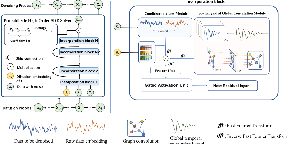
The model framework of SaSDim is shown in Figure 1, which contains the Conditional Mixture Module (CMM), the Spatial guided Global Convolution (SgGConv) module, and the Probabilistic High-Order SDE Solver Module (SDEM). CMM provides conditions to accelerate the convergence of SgGConv. SDEM aims to adaptively scale the predicted noise in the forward process. In summary, SaSDiM is a score-based conditional diffusion model. SgGConv and CMM integrate as the denoising score function, while SDEM outputs a highorder coefficient of the map from noisy data to the ground truth. Next, we will introduce the model in detail.
4.1 Conditional Mixture Module
In this module, we use a Conv1D encoder to embed the sequence relation and spatial information to guide the generation of a diffusion model. Specifically, the input data Xt in Figure 1 which contains noise during the denoising process, is first concatenated with a spatial time series data embedding that incorporates local information, which serves as a guidance for generation. Next, following the convolution theorem presented in the preliminary, the concatenated tensor is computed to extract the frequency feature through FFT. Then it is multiplied with convolution kernels from the SRGConv module and calculated from frequency feather to series. Additionally, diffusion embedding, feature embedding, and time step embedding are included as supplementary information and added to the tensor after this operation.
Then, the tensor goes through a layer of gated activation units before entering the next layer of residual units. The results of several residual layers are added to the output, which maintains its original state through skip connections, and then they are fed into the probabilistic high-order SDE solver. Briefly, we learn a function f in each residual layer. f transforms the input XL-1 to the output XL.
where L is the number of layers.
4.2 Spatial Guided Global ConvolutionModule
FFT is an effective tool to extract frequency features. In numerical computing, it is known as Discrete Fourier Transform (DFT) or FFT algorithm. DFT simplifies the numerous frequencies in a sequence to a smaller set of time series length L components. This helps us calculate their weighted sum, similar to the convolution operation.
Based on this idea and inspired by SGConv, we propose the spatial-guided Global Convolution. Convolutional kernels gather information from nearby neighbors in a sequence, following the "closer means stronger" rule [Li et al., 2022]. For example, spatial graph convolution groups locations based on distances, and SGConv uses wave attenuation for temporal kernels. We further combine temporal kernels using graph spectrum information to build the spatial-guided global convolutional kernels. These represent a weighted sum of frequency components underlining each node, which can explicitly model the temporal correlations and dynamics.
Following this idea, we propose SRGConv which includes the Global Temporal Convolution and Dynamic Graph Convolution. First, the Global Temporal Convolution for modeling temporal correlation generates convolutional kernels Ki that build upon the wave curves with decay. Then we sum all the kernels as follows,
convolution kernel
Figure 1: The model framework of SaSDim. The right side of the figure shows the details of the Conditional Mixture Module and the Spatial guided Global Convolution Module. The left side of the figure is the Probabilistic High-Order SDE Solver Module. The bottom is the explanation of symbols.
where Nk is the number of kernels. These kernels gather information from nearby elements in a time series. Following the DFT algorithm, it convolves temporal information by a weighted sum of the frequencies.
We next introduce the Dynamic Graph Convolution for modeling the spatial correlations. We have
where Wλ is a scaling factor and f is the injection function which can be written as
where (α0, . . . , αN) is the scaling factor corresponding to each node. The transformation F modifies the adjacent matrix among them with scaling factor so that we can inject it to the same size as time dimensions via injection function f. It is a dimensionality reduction so that the adjacent matrix can linearly combine the elements of the temporal kernel in the time dimension.
Finally, we combine the Global Temporal Convolution and Dynamic Graph Convolution by element-wise multiplication to obtain the Spatial guided Global Convolution. This combined operation φ ¯ A(K) integrates the strengths of both convolutions, allowing for more comprehensive dynamic temporal information extraction, which can be written as
where ¯ A is calculated by P ¯ λAP T , P is a positive definite matrix and P T is the transpose matrix of P with ¯ λA representing the eigenvalue matrix of A. According to the Convolution Theorem and Eq(6), the theorem equation can be rewritten as
Based on this formula, we compute a mapping from the time field to the spectral field and multiply them. Then we map the result back to the time field. During the process, frequency components are weighted and summed across nodes, where the kernel is regarded as the weight. Finally, we send the output from SgGConv to the Feature unit as shown in Figure 1, which can be considered as an attention to capture the spatial correlations.
4.3 Probabilistic High-Order SDE Solver
We first introduce the traditional stochastic differential equations (SDEs) that present the forward process. Then, we present our method that finds a new training loss to scale the unstable noise to a proper level. To be consistent with the representation of stochastic differential equations, X is denoted as x in the following sections.
First, SDEs perturb data to noise with a diffusion process governed by the following stochastic differential equation (SDE) [Yang et al., 2022]
where f(x, t) and g(t) are diffusion and drift functions of the SDE, and w is a standard Wiener process. The forward process of denoising diffusion probabilistic model (DDPM)
discretizes the SDE so that it can be considered as the limit of the following discrete form as ∆t → 0:
For the sampling process, given t′ = t+∆t, its discrete form can be written as follows,
Continualizing this form, we can get
To achieve better results, we have computed the reverse process that includes higher-order derivatives.
Fact: The training loss function can be represented as:
To prove that, we need two lemmas as follows,
Lemma 1. High-order stochastic differential equation of equation (4) can be represented as
when ∆t → 0 and ψ(∇x) = f (x, t) - g(t)2∇x log qt(x). βx is an upper bound of ∆x.
Lemma 2. Given the traditional sampling equations
we can get sampling equations of lemma1
For more details of the two lemmas, one can refer to the Appendix.
By using stochastic differential equations to present the forward and backward process, we can calculate the score function ∆xt log p(xt|x0) (which can also be written as ϵθ or sθ) which is equivalent to approximate ϵ. This is also called score matching [Song et al., 2020]. Thus the coefficient of the score function can be written in Algorithm 1, line 7.
Regarding the range of r according to lemma2, we adopt a probabilistic sampling approach by sampling several points from a Gaussian distribution. Among these points, one is selected as the initial value for r. Considering that the magnitude of higher-order derivatives is smaller than that of the first-order derivative, the values of r are confined within a window on the Gaussian distribution.
During the training process, the noise predictor ϵθ is optimized to predict the noise each step with the help of the high order score function. Then we gain a high order coefficient r after each epoch optimizition. While selecting t in uniform distribution (Algorithm 1, line 3), its mathematical expectation is the average of all r. The mathematical expectation is varied according to the unstable noise. As a result, it scales down the intensity.
Algorithm 1 Training of SaSDiM
- 1: Input: Distribution of training data q(x0), the number of iteration N, the sequence of noise levels {αt}, high order coefficient r initialized as a variant;
- 2: Output: Trained denoising function ϵθ and a list of coefficient R;
- 3: for i = 1 to N do
- 4: t ∼ Uniform({1, . . . , T}), x0 ∼ q(x0), R initialized as a list;
- 5: ϵ ∼N(0, I);
- 6: Calculate noisy xt = ¯αtx0 + ¯ βtϵ;
- 7: Take gradient step on ∇θ||(ϵ - (1 + r)ϵθ)||22 , where ϵθ = ϵθ(xt, t | ˆ x0);
- 8: R[i] = r;
- 9: end for
Algorithm 2 Imputation (Sampling) with SaSDiM
- 1: Input: Trained denoising function ϵθ, high order coefficient list R;
- 2: Output: Imputed missing values x0;
- 3: r = ∑Ni=1 Ri ∗ (1/N);
- 4: xT ∼ N(0, I), where the dimension of xT corresponds to the missing indices of ˆ x0;
- 5: for t = T to 1 do
- 6: Sample xt-1 by using the sampling equations presented in lemma2;
- 7: end for
4.4 Implementation Details
The initialization of coefficient r of high-order SDE is in the range from 0 to 0.2. We set the maximum noise level to 0.02 and the layer of block to 4. The model is implemented using Pytorch and trained in an end-to-end manner using Adam with a learning rate of 0.001. We introduce the setting details in Table ??.
5 Experiment
5.1 Datasets
We evaluate the performance of our model on three spatial time series datasets, METR-LA, AQI-36, and PEMS-BAY. METR-LA is a dataset used in traffic flow prediction and imputation. It contains 207 traffic sensor nodes in Los Angeles County Highway with a minute-level sampling rate. AQI36 is collected from 36 AQI sensors distributed across the city of Beijing. This dataset serves as a widely recognized benchmark for imputation techniques and includes a mask used for evaluation that simulates the distribution of actual missing data [Yi et al., 2016]. For a specific month, such as January, this mask replicates the patterns of missing values from the preceding month. Across all scenarios, the valid observations that have been masked out are employed as targets for evaluation. PEMS-BAY is an open dataset used for traffic flow prediction and analysis, primarily covering the transportation network of the Bay Area in California, USA. The dataset comprises 325 sensor nodes with a sampling interval of 5 minutes, and it contains a total of 16,937,700 data points.
| Description | AQI-36 | METR-LA | PEMS-BAY |
|---|---|---|---|
| Batch size | 16 | 16 | 16 |
| Time length L | 24 | 24 | 24 |
| Epochs | 200 | 200 | 200 |
| Learning rate | 0.001 | 0.001 | 0.001 |
| Channel size d | 64 | 64 | 64 |
| Minimum noise level β1 | 0.0001 | 0.0001 | 0.0001 |
| Maximum noise level βT | 0.5 | 0.2 | 0.2 |
| Diffusion steps T | 50 | 50 | 50 |
In total, each dataset will be artificially masked 25% or 50% values at random. For the two datasets METR-LA and PEMSBAY, we partition the entire data into training, validation, and testing sets by a ratio of 8 : 1: 1. We evaluate our model performance under two metrics Mean Absolute Error (MAE) and Root Mean Square Error (RMSE).
5.2 Baselines
We compare our model with the following baselines.
- Transformer calculates the average value of nearby nodes based on geographic distance to impute.
- SAITS [Du et al., 2023] is a method based on diagonally-masked self-attention (DMSA) and joint optimization.
- BRITS [Cao et al., 2018] utilizes bidirectional RNN and MLP to integrate spatiotemporal features.
- TimesNet [Wu et al., 2022] is a self-organized convolution model for time series imputation.
- SPIN [Marisca et al., 2022] employs threshold graph attention and temporal attention jointly to implicitly model spatiotemporal sequences.
- GRIN [Cini et al., 2022] is a bidirectional GRU-based method with graph neural network for multivariate time series imputation.
- CSDI [Tashiro et al., 2021] is a probability imputation method based on the conditional diffusion probability model, which treats different nodes as multiple features of the time series, and uses a Transformer to capture the feature dependencies.
5.3 Experiment Result
The result shown in Table 3 indicates that BRITS performs not well among all the baseline models because the MLP model cannot effectively capture the spatial correlations and the higher-order relationships between nodes without a good spatial encoding. SAITS shows slightly better performance, indicating that Diagonally-Masked Self-Attention can alleviate the impact of self-redundant information and improve temporal prediction performance. SPIN outperforms other baseline models, suggesting that the improved attention mechanism with Hybrid Spatiotemporal Attention is effective in enhancing the performance of the original Transformer for spatial time series. The result of TimesNet results is slightly lower than those of SPIN from 1% to 10%, suggesting that while models that adaptively organize data for temporal convolution can effectively capture the temporal correlations, this convolution approach limits the ability to learn the global spatiotemporal dependencies. SaSDim achieves the best results in terms of two metrics in most cases with only three exceptions that achieve the second best results. Specifically, with a missing rate of 50% on the AQI-36 dataset, the MAE of SaSDim drops by 11% compared to SPIN. This confirms that the SgGConv module can better model the dynamic global temporal interaction. SaSDim achieves performance improvement by 7.5% compared to CSDI. One can also see that CSDI performs as well as SaSDim on the AQI-36 dataset but is surpassed by SaSDim by 20% on the METR-LA dataset. This demonstrates the superiority of SaSDim in modeling spatial time series compared with existing diffusion model-based approaches.
To further evaluate the performance of different methods under very high point data missing percentages, we compare SaSDiM against the baselines when p% = 75% and p% = 95%. The result is shown in Table 4. It demonstrates again that SaSDiM outperforms all the baselines when the available time series observations are very sparse.
5.4 Ablation Study
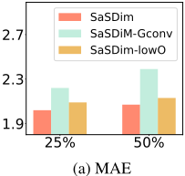
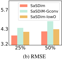
To study whether each module of SaSDim is useful to the studied problem, we also compare SaSDim with two variants for ablation study. SaSDim-lowO is a variant of SaSDim that removes the probabilistic high-order SDE-solver module. SaSDim-GConv only captures the temporal global relations without using spatial guidance.
Figure 3 shows the RMSE and MAE bars for the two variants compared to SaSDim. It shows that SaSDim-GConv performs significantly worse than the other variants by 25% on 25% data missing scenario because it does not consider the geographical correlations between locations. The Constraint module is used to modulate the adjacency relationships between nodes.
SaSDim-lowO directly applies first-order derivatives in the denoising process. Although SaSDim-lowO is superior to other variants, it still performs worse than SaSDim, significantly lagging behind SaSDim with a 15% higher RMSE and
| Model | AQI-36 | PEMS-BAY | METR-LA | |||||||||
|---|---|---|---|---|---|---|---|---|---|---|---|---|
| 25% | 50% | 25% | 50% | 25% | 50% | |||||||
| RMSE | MAE | RMSE | MAE | RMSE | MAE | RMSE | MAE | RMSE | MAE | RMSE | MAE | |
| Transformer | 29.46 | 16.26 | 31.49 | 17.45 | 2.98 | 1.63 | 3.22 | 1.74 | 7.01 | 2.82 | 7.16 | 2.89 |
| BRITS | 28.76 | 15.72 | 29.12 | 16.01 | 2.85 | 1.59 | 3.02 | 1.67 | 6.93 | 2.80 | 7.13 | 2.85 |
| SAITS | 29.85 | 16.24 | 30.97 | 17.18 | 2.34 | 1.35 | 2.57 | 1.42 | 6.23 | 2.66 | 6.51 | 2.73 |
| CSDI | 14.52 | 7.71 | 16.93 | 8.87 | 1.49 | 0.76 | 1.77 | 0.85 | 4.05 | 2.27 | 4.38 | 2.32 |
| TimesNet | 15.01 | 12.38 | 17.49 | 13.22 | 1.88 | 0.92 | 2.14 | 0.97 | 5.33 | 2.49 | 5.76 | 2.55 |
| GRIN | 12.93 | 7.93 | 15.81 | 9.02 | 1.70 | 0.85 | 1.92 | 0.91 | 4.21 | 2.30 | 4.47 | 2.35 |
| SPIN | 12.98 | 7.56 | 16.53 | 9.11 | 1.62 | 0.81 | 1.83 | 0.86 | 4.25 | 2.32 | 4.51 | 2.39 |
| SaSDiM | 12.21 | 7.03 | 14.33 | 8.22 | 1.30 | 0.69 | 1.48 | 0.76 | 3.81 | 2.02 | 4.11 | 2.07 |
| Model | METR-LA | PEMS-BAY | ||
|---|---|---|---|---|
| 75 % | 95 % | 75 % | 95 % | |
| BRITS | 3.02 | 5.19 | 2.17 | 3.91 |
| SAITS | 3.74 | 6.72 | 2.96 | 7.40 |
| Transformer | 2.71 | 5.13 | 1.13 | 2.70 |
| GRIN | 2.39 | 4.08 | 1.09 | 2.70 |
| SPIN | 2.24 | 2.89 | 1.09 | 2.26 |
| SaSDiM | 2.18 | 2.93 | 1.05 | 2.20 |
20% higher MAE in the 25% data missing scenario. This indicates that SaSDim can learn better representations by scaling down the noise for denoising.
5.5 Parameter Study
To analyze the parameter used in SaSDim, the scaling factor of the graph is initialized using a standard normal distribution. When the maximum value in the scaling factor array is larger than one, the values in the scaling factor array that are relatively smaller than the maximum value will become larger. Since the scaling factor array still follows a normal distribution, the difference between the maximum and minimum values will increase under equal probability. This led to an increase in the variance of the convolutional kernels and an increase in uncertainty. When the minimum value in the scaling factor array is smaller than zero, it greatly increases the uncertainty of the graph. For an extreme example, when all the coefficients in the scaling factor array are negative, the adjacency matrix becomes a negative matrix, causing the matrix to lose its physical meaning.
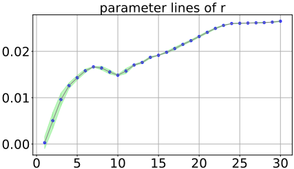
Finally, we study the effect of coefficients r of the probabilistic high-order SDE solver on the mode performance. According to the equation in the Appendix, the absolute value of r should be smaller than one, so we initially set the values of r to a value in the range between -1 and 1. To better observe the trajectory and trend of r during training, we set the initial value of r to zero. The results show that r gradually increases after a sudden decrease and eventually stabilizes around 0.026 as shown in Figure 3. This indicates that the noise scales down step by step. Next, to determine the final shared value of r for sampling, we conduct two experiments. In one experiment, we set r to be the last value obtained during optimization, and in the other experiment, we take the average of all the optimized r values. The results show that setting r to the last value obtained leads to significant fluctuations in performance while using the average value yields stable results. This suggests that taking the average value mitigates the impact of randomness.
6 Conclusion
This paper proposes a method called SaSDim inspired by global convolution and Denoising Diffusion Probabilistic Model learning framework for spatial time series imputation. SaSDim employs SgGConv to capture the global dynamic interactions among time steps. SgGConv models the temporal correlations with spatial information by generating dynamic temporal convolution kernels with spatial guidance. SaSDim optimizes the coefficients r of the high-order SDE solver during the training process to facilitate the generation of shared coefficients that scale unstable noise. Experimental results conducted on three real datasets verify the effectiveness of SaSDim.
A Provement
Lemma 1. High-order stochastic differential equation of equation(4) can be represented as
when ∆t → 0 and ψ(∇x) = f(x, t) - g(t)2∇x log qt(x). And βx is an upper bound of ∆x.
Proof. Initially, the discretized form of a high-order stochastic equation can be written as
To go further, let's consider the third-order item as
For the terms involving third-order derivatives, we have ∆x raised to a higher power, and ∆x is proportional to √t. Therefore, as ∆t approaches zero, the third-order terms become higher-order infinitesimals with respect to ∆t. By scaling, we can obtain
where βx is the upper bound of ∆x.
Based on lemma1, we prove
Lemma 2. Given the traditional sampling equations
we can get sampling equations of lemma1
Proof. Given that q(xt|x0) = N(xt; ¯ αtx0, ¯ βt 2 I), where ¯ βt is the total noise intensity coefficient and we can get the equation below:
Then the higher-order derivatives can be represented as
as ∆xt ∼ O(∆(√t)), α is limited to a finite real number. According to lemma1:
and we get ∇xt log q(xt) by
then we get the result only by computing q(xt|x0). Also, in the similar way we can compute ∇xxt log q(xt) with the rule of differentiation of fractions and the equation (8). Then we get it as
To go further, we have
Finally, given sθ(xt, t) = ϵθ, then the training loss can be presented as follows
Given t′ = t +∆t, then the sampling process can be written
Acknowledgements
This research was funded by the National Science Foundation of China (No.62172443), the Science and Technology Major Project of Changsha (No.kh2402004) and Hunan Provincial Natural Science Foundation of China (No.2022JJ30053). This work was carried out in part using computing resources at the High-Performance Computing Center of Central South University.
Contribution Statement
Senzhang Wang is the corresponding author.
@inproceedings{ijcai2024p283,
  title     = {SaSDim:Self-Adaptive Noise Scaling Diffusion Model for Spatial Time Series Imputation},
  author    = {Zhang, Shunyang and Wang, Senzhang and Tan, Xianzhen and Wang, Renzhi and Liu, Ruochen and Zhang, Jian and Wang, Jianxin},
  booktitle = {Proceedings of the Thirty-Third International Joint Conference on
               Artificial Intelligence, {IJCAI-24}},
  publisher = {International Joint Conferences on Artificial Intelligence Organization},
  editor    = {Kate Larson},
  pages     = {2561--2569},
  year      = {2024},
  month     = {8},
  note      = {Main Track},
  doi       = {10.24963/ijcai.2024/283},
  url       = {https://doi.org/10.24963/ijcai.2024/283},
}
TY - CPAPER TI - SaSDim:Self-Adaptive Noise Scaling Diffusion Model for Spatial Time Series Imputation AU - Zhang, Shunyang AU - Wang, Senzhang AU - Tan, Xianzhen AU - Wang, Renzhi AU - Liu, Ruochen AU - Zhang, Jian AU - Wang, Jianxin T2 - Proceedings of the Thirty-Third International Joint Conference on Artificial Intelligence, IJCAI-24 PB - International Joint Conferences on Artificial Intelligence Organization PY - 2024 SP - 2561 EP - 2569 DO - 10.24963/ijcai.2024/283 UR - https://doi.org/10.24963/ijcai.2024/283 ER -Copied
Machine-readable versions of this paper, for tools and AI agents:





