
Comparing Ways of Obtaining Candidate Orderings from Approval Ballots
Proceedings of the Thirty-Third International Joint Conference on Artificial Intelligence. Main Track. Pages 2757-2765.
https://doi.org/10.24963/ijcai.2024/305
Keywords
- Game Theory and Economic Paradigms: GTEP: Computational social choice
Abstract
To understand and summarize approval preferences and other binary evaluation data, it is useful to order the items on an axis which explains the data. In a political election using approval voting, this could be an ideological left-right axis such that each voter approves adjacent candidates, an analogue of single-peakedness. In a perfect axis, every approval set would be an interval, which is usually not possible, and so we need to choose an axis that gets closest to this ideal. The literature has developed algorithms for optimizing several objective functions (e.g., minimize the number of added approvals needed to get a perfect axis), but provides little help with choosing among different objectives. In this paper, we take a social choice approach and compare 5 different axis selection rules axiomatically, by studying the properties they satisfy. We establish some impossibility theorems, and characterize (within the class of scoring rules) the rule that chooses the axes that maximize the number of votes that form intervals, using the axioms of ballot monotonicity and resistance to cloning. Finally, we study the behavior of the rules on data from French election surveys, on the votes of justices of the US Supreme Court, and on synthetic data.
- [Baujard and Lebon, 2022] Antoinette Baujard and Isabelle Lebon. Retelling the story of the 2017 French presiden- tial election: The contribution of approval voting. Homo Oeconomicus, pages 1-22, 2022.
- [Baxter, 2003] Michael J. Baxter. Statistics in archaeology. Arnold, 2003.
- [Black, 1948] Duncan Black. On the rationale of group decision-making. The Journal of Political Economy, 56(1):23-34, 1948.
- [Booth and Lueker, 1976] Kellogg S. Booth and George S. Lueker. Testing for the consecutive ones property, inter- val graphs, and graph planarity using PQ-tree algorithms. Journal of Computer and System Sciences, 13(3):335-379, 1976.
- [Booth, 1975] Kellogg Speed Booth. PQ-tree algorithms. PhD thesis, University of California, Berkeley, and Lawrence Livermore Laboratory, 1975.
- [Bouveret et al., 2018] Sylvain Bouveret, Renaud Blanch, Antoinette Baujard, Franc ¸ois Durand, Herrade Igersheim, Jérôme Lang, Annick Laruelle, Jean-Franc ¸ois Laslier, Is- abelle Lebon, and Vincent Merlin. Voter Autrement 2017 -Online Experiment. Dataset and companion article on Zenodo, 2018.
- [Bredereck et al., 2016] Robert Bredereck, Jiehua Chen, and Gerhard J. Woeginger. Are there any nicely structured preference profiles nearby? Mathematical Social Sciences, 79:61-73, 2016.
- [Ceron and Gonzalez, 2021] Federica Ceron and Stéphane Gonzalez. Approval voting without ballot restrictions. The- oretical Economics, 16(3):759-775, 2021.
- [Chauve et al., 2009] Cedric Chauve, Ján Maňuch, and Mur- ray Patterson. On the gapped consecutive-ones property. Electronic Notes in Discrete Mathematics, 34:121-125, 2009.
- [Chen et al., 2023] Jiehua Chen, Christian Hatschka, and Sofia Simola. Efficient algorithms for Monroe and CC rules in multi-winner elections with (nearly) structured prefer- ences. In Proceedings of the 26th European Conference on Artificial Intelligence (ECAI), pages 397-404, 2023.
- [Conitzer et al., 2009] Vincent Conitzer, Matthew Rognlie, and Lirong Xia. Preference functions that score rankings and maximum likelihood estimation. In Proceedings of the 21st International Joint Conference on Artificial Intelli- gence (IJCAI), pages 109-115, 2009. IJCAI
- [Delemazure et al., 2024] Théo Delemazure, Chris Dong, Dominik Peters, and Magdaléna Tydrichová. Comparing ways of obtaining candidate orderings from approval bal- lots. arXiv:2405.04525 [cs.GT], 2024. Dietrich and List, 2010] Franz Dietrich and Christian List. Majority voting on restricted domains. Journal of Economic Theory, 145(2):512-543, 2010.
- [Dom et al., 2010] Michael Dom, Jiong Guo, and Rolf Nie- dermeier. Approximation and fixed-parameter algorithms for consecutive ones submatrix problems. Journal of Com- puter and System Sciences, 76(3-4):204-221, 2010.
- [Dom, 2009] Michael Dom. Algorithmic aspects of the consecutive-ones property. Bulletin of the European Asso- ciation for Theoretical Computer Science, 98:27-59, 2009.
- [Elkind and Lackner, 2014] Edith Elkind and Martin Lack- ner. On detecting nearly structured preference profiles. In Proceedings of the 28th AAAI Conference on Artificial Intelligence (AAAI), pages 661-667, 2014.
- [Elkind and Lackner, 2015] Edith Elkind and Martin Lackner. Structure in dichotomous preferences. In Proceedings of the 24th International Joint Conference on Artificial Intelli- gence (IJCAI), pages 2019-2025, 2015. IJCAI
- [Elkind et al., 2017] Edith Elkind, Martin Lackner, and Do- minik Peters. Structured preferences. In Ulle Endriss, editor, Trends in Computational Social Choice, chapter 10, pages 187-207. AI Access, 2017.
- [Elkind et al., 2022] Edith Elkind, Martin Lackner, and Do- minik Peters. Preference restrictions in computational so- cial choice: A survey. arXiv:2205.09092 [cs.GT], 2022.
- [Erdélyi et al., 2017] Gábor Erdélyi, Martin Lackner, and An- dreas Pfandler. Computational aspects of nearly single- peaked electorates. Journal of Artificial Intelligence Re- search (JAIR), 58:297-337, 2017.
- [Escoffier et al., 2021] Bruno Escoffier, Olivier Spanjaard, and Magdaléna Tydrichová. Measuring nearly single- peakedness of an electorate: Some new insights. In Pro- ceeding of the 7th International Conference on Algorithmic Decision Theory (ADT), pages 19-34, 2021.
- [Faliszewski et al., 2011] Piotr Faliszewski, Edith Hemas- paandra, Lane Hemaspaandra, and Jörg Rothe. The shield that never was: Societies with single-peaked preferences are more open to manipulation and control. Information and Computation, 209(2):89-107, 2011.
- [Faliszewski et al., 2014] Piotr Faliszewski, Edith Hemas- paandra, and Lane A. Hemaspaandra. The complexity of manipulative attacks in nearly single-peaked electorates. Artificial Intelligence, 207:69-99, 2014.
- [Garey and Johnson, 1979] Michael R. Garey and David S. Johnson. Computers and Intractability: A Guide to the Theory of NP-completeness. W. H. Freeman and Company, 1979. [Hajiaghayi and Ganjali, 2002]
- Mohammad Taghi Haji- aghayi and Yashar Ganjali. A note on the consecutive ones submatrix problem. Information Processing Letters, 83(3):163-166, 2002.
- [Lebon et al., 2017] Isabelle Lebon, Antoinette Baujard, Frédéric Gavrel, Herrade Igersheim, and Laslier Jean- Franc ¸ois. What approval voting reveals about the prefer- ences of French voters. Revue économique, 68:1063-1076, 2017.
- [Martin and Quinn, 2002] Andrew D. Martin and Kevin M. Quinn. Dynamic ideal point estimation via Markov chain Monte Carlo for the US Supreme Court, 1953-1999. Politi- cal analysis, 10(2):134-153, 2002.
- [Misra et al., 2017] Neeldhara Misra, Chinmay Sonar, and P. R. Vaidyanathan. On the complexity of Chamberlin- Courant on almost structured profiles. In Proceedings of the 5th International Conference on Algorithmic Decision Theory (ADT), pages 124-138, 2017.
- [Myerson, 1995] Roger B. Myerson. Axiomatic derivation of scoring rules without the ordering assumption. Social Choice and Welfare, 12(1):59-74, 1995.
- [Narayanaswamy and Subashini, 2015] N. S. Narayanaswamy and R. Subashini. Obtaining ma- trices with the consecutive ones property by row deletions. Algorithmica, 71:758-773, 2015.
- [Petrie, 1899] W. M. Flinders Petrie. Sequences in prehistoric remains. Journal of the Anthropological Institute of Great Britain and Ireland, pages 295-301, 1899.
- [Pivato, 2013] Marcus Pivato. Variable-population voting rules. Journal of Mathematical Economics, 49(3):210-221, 2013.
- [Spaeth et al., 2023] Harold J. Spaeth, Lee Epstein, An- drew D. Martin, Jeffrey A. Segal, Theodore J. Ruger, and Sara C. Benesh. 2023 Supreme Court Database, Version 2023 Release 01. http://supremecourtdatabase.org, 2023. Link
- [Sui et al., 2013] Xin Sui, Alex Francois-Nienaber, and Craig Boutilier. Multi-dimensional single-peaked consistency and its approximations. In Proceedings of the 23rd Interna- tional Joint Conference on Artificial Intelligence (IJCAI), pages 375-382, 2013. IJCAI
- [Tan and Zhang, 2007] Jinsong Tan and Louxin Zhang. The consecutive ones submatrix problem for sparse matrices. Algorithmica, 48:287-299, 2007.
- [Terzopoulou et al., 2021] Zoi Terzopoulou, Alexander Kar- pov, and Svetlana Obraztsova. Restricted domains of di- chotomous preferences with possibly incomplete informa- tion. In Proceedings of the 35th AAAI Conference on Artifi- cial Intelligence (AAAI), pages 5726-5733, 2021.
- [Tideman, 1987] T. Nicolaus Tideman. Independence of clones as a criterion for voting rules. Social Choice and Welfare, 4:185-206, 1987.
- [Tydrichová, 2023] Magdaléna Tydrichová. Structural and algorithmic aspects of preference domain restrictions in collective decision making: Contributions to the study of single-peaked and Euclidean preferences. PhD thesis, Sor- bonne Université, 2023.
- [Young, 1975] H. Peyton Young. Social choice scoring func- tions. SIAM Journal on Applied Mathematics, 28(4):824- 838, 1975.
References were extracted automatically from the PDF and may contain errors.
Full text extracted automatically from the PDF; figures, tables and equations may differ. The PDF is the version of record.
1 Introduction
This paper is about analyzing and understanding binary evaluation data. Such data could come from many sources, such as user reviews featuring a thumbs up / thumbs down evaluation, or datasets of items with binary information about their features. Another source of such data is approval voting, where each evaluator is a voter who approves the candidates that have been assigned an evaluation of 1. Since we will use techniques from computational social choice in our analysis, for simplicity we will generally use voting terminology to refer to our setting. Our aim is to obtain an ordering of the candidates (an axis) which is supposed to summarize the data. Specifically, we interpret an axis to "perfectly depict" the data if every voter approves an interval of the axis. This is an approval version of single-peaked preferences. For most datasets, such axes will not exist, so we study rules that, given an approval profile, find the axes that best approximate the interval structure and that thereby provide a good (ordinal) one-dimensional embedding of the profile. Such rules have many applications for understanding and visualizing data, as well as direct use-cases where the axis itself plays a key role:
- Ordering political candidates and parties. In politics, if voters are asked to approve candidates, an axis could correspond to an ideological ordering of the candidates from left-wing to right-wing. For example, in France, election polls are typically presented with candidates ordered by ideology, but the major pollsters use many different axes (see Section 6.2), which they apparently construct ad hoc. Our rules will find an axis in a principled way.
- Ordering members of parliament. Once elected, we can interpret each bill as a "voter" who approves those members who supported it. An axis rule would then provide an ordering of members of parliament by ideology.
- Archaeological seriation. A well-established approach in archaeology for ordering artefacts by their age is to let features that were temporarily "in fashion" (e.g., drawing styles) approve artefacts [Petrie, 1899; Baxter, 2003]. In the true ordering by age, each feature is likely to induce an interval.
- Scheduling. A conference organizer could ask attendees about which talks they wish to see and then use our rules to arrange the talks so attendees can join for consecutive talks. A different way of applying our rules is for key terms to "approve" the papers that mention the term, leading to a thematically coherent ordering of the talks.
Algorithmically, the task of finding an axis optimizing a particular objective function is well studied. To check whether a perfect axis exists (i.e., one where every voter approves an interval), one needs to check whether the 0/1 approval matrix has the consecutive ones property (C1P), which can be done in linear time [Booth and Lueker, 1976]. However, in all the applications discussed above, the 0/1 matrices are likely to only approximately satisfy C1P. The problem of finding an axis that makes as many votes as possible into an interval is NP-complete and already appears in the book of [Garey and Johnson 1979, Problem SR14] together with several similar problems about recognizing almost-C1P matrices like minimizing the number of approvals to add to satisfy C1P (Problem SR16). However, this complexity theoretic work does not tell us which of these objective functions "work best".
We provide a framework for answering the question of which is the "best" objective function via the axiomatic method used in social choice. We interpret objective functions as rules that take an approval profile as input and decide on an axis. We compare these rules by identifying properties that they satisfy or fail. When some properties seem particularly desirable, this will help with selecting a good objective function.
The protagonists of our paper are the following five rules, with more precise definitions provided later:
- Voter Deletion. Minimize the number of ballots that are not intervals of the axis.
- Minimum Flips. Minimize the number of approvals to add or remove from ballots so as to make them intervals of the axis.
- Ballot Completion. Minimize the number of approvals to add to ballots so as to make them intervals of the axis.
- Minimum Swaps. Minimize the average number of swaps within the axis that are needed to turn votes into intervals of the axis.
- Forbidden Triples. Minimize the total size of holes in a vote, weighted by how many approved candidates they separate.
On a high level, we find that Voter Deletion and Ballot Completion satisfy a desirable monotonicity property (saying that the chosen axis should not change if some voters change their ballots to better align with that axis), while the last two rules use more information contained in the profile. We do not identify any positive features of Minimum Flips.
Besides introducing the rules and the axioms, we also prove an impossibility result saying that no scoring rule (which are rules that optimize a voter-additive objective function) can simultaneously satisfy two versions of the "clones" principle that a rule should behave reasonably in the presence of identical candidates: clone proximity which says that such candidates must be placed next to each other on the axis and clone resistance which says that deleting some of the identical candidates should not affect the relative placement of other candidates. We also establish a characterization result that the Voter Deletion rule is the unique scoring rule that satisfies clone resistance as well as ballot monotonicity.
We conclude the paper by applying our rules to different datasets: French election surveys (ordering candidates from left to right), votes of the justices of the US Supreme Court (ordering justices from conservative to progressive), and synthetic datasets. The simulations show how our rules differ, which perform best, and how they compare to rules that are based on taking rankings rather than approvals as input.
In this short version, we have omitted all proofs. These can be found in the full version [Delemazure et al., 2024].
2 RelatedWork
The work of Escoffier et al. [2021], extended in the thesis of [Tydrichov´a 2023, Sec. 4.4], is closest to ours, as it compares different methods for finding axes that make a profile of rankings of the candidates nearly single-peaked. Singlepeaked ranking preferences [Black, 1948] are frequently studied in social choice because they can avoid impossibility theorems and computational hardness [Elkind et al., 2017;
Elkind et al., 2022]. Escoffier et al. [2021] focus on computational complexity, but also consider axiomatic properties satisfied by different objective functions. However, they do not give axiomatic characterization or impossibility results, and our experiments suggest that the approval approach may lead to better axes. Nearly single-peaked preferences are well-studied algorithmically, both in terms of their recognition [Bredereck et al., 2016; Erd´elyi et al., 2017; Elkind and Lackner, 2014] and their impact on the winner determination problem of computationally hard voting rules [Misra et al., 2017; Chen et al., 2023].
For approval ballots, structured preferences are studied by Elkind and Lackner [2015], who say that a profile satisfies Candidate Interval (CI) if there is a perfect axis for it [see also Faliszewski et al.; Terzopoulou et al. 2011; 2021]. Dietrich and List [2010] discuss a similar concept in judgement aggregation. The study of the algorithmic problem of recognizing profiles that are nearly C1P goes back to Booth [1975] and has received thorough attention since [see, e.g., Hajiaghayi and Ganjali 2002, Tan and Zhang 2007, Chauve et al. 2009,Dom et al. 2010,Narayanaswamy and Subashini 2015].
3 Preliminaries
Let C be a set of m candidates, and V a set of n voters. An approval ballot is a non-empty subset of candidates A ⊆ C. An approval profile P is a collection of n approval ballots P = (Ai)i∈V . We denote by P the set of all approval profiles. For two profiles P1 and P2, we write P1 + P2 for the profile obtained by combining the ballots in the two profiles.
An axis ◁ is a strict linear order of the candidates, so that a ◁ b means that candidate a is strictly on the left of b on the axis. We write a � b if a ◁ b or a = b. For brevity, we will sometimes omit the ◁ and write abc for the axis a ◁ b ◁ c. Let A be the set of all axes over C. The direction of an axis is irrelevant, so we will informally treat the axes abc and cba as being the same axis.
An approval ballot Ai is an interval of an axis ◁ if for all pairs of candidates a, b ∈ Ai and every c such that a ◁ c ◁ b, we have c ∈ Ai. If instead c /∈ Ai, we say that c is an interfering candidate. A profile P is linear if there exists an axis ◁ such that all approval ballots in P are intervals of ◁. We also say that this axis ◁ is consistent with the profile P. We write con(P) ⊆ A for the set of all axes consistent with P .
For an approval ballot A and an axis ◁ = c1c2 . . . cm with candidates relabeled by their axis position, we denote by xA,◁ = (x1A,◁ , . . . , xmA,◁ ) the approval vector where xiA,◁ = 1 if ci ∈ A and 0 otherwise. For instance, for the axis ◁ = abcd and ballot A = {b, c}, we get the vector (0, 1, 1, 0), while A′ = {a, d} gives the vector (1, 0, 0, 1) (which has two interfering candidates). The approval matrix of a profile P = (Ai)i has xAi,◁ as its ith row. Thus, its (i, j)-entry is equal to 1 if cj ∈ Ai and equal to 0 if cj ̸∈ Ai. Note that a profile is linear if and only if its approval matrix (derived from an arbitrary axis ◁) satisfies the consecutive one property (or C1P, see the survey by [Dom, 2009]), i.e., its columns can be reordered such that in each row, the "1"s form an interval.
An axis rule f is a function that takes as input an approval profile P and returns a non-empty set of axes f(P) ⊆ A, a b c d e costMF
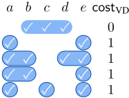
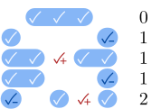
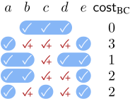
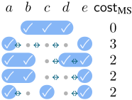
Figure 1: Costs of some ballots under different rules.
such that for each ◁ in f(P) its reverse axis ⃗ ◁ is also in f(P), encoding the idea that the direction of the axis does not matter.
We focus on the family of scoring rules, which we define in analogy to other social choice settings [Myerson, 1995; Pivato, 2013]. Let cost : 2C ×A→R⩾0 be a cost function, so cost(Ai, ◁) is the cost that a ballot Ai ∈ P incurs when the axis ◁ is chosen. Then cost(P, ◁) = ∑Ai∈P cost(Ai, ◁) is the total cost of an axis ◁ for the profile P. An axis rule f is a scoring rule if there is a cost function costf such that f (P ) = arg min◁∈A costf (P, ◁) for all profiles P .
A focus on the class of scoring rules can be justified as an analogue to scoring rules in voting theory, in that every scoring rule satisfies the reinforcement axiom [Young, 1975] which says that if f chooses the same axis ◁ in two disjoint profiles P1 and P2, so that f(P1) ∩ f(P2) ̸= ∅, then the axes it chooses in the combined profile P1 + P2 are exactly the common axes, i.e., f(P1 + P2) = f(P1) ∩ f(P2). However, providing an axiomatic characterization of this class using reinforcement appears to be difficult since the neutrality axiom turns out to be quite weak in our setting. Another motivation for scoring rules is their natural interpretation as maximum likelihood estimators when there is a ground truth axis, as observed by Conitzer et al. [2009] in the voting setting. To see the connection, let ◁ be the ground truth axis, and suppose voters obtain their approval ballots Ai i.i.d. from a probability distribution P(Ai | ◁) (where intuitively ballots are more likely the closer they are to forming an interval of ◁). Then, the likelihood of a profile P is P(P | ◁) = ∏i P(Ai | ◁). To find the axis inducing maximum likelihood, we solve MLE(P) := argmax◁ P(P | ◁) = argmin◁ - ∑i log(P(Ai | ◁)), which is a scoring rule with costs costf (Ai, ◁) = - log(P(Ai | ◁)).
4 Axis Rules
We now introduce five scoring rules. Many are inspired by objective functions proposed for near single-peakedness for rankings [Faliszewski et al., 2014; Escoffier et al., 2021].
The first and simplest rule is called Voter Deletion (VD):
Voter Deletion returns the axes that minimize the number of ballots to delete from the profile P in order to become consistent with it. This rule is a scoring rule based on the cost function costVD such that costVD(A, ◁) = 0 if A is an interval of ◁, and 1 otherwise.
The idea behind this rule is that perhaps some "maverick" voters are "irrational", and should hence be disregarded. The aim is to delete as few maverick voters as possible. Figure 1(a) shows the costs of some ballots under the VD rule, and we clearly observe that the rule gives the same cost to all noninterval ballots.
An intuitive shortcoming of VD is that it does not measure the degree of incompatibility of a given vote with an axis. It does not distinguish ballots that miss just one candidate to be an interval, and an approval ballot in which only the two extreme candidates of the axis are approved. For this reason, more gradual rules might do better.
The first rule in this direction is Minimum Flips (MF) which changes ballots by removing and adding candidates.
MinimumFlips This rule returns the axes that minimize the total number of candidates that need to be removed from and added to approval ballots in order to make the profile linear. It is the scoring rule based on:
The definition of costMF optimizes the choice of the left- and right-most candidates x and y in the ballot after removing and adding candidates, and then counts the number of candidates that were thus removed (first term of the sum) and added (second term). We can equivalently view MF as finding for each vote Ai the interval ballot closest to Ai in Hamming distance, with that distance being the cost of ◁. In another equivalent view, the rule finds the linear profile of minimum total Hamming distance to the input profile, and returns its axes. Figure 1(b) shows the costs of some ballots under the MF rule. Observe that we can obtain an interval by only removing candidates (as in the second ballot), by only adding candidates (as in the third ballot), or by both removing and adding candidates (as in the last ballot).
In many applications, adding approvals seems better motivated than removing them. For example, a voter i might not approve a candidate c because i does not know who c is; fixing this error corresponds to adding a candidate. Choosing to approve some candidate by accident seems less likely. The Ballot Completion (BC) rule implements this thought.
Ballot Completion returns the axes that minimize the number of candidates to add to the ballots to make the profile consistent with it. It uses the cost function
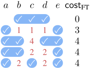
Thus, given a ballot A and an axis ◁, this rule counts all interfering candidates with respect to A and ◁. To see the difference between MF and BC, observe that costBC({a, d}, abcd) = 2 as we need to add b and c to obtain an interval, while costMF({a, d}, abcd) = 1 as we can just remove a. Figure 1(c) shows the costs of some ballots under the BC rule.
In the approval context, BC is the only rule we know of that has already been used in the literature to find an underlying political axis of voters, on the data of experiments conducted during the 2012 and 2017 French presidential elections [Lebon et al., 2017; Baujard and Lebon, 2022]. The axes found by BC were close to the orderings discussed in the media.
The Minimum Swaps (MS) rule modifies the axis rather than the ballots. Given an approval ballot A, the MS rule asks how many candidate swaps we need to perform in an axis ◁ until A becomes an interval of it: the cost costMS(A, ◁) is the minimum Kendall-tau distance between ◁ and an axis ◁′ (the number of swaps of adjacent candidates needed to go from ◁ to ◁′ ) such that A is an interval of ◁′ . For instance, costMS({a, d}, abcd) = 2 because we need to have a next to d on any axis consistent with {a, d}, and we need at least two swaps to obtain this. One can check that this rule is implemented by the following cost function.
Minimum Swaps uses the cost function
Figure 1(d) shows the costs of some ballots under the MS rule. Note that the order in which the swaps are performed matters. Indeed, we need to swap the same pairs for the third and fourth ballot ({c, d} and {d, e}), but we start by swapping c and d in the third ballot and d and e in the fourth ballot.
Finally, the Forbidden Triples (FT) rule is inspired by a proposal by Escoffier et al. [2021]. It counts the number of violations of the interval condition, as defined in Section 3.
Forbidden Triples uses the cost function
Note that there is one forbidden triple for each combination of an interfering candidate and a pair of candidates lying on its left and its right, respectively. Intuitively, this rule looks at the holes in a vote, with larger holes separating many approved candidates counting more. Figure 1(e) shows the costs of some ballots under the FT rule.
The cost functions of our five scoring rules can be related via a chain of inequalities, suggesting that they form a natural collection of rules to study.
Proposition 1. For all ballots A and axes ◁, we have costVD(A, ◁) ⩽ costMF(A, ◁) ⩽ costBC(A, ◁) ⩽ costMS(A, ◁) ⩽ costFT(A, ◁).
If there are m ⩽ 3 candidates, all the rules defined in this section are equivalent (the only possible costs are 0 and 1). If there are m = 4 candidates, VD and MF are equivalent and BC and MS are equivalent. This is because the respective cost functions coincide for m ⩽ 4. For m ⩾ 5, the rules are pairwise non-equivalent; we give examples in the full version. Example 1 shows a profile with m = 4 for which VD, BC, and FT all select different axes.
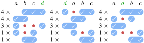
Example 1. Consider the profile P = (4 × {b, c, d}, 4 × {a, b}, 3 × {a, d}, 1 × {a, c}, 1 × {b, c}). On this profile, all rules agree that a ◁ b ◁ c, but they disagree on the position of d. Indeed, ◁1 = abcd is optimal for VD and MF, ◁2 = dabc for BC and MS, and ◁3 = adbc and ◁4 = abdc for FT. Figure 2 shows the profile aligned according to the first three axes.
Problems about recognizing matrices that are almost C1P have long been known to be NP-complete. Hardness of VD and BC is explicitly known (see Booth [1975]), and the reductions only use approval sets of size 2. Hardness of MF, MS, and FT directly follows from the observation that they are equivalent to either VD or BC when maxi |Ai| = 2.
Theorem 1. The VD, MF, BC, MS, and FT rules are NPcomplete to compute, even for profiles in which every ballot approves at most 2 candidates.
A lot of other axis rules could be defined. However, in this paper, we focus on the five rules introduced above, and leave the study of potential other rules to further research. In particular, we think that greedy variants of the rules we introduced are of interest to circumvent computational hardness.
5 Axiomatic Analysis
In this section, we conduct an axiomatic analysis of the rules we introduced. Table 1 summarizes the results of this section.
We start with some basic axioms that all our rules satisfy. The first two are classic symmetry axioms: a rule f is anonymous if whenever two profiles P and P ′ are such that every ballot appears exactly as often in P as in P ′ , then f(P) = f(P ′ ). It is neutral if for every profile P, renaming the candidates in P leads to the same renaming in f(P). The third basic property fundamentally captures the aim of an axis rule: if there are perfect axes, then the rule should return those.
Consistency with linearity. A rule f is consistent with linearity if f(P) = con(P) for all linear profiles P.
If f is a scoring rule and it satisfies these three axioms, we can deduce that its underlying cost function has a certain structure. In particular, it attains its minimum value for consistent axes, it is invariant under reversing the axis, and it is symmetric. We formalize these properties in the full version.
5.1 Stability andMonotonicity
Some rules are more sensitive to changes in information than others. Intuitively, Voter Deletion rarely reacts to changes in the profile, as it only checks whether the ballots are intervals of the axis or not. Thus, a single voter will have little effect on the axes selected. Indeed, for VD, adding a new ballot to the profile cannot completely change the set of optimal solutions. We can formalize this behavior in the following axiom.
| VD | MF | BC | MS | FT | |
|---|---|---|---|---|---|
| Stability | |||||
| Ballot monotonicity | |||||
| Clearance | |||||
| Veto winner centrism | |||||
| Clone-proximity | |||||
| Clone-resistance |
Stability. A rule f satisfies stability if for every profile P and approval ballot A, we have f(P ) ∩ f(P + {A}) ̸= ∅.
Similar axioms were used by [Tydrichov´a [2023], Sec. 4.4.2] for rankings, and by Ceron and Gonzalez [2021] to characterize Approval Voting as a single-winner voting rule. Whether stability is a desirable property depends on the context: while it implies that the rule is robust, it also means that the rule might disregard too much information.
Proposition 2. Stability is satisfied by VD, but not by MF, BC, MS, and FT.
Monotonicity axioms say that if the input changes so as to more strongly support the current output, then the output should stay the same. For our setting, we define monotonicity to say that if some voters complete their ballots by approving all interfering candidates with respect to the current axis ◁, then ◁ should continue being selected. 1
Ballot monotonicity. A rule f satisfies ballot monotonicity if for every profile P , ballot A ∈ P and axis ◁ ∈ f(P) such that A is not an interval of ◁, we still have ◁ ∈ f(P ′ ) for the profile P ′ obtained from P by replacing A by the interval A′ = {x ∈ C : ∃y, z ∈ A s.t. y � x � z}.
VD and BC satisfy this axiom, but the other rules do not.
Proposition 3. Ballot monotonicity is satisfied by VD and BC, but not by MF, MS, and FT.
5.2 Centrists and Outliers
On a high level, good axes should place less popular candidates towards the extremes, where they are less likely to destroy intervals. Conversely, popular candidates are safer to place in the center. We will define two axioms that identify profiles where this expectation is strongest, and that require candidates to be accordingly placed in center or extreme positions.
Our first axiom considers the placement of very unpopular candidates. The axiom is easiest to satisfy by placing them at the extremes, but it does not require doing so in all cases.
Clearance. A rule f satisfies clearance if for every profile P in which candidate x is never approved, all ◁ ∈ f(P) are such that there is no A ∈ P with y, z ∈ A and y ◁ x ◁ z.
Thus, never-approved candidates cannot be interfering.
1 One could define monotonicity in other ways, but we leave the study of those variants to future work.
Proposition 4. Clearance is satisfied by BC, MS, and FT, but not by VD and MF.
While VD and MF always choose some axis that satisfies the clearance condition, they can additionally choose axes which violate this condition, and hence they fail the axiom.
For another way of formalizing the intuition that unpopular candidates should be placed at the extremes, we consider veto profiles in which every ballot has size m- 1, i.e., each voter approves all but one of the candidates. For a veto profile, the only voters who will approve an interval are those who veto a candidate at one extreme of the axis. Since veto profiles do not have any interesting structure, the best candidates to put at the left and right end of the axis are the two candidates with the lowest approval score (i.e., the most vetoed candidates). All of our rules indeed choose only such outcomes.
We can extend this intuition to say that candidates that are vetoed more frequently should be placed at positions closer to the extremes. This would imply that the least vetoed candidate should be placed in the center, so that as few ballots as possible have holes in the center.
Veto winner centrism. A rule f satisfies veto winner centrism if for every veto profile P , the median candidate (or one of the two median candidates if m is even) of every axis ◁ ∈ f(P) has the highest approval score.
Among the rules studied in this paper, only MS and FT satisfy veto winner centrism.
Proposition 5. Veto winner centrism is satisfied by MS and FT, but not by VD, MF, and BC.
In fact, MS and FT always place candidates so that the approval scores are single-peaked.
Clearance and veto winner centrism suggest that MS and FT place unpopular candidates at the extremes, which is also confirmed by our experiments in Section 6. While this generally seems sound, in the political context it can lead to wrong answers: there can be ideologically centrist candidates who don't get many votes due to not being well-known. We leave for future work whether there are rules that can correctly place candidates in these contexts.
5.3 Clones and Resistance to Cloning
We now focus on the behaviour of rules in the presence of essentially identical candidates. We say that a, b ∈ C are clones if for each voter i ∈ V , a ∈ Ai if and only if b ∈ Ai. While perfect clones are rare, studying them gives insights for how rules handle similar candidates.
Intuitively, one would expect clones to be next to each other on any optimal axis. This is captured by the following axiom:
Clone-proximity. A rule f satisfies clone-proximity if for every P in which a, a′ ∈ C are clones, for every axis ◁ ∈ f(P), every candidate x with a◁x◁a′ or a′ ◁x◁a, and every A ∈ P , we have x ∈ A whenever a, a′ ∈ A. Note that x is not necessarily a clone of a and a′ , because x can be approved even if a and a′ are not approved.
Surprisingly, only FT satisfies clone-proximity. All of our rules choose at least one axis where the clones are next to each other, but the rules other than FT may choose extra axes with a violation, as we show in the following result. For instance, in P = (2 × {b, c}, 2 × {c, d}, 1 × {a, a′ , b, d}) the axis a◁b◁c◁d◁a′ in which the clones a and a′ are at opposite extremes is an optimal axis for VD, MF, and BC.
Proposition 6. Clone-proximity is satisfied by FT, but not by VD, MF, BC, and MS.
Inspired by axioms from voting theory [Tideman, 1987], we could require that removing or adding a clone to the profile does not change the result. If we remove a clone from a profile, the restriction of any optimal axis should remain optimal, and adding a clone to a profile should not modify the relative order of the other candidates on any optimal axis. We will need some notation. For a profile P defined on a set C of candidates, we denote by PC′ the restriction of P to a subset of candidates C ′ ⊆ C. We also denote P-c the restriction of the profile to C \ {c} where c ∈ C is a given candidate. Similarly, we define ◁C′ and ◁-c. We can now state the axiom:
Resistance to cloning. A rule f is resistant to cloning if for every P in which a, a′ ∈ C are clones, (1) for all ◁ ∈ f(P), we have ◁-a ∈ f(P-a) and (2) for all ◁∗ ∈ f(P-a), there is an axis ◁ ∈ f(P) with ◁-a = ◁∗ .
Among our rules, only VD is resistant to cloning.
Proposition 7. Resistance to cloning is satisfied by VD, but not by MF, BC, MS, and FT.
These two clone axioms are quite strong: each excludes all but one of our rules. Indeed, we now show that if a scoring rule satisfies neutrality and consistency with linearity, then cloneproximity and resistance to cloning are actually incompatible.
Theorem 2. No neutral scoring rule satisfies resistance to cloning, clone proximity, and consistency with linearity.
We can show that resistance to cloning and ballot monotonicity in fact characterize VD among scoring rules. This not only distinguishes VD from the other four rules, but shows its normative appeal among the entire class of scoring rules.
Theorem 3. Let m ⩾ 6, and let f be a neutral scoring rule. Then f satisfies consistency with linearity, ballot monotonicity, and resistance to cloning if and only if it is VD.
Resistance to cloning can be strengthened to heredity [Tydrichov´a, 2023], a kind of independence of irrelevant alternatives axiom. It states that if we remove any candidate, the rule should return the original axes with that candidate omitted.
Heredity. A rule f satisfies heredity if for every profile P and every subset of candidates C ′ ⊆ C, we have that for each axis ◁ ∈ f(P), there is ◁∗ ∈ f(PC′ ) with ◁C′ = ◁∗ .
However, an easy impossibility theorem shows that no reasonable axis rule can satisfy this axiom.
Proposition 8. No axis rule satisfies heredity and consistency with linearity.
6 Experiments
In this section, we investigate the rules from Section 4 using an experimental analysis, based on synthetic and real datasets. While the rules are hard to compute, for m up to about 12, we can find the best axes in reasonable time using a brute force approach (using pruning and heuristics) and ILP encodings, which we describe in the full version.
Our main aims are (1) to compare our rules to each other, and (2) to compare our rules for approval profiles to two known rules for ranking profiles (VD-rank and FT-rank, see Escoffier et al. 2021). The full version contains more details on the datasets and the experimental results.
6.1 Synthetic Data
To better understand how different rules behave, we tested them on several synthetic data models which sample a linear profile on a ground truth axis and add random noise to it. We then measured the distance of a rule's output to the ground truth. Some of our rules are in fact the MLEs of these noise models, so as predicted they perform well in those cases. However some rules adapted better than others to different noise models. We observed that for all models, our rules tend to push the least approved candidates towards the extremes.
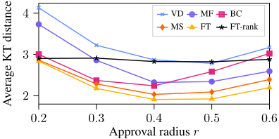
To compare approval-based and ranking-based rules, we introduce the noisy observation model, inspired by random utility models such as the Thurstone-Mosteller model. Each candidate and voter x ∈ C ∪ V is associated with a position p(x) ∈ R on the line. Each voter v estimates the position of each candidate c under independent normal noise: pv(c) = p(c) + N(0, σ) with σ a parameter of the model. Voters approve (resp. rank) candidates based on their estimations. More precisely, the approval set of voter v contains all candidates such that |p(v) - pv(c)| ⩽ r, where the approval radius r is a parameter of the model. The ranking of v is given by decreasing distances between p(v) and pv(c).
The positions p(c) of the candidates describe a ground truth axis. Figure 3 shows the Kendall-tau (KT) swap distance between the axes output by different rule results and the ground truth for σ = 0.3 and r ∈ [0.2, 0.6], and results for other values can be found in the full version. We find that VD-rank is always far from the true axes (at distance 7-8, too much to fit in the chart), and that for most values of σ and r, approval rules actually perform better than FT-rank, returning axes with lower average KT distance to the ground truth. This is surprising, as intuitively rankings provide more information than approvals. However, note that FT-rank is better than approval methods when r is very small or very large, leading to many approval sets having size 0 or 1 (or m), thereby providing no information. FT-rank is also slightly better when σ is small, but in this case all approval rules also have very good performance, with their average KT distances all below 1.

| FT: LO , NPA, PS , LFI, EM, R , LR , DLF, FN , UPR, SP |
| Ipsos: LO , NPA, LFI, PS , EM, R , LR , DLF, FN , SP , UPR |
6.2 The French Presidential Election
We now present the results of our rules on two political datasets: the 2017 and 2022 edition of the online experiment Voter Autrement conducted during the French presidential elections [Bouveret et al., 2018]. In parallel to the actual elections, the participants were invited to express their opinions on candidates using various voting methods, including approval and ranking-based ones. This allows us to compare our axis rules for both settings. After data cleaning, for the 2017 [2022] dataset, we obtained approval preferences of 20076 voters [1379 voters] and preference rankings of 5796 voters [412 voters] over 11 candidates [12 candidates].
We found that all our approval rules returned very similar axes. They mostly differ on the position of less popular candidates (often placed at one of the extremes), and the relative order of candidates within their ideological subgroup (e.g., left-wing candidates). We computed the KT distance between the axes returned by our rules and the ones used by the main 7 polling institutes. All rules return an axis that has a KT distance of less than 5 to at least one poll institute axis (while the worst possible KT distance are 27 and 33 for m = 11 and 12). For instance, the ordering obtained with FT is very similar to the one of the Ipsos institute (see Figure 4). The KT distance between them is 2. Note that the small parties ( LO , NPA, R , UPR, SP ), displayed using small font, are placed at the extremes.
Regarding ranking-based methods, the quality of the axes returned by FT-rank seems comparable to the axes returned by approval rules. The VD-rank axes were much less convincing. This corroborates other observations in the literature. For instance, Sui et al. [2013] ran experiments on 2002 Irish General Election data and found that the VD-rank axis only fit 0.4%-2.9% of voters. Escoffier et al. [2021] ran experiments on a similar French presidential election dataset and also observed that the optimal axis found using VD-rank was very different from the orderings discussed in French media. In our experiments, the optimal VD-rank axes cover less then 4% of voters. For comparison, the approval version of VD returned axes covering more than 60% of voters.
6.3 Supreme Court of the United States
Finally, we used our rules to obtain an ideological ordering of the 9 justices of the Supreme Court of the United States. The dataset is based on the opinions authored and joined by the justices, derived from the Supreme Court Database [Spaeth et al., 2023]. Each opinion, concurrence, or dissent becomes a ballot "approving" the justices that joined in it. The intuition is that justices joining the same opinion share an ideology so should be placed close together.
The problem of ordering the justices has been extensively studied; the standard method used by political analysts is the Martin-Quinn (MQ) method, which uses a dynamic item response theory model [Martin and Quinn, 2002]. A limitation of this model is that it uses only the vote data (whether a justice agreed with the majority or not), while our model can use more fine-grained data about which opinions each justice joined.
| Rule | Avg KT | Correct Median |
|---|---|---|
| VD | 4.94 | 53.8 % |
| MF | 4.22 | 58.5 % |
| BC | 3.68 | 56.9 % |
| MS | 3.55 | 64.6 % |
| FT | 3.43 | 66.2 % |
We compare the axes returned by our rules for 65 terms between 1946 and 2021, removing the years having more than 9 justices involved (e.g., if one is replaced mid-term). Table 2 shows the average KT distance of the axes returned by our rules to the MQ axis. We see that these distances are on average quite low (noting that the worst possible KT distance for m = 9 is 18). Moreover, we observe that the FT rule comes closest, while the VD rule is relatively far away. We also checked how often the axes computed by our rules agreed with the MQ axis on which justice is placed in the median position. This is of particular interest since the median justice tends to be pivotal. All rules agreed with MQ on who was the median justice in more than half of the years. The FT rule agrees most frequently, choosing the same median justice in 66% of terms.
7 FutureWork
There are many promising directions for future work, such as considering methods that output other types of structures, like circular axes (in which the first and last candidates on the axis are next to each other) or embeddings into multiple dimensions, or introducing metric distances between candidates on the axis. An axiomatic approach could provide novel insights for all these problems. Moreover, the methods we present not only return a set of optimal axes, but also their "cost", which provides an indicator of how close a profiles is to be linear. One could try to analyze these methods as rules measuring the degrees of linearity of approval profiles. In addition, one can further investigate the interpretation of scoring rules as maximum likelihood estimators, mentioned at the end of Section 3. In particular, one could develop noise models that give rise to the rules that we study, or develop new natural noise models and (axiomatically) study the rules that they induce, similar to the work of [Tydrichov´a [2023], Section 4.5] for rankings.
Technically, several open questions remain. It would be interesting to obtain an axiomatic characterization of the class of scoring rules using the reinforcement axiom, though this is challenging as the neutrality axiom is quite weak in our setting. It would be useful to design polynomial-time computable rules that produce good outputs, for dealing with many candidates.
Acknowledgments
This work was funded in part by the French government under management of Agence Nationale de la Recherche as part of the "Investissements d'avenir" program, reference ANR19-P3IA-0001 (PRAIRIE 3IA Institute). The authors would like to thank Isabelle Lebon for her help in the early stages of this project, J´erˆome Lang for his helpful comments, and the anonymous reviewers at IJCAI 2024 for helping improve the presentation.
@inproceedings{ijcai2024p305,
  title     = {Comparing Ways of Obtaining Candidate Orderings from Approval Ballots},
  author    = {Delemazure, Théo and Dong, Chris and Peters, Dominik and Tydrichova, Magdalena},
  booktitle = {Proceedings of the Thirty-Third International Joint Conference on
               Artificial Intelligence, {IJCAI-24}},
  publisher = {International Joint Conferences on Artificial Intelligence Organization},
  editor    = {Kate Larson},
  pages     = {2757--2765},
  year      = {2024},
  month     = {8},
  note      = {Main Track},
  doi       = {10.24963/ijcai.2024/305},
  url       = {https://doi.org/10.24963/ijcai.2024/305},
}
TY - CPAPER TI - Comparing Ways of Obtaining Candidate Orderings from Approval Ballots AU - Delemazure, Théo AU - Dong, Chris AU - Peters, Dominik AU - Tydrichova, Magdalena T2 - Proceedings of the Thirty-Third International Joint Conference on Artificial Intelligence, IJCAI-24 PB - International Joint Conferences on Artificial Intelligence Organization PY - 2024 SP - 2757 EP - 2765 DO - 10.24963/ijcai.2024/305 UR - https://doi.org/10.24963/ijcai.2024/305 ER -Copied
Machine-readable versions of this paper, for tools and AI agents:





