Revisiting Causal Discovery from a Complexity-Theoretic Perspective

1 Introduction

Causality has become a crucial topic in AI research for overcoming the limitations of Machine Learning systems that are typically based on correlation. While causal inference focuses on estimating the effect of a known or hypothesized causal relationship, causal discovery (the subject of this paper) aims to uncover new causal relationships directly from data, often without prior hypotheses.

The causal structure over a set of random variables can be explicitly expressed as a causal graph, which is a directed graph whose vertices are the variables, and where an arc X → Y indicates that X is a direct cause of Y . Causal discovery is the problem of identifying as much as possible about the causal graph given a dataset of measurements over the underlying variables; in some cases, part of the causal relationships among the variables is provided from expert knowledge [Ng et al., 2021; Chen et al., 2016; Tsamardinos et al., 2006; Ramaswamy and Szeider, 2022] which can be presented in terms of a super-structure [Perrier et al., 2008; Ordyniak and Szeider, 2013; Ganian and Korchemna, 2021; Gr¨uttemeier and Komusiewicz, 2022], a graph containing all edges which are known or allowed to be part of the causal graph in some orientation.

An important family of algorithms for causal discovery are constraint-based algorithms which work with a (usually very large) set of observational data and repeatedly perform independence checks between pairs of variables, i.e., test X ⊥ Y | Z. Here, it is crucial to distinguish how one models these tests: one commonly assumes these are performed by an oracle which can either (1) determine whether X and Y are conditionally independent via a single query, or (2) test independence under a specific assignment of the conditioning set Z. Here, we take the latter approach-which we from now on refer to as the fine-grained oracle model-as it allows us to more faithfully model settings where, e.g., the data needs to be obtained via on-the-fly experiments or when the amount of data is excessively large. We note that under the fine-grained oracle model, performing independence tests for very large choices of Z becomes infeasible-a fact which also corresponds well to the known unreliability of such independence tests [Wien¨obst and Liskiewicz, 2021; Talvitie and Parviainen, 2020].

The PC algorithm, proposed by Peter and Clarke [Spirtes et al., 2000], is a constraint-based algorithm that had a monumental impact on causal discovery and served as the basis for several other constraint-based algorithms; in fact, it is considered the "default algorithm for attempting causal discovery" [Shalizi, 2023]. The statistical independence check used by the PC algorithm (and many other constraint-based causal discovery algorithms) is based on so-called d-separating sets. Since the running time of the test in the fine-grained oracle model is exponential in the size of the d-separating set, the PC algorithm performs the tests with gradually increasing d-separating sets, starting from checking unconditional independence (which corresponds to checking for the existence of an empty d-separating set).

The PC and other constraint-based algorithms proposed for causal discovery over the last two decades have been refined and analyzed from statistical and empirical perspectives

(see the discussion of related work at the end of the Introduction). However, relatively little is known about the complexitytheoretic foundations of constraint-based causal discovery algorithms in the fine-grained oracle model. We perform the first complexity-theoretic analysis in this more refined setting by attacking the following three fundamental research questions.

Q1 Which structural properties of the causal graph guarantee small d-separating sets between any pair of variables? A small d-separating set is a prerequisite for applying constraintbased causal discovery algorithms efficiently and provides guarantees for their running times.

Q2 How large are the d-separating sets discovered by the PC algorithm compared to smallest d-separating sets? Let us refer to the difference between the size of a d-separating set identified by the PC algorithm and the size of a smallest such set as the "approximation error". The smaller the approximation error, the closer the PC algorithm's time complexity is to the time complexity of an idealistic constraint-based algorithm. antee efficient causal discovery? We consider this question based algorithms that we design to exploit the properties of

• Q3 Which properties of the provided super-structure guarwith respect to the PC algorithm, but also for new constraintthe super-structure better.

1.1 Results

Addressing Q1: We obtain a near-tight characterization of which causal graphs admit a small d-separating set for each pair of vertices. In particular, if the number of edge-disjoint paths between each pair of vertices in the skeleton of the causal graph (i.e., the undirected graph underlying the causal graph) is bounded, then there is a d-separating set between each pair of vertices of bounded size (Theorem 3). At the same time, the statement cannot be strengthened to simply speak of edgedisjoint directed paths (Observation 4) or to the number of vertex-disjoint paths in the skeleton (Theorem 5). Conversely, if a causal graph admits a d-separating set of size at most ℓ for each pair of non-adjacent vertices, then for each pair of nonadjacent vertices, the number of directed vertex-disjoint paths is bounded by the same bound ℓ (Observation 6, Corollary 7). We show that this result is tight in the sense that it cannot be improved to a bound on the number of vertex-disjoint or edge-disjoint paths in the skeleton (Lemma 8) or to a bound on the number of directed edge-disjoint paths in the causal graph (Lemma 9). These results are presented in Section 3.

Addressing Q2: We first observe that no constraint-based causal discovery algorithm can run faster than in time nk , where n is the number of variables and k is the size of a smallest d-separating set between any pair of variables (Lemma 10). In other words, the size of a smallest d-separating set is a hard complexity bound for all constraint-based algorithms.

In the literature, it has been claimed that the PC algorithm will find and use a smallest d-separating set between every pair of variables [Claassen et al., 2013, Subsection 3.1]. We, in fact, show that this is not the case: the PC algorithmmight fail to run efficiently due to failing to find a small d-separating set even when such a set exists. This would be relatively easy to show when expert knowledge is provided, but our construction works even in the base case with no expert knowledge

(i.e., when the super-structure is a complete graph). In particular, we construct a non-trivial class of instances where the PC algorithm only discovers a d-separating set of size linear in the total number of variables, even though there exists a d-separating set of size 3 (Theorem 11). This direction is investigated within our Section 4.

Addressing Q3: We have now seen two obstacles to efficient causal discovery: if the d-separating set is large, then no constraint-based algorithmwill run efficiently, but even if it is small, the PC algorithm might not run efficiently. Here, we consider whether natural graph-theoretic structural restrictions on the super-structure can help us address both of these obstacles to guarantee efficient causal discovery for cases where some (suitable) expert knowledge is available. In particular, we aim to avoid the exponential blowup of nk by designing so-called fixed-parameter algorithms for the problem.

A typical restriction one would consider in the setting of fixed-parameter tractability would be to consider superstructures of bounded treewidth [Robertson and Seymour, 1986]; however, as our first result in this direction we prove that using treewidth (as well as many other more restrictive variants of it that have been used in this context) as a parameter cannot yield fixed-parameter tractability for causal discovery, for any constraint-based algorithm (Corollary 12). On the other hand, we show that the maximum degree in the super-structure is a parameter which guarantees that the PC algorithm will terminate in fixed-parameter time (Theorem 13). Unfortunately, the restriction to super-structures of bounded degree only is very strong, and so this result begs the question of whether tractability can be extended to super-structures of unbounded degree.

We show that by a slight modification of the PC algorithm, we can lift the tractability for the bounded-degree case to parameterizing by the maximum degree within each 2-connected component (Theorem 14); it is worth noting that fixed-parameter tractability for the PC algorithm without our modification cannot be guaranteed in this case (Corollary 15). We conclude by developing a new causal discovery algorithm that guarantees a fixed-parameter running time in a much more general setting-in particular, there it suffices to parameterize by the maximum number of edge-disjoint paths between any pair of variables (Theorem 16)-and again match this with a lower bound showing that the PC algorithm (even the modified one) cannot solve this case efficiently (Corollary 17). This third set of results is presented in Section 5.

1.2 RelatedWork

There are two main approaches to causal discovery: constraintbased and score-based. The complexity of constraint-based causal discovery is well-studied in terms of the number of conditional independence tests. As Claassen et al. [2013] noted, the PC algorithm allows learning causal networks whose node degree is upper-bounded by k via at most n2(k+2) independence tests. Recent works have also explored other constraintbased causal discovery algorithms, including the refinement ED-PC of the PC algorithm by Wien¨obst and Liskiewicz [2021] and MARVEL [Mokhtarian et al., 2021]; the latter achieves nearly-tight bounds in the number of independence tests performed. However, these results do not carry over to the fine-grained oracle model since the algorithms assume the possibility of performing efficient independence tests with large conditioning sets; the sizes of these sets are only upperbounded by the maximal in-degree.

The importance of reducing the sizes of conditioning sets was also mentioned in many other articles (see, e.g., the discussion in the work of Mokhtarian et al. [2022]). For instance, Talvitie and Parviainen [2020] aimed to bound the number of oracle calls and the size of d-separating sets. They did so by considering the so-called moral graph of the hidden causal graph and showed that whenever the moral graph has treewidth at most k, each pair of variables admits a d-separating set of size at most k + 1. This is incomparable to our results addressing Q1: we show that the size of a d-separating set is upper-bounded by a function of the maximum edge-cut of a skeleton of the hidden causal graph (which allows us to obtain strong bounds even for skeletons with high-degree nodes), but it is easy to observe that a bound on the treewidth of the moral graph implies a bound on the degree of the skeleton. An example of an instance where our bounds supersede previous results can be seen, e.g., in Figure 4.

It is known that the smallest d-separating set between X and Y corresponds to the smallest vertex separator in a moral graph of D restricted to ancestors of X and Y [Tian et al., 1998]. We show that this characterization cannot be extended to skeletons (and, therefore, neither to the super-structure setting) by constructing a family of networks with skeletons containing a vertex separator of size 3 between every pair of variables but arbitrarily large smallest d-separating sets between some pair of variables (Theorem 5).

Under the Faithfulness and Causal Markov conditions, causal networks are known to be Bayesian [Mokhtarian et al., 2022]. The parameterized complexity of score-based Bayesian network structure learning was extensively studied in the literature [Ordyniak and Szeider, 2013; Korhonen and Parviainen, 2015; Ganian and Korchemna, 2021; Gr¨uttemeier et al., 2021; Gr¨uttemeier and Komusiewicz, 2022].

2 Preliminaries

We use standard terminology for graph theory [Diestel, 2012]. Let N denote the set of positive integers. We use [i] to denote the set {1, . . . , i}. To obtain our results, we will need to consider undirected graphs as well as directed graphs, i.e., digraphs. We use V (G) to denote the vertex set of a (di)graph G. For a directed graph D, we use A(D) to denote its arc set. The in-neighborhood of a vertex X ∈ V (D) is the set { Y ∈ V (D) | Y X ∈ A(D) }, and the out-neighborhood of X is the set {Y ∈ V (D) | XY ∈ A(D) }. Elements of these sets are called the in- and out-neighbors of X and the sizes of these sets are called the in-degree and out-degree of X, respectively. If H is a subgraph of a (directed or undirected) graph G, we denote this as H ⊆ G. The skeleton (sometimes called the underlying undirected graph) D of a directed graph D is the simple graph obtained by replacing each arc in D with an undirected edge. An edge-cut in D which separates X from Y is a set E of edges such that X and Y lie in different connected components of D - E; we say that E

touches a vertex Z if it contains at least one edge incident to Z. A path between a vertex X1 and a vertex Xn is a non-repeating sequence of vertices X1, . . . ,Xn such that for each pair of vertices Xi and Xi+1, there is an arc XiXi+1 or Xi+1Xi (edge XiXi+1 for an undirected graph). A causal graph is a directed acyclic graph D over a set V (D) of variables (represented as vertices) whose arcs represent causal relationships between these variables. In this paper, we consider variables to range over a finite and fixed domain of size B. A vertex (or variable) Xi is a collider on a path P if the path contains Xi-1 → Xi ← Xi+1; otherwise it is a non-collider [Glymour et al., 2019]. A directed path from X1 to Xn in D is a path which contains an arc XiXi+1 for each pair Xi and Xi+1. If such a path exists, we say that Xn is reachable from X1 or, equivalently, Xn is a descendant of X1 in D. As a special case for n = 1, every variable is reachable from (is a descendant of) itself. A super-structure G is a graph on the same vertex set as the causal graph D which forms a supergraph of the skeleton D of D, i.e., D can be obtained from G by removing some set of edges. In the context of causal discovery, it is used to represent all potential dependencies between variables (known, e.g., from prior or expert knowledge).

Conditional Independence and d-Separation. Let S be a subset of variables in D, and let X and Y be two different variables outside of S. We say that X is d-separated from Y conditional on S if and only if all paths between X and Y in D are blocked by S. A path P is blocked by S if at least one of the following two contions holds:

• P contains a non-collider which is in S, or
• P contains a collider which has no descendants in S.

Assuming the well-established Causal Markov Condition and the Faithfulness Condition, X is d-separated from Y by S if and only if X and Y are conditionally independent given S [Glymour et al., 2019]. Further, we will denote both of these facts (namely, conditional independence and d-separation of X from Y given S) by X ⊥ Y | S.

The PC algorithm. The PC algorithm is one of the basic algorithms used to determine the Markov Equivalence Class (i.e., a partially oriented skeleton) of the causal graph. It receives as input a set V (D) of variables, possibly a superstructure of the (hidden) causal graph over V (D), and an oracle that can check conditional (in)dependencies between variables X, Y w.r.t. a subset of V (D) \ {X, Y }.

In its entirety, the PC algorithm consists of two phases: the first phase (called the learning phase) computes a skeleton, while the second obtains a partial orientation of the skeleton obtained in the first phase. The key distinction is that while the second phase can be implemented as a polynomial-time postproceessing routine, the learning phase can in general take exponential time. Hence, in this complexity-theoretic study we focus our attention solely to the learning phase, which forms the bottleneck in the worst-case running time of the PC algorithm. This phase consists of the following sequence of procedures [Glymour et al., 2019]:

1. Construct a complete undirected graph over the provided set of variables.
2. Eliminate edges between variables that are either unconditionally independent or are known to be independent due to

expert knowledge (non-adjacent in the super-structure).

1. For each pair of variables {X, Y } having an edge between them, and for each variable Z with an edge connected to either of them, eliminate the edge between X and Y if X is conditionally independent of Y given Z.
2. For each pair of variables {X, Y } having an edge between them, and for each pair of variables {Z,W} with edges both connected to X or both connected to Y , eliminate the edge between X and Y if X ⊥ Y | {Z,W}.
3. Continue checking independencies conditional on subsets of variables of size 3, . . . , i until there are no more adjacent pairs X, Y , such that there is a subset of variables of size i such that all of the variables in the subset are adjacent to X or all adjacent to Y .

Let k ≤ i be the maximum size of sets that need to be considered in Step 5 in order for the PC algorithm to discover the whole skeleton of the causal graph. We remark that if k is known in advance, it can be used to provide a basic upper bound on the running time of the PC algorithm, since we may safely stop the process once all sets of size at most k have been checked.

Various variants of the PC algorithm have been proposed over the last two decades [Glymour et al., 2019]. We will refer to all such variants-and in particular, all complete algorithms that are based on checking the conditional independence of pairs of variables in terms of d-separation in a learning phase, followed by an orientation phase (such as the FCI algorithm [Spirtes et al., 2000])-as constraint-based causal discovery algorithms.

Parameterized Complexity. Parameterized complexity theory [Cygan et al., 2015; Downey and Fellows, 2013; Niedermeier, 2006] analyzes the running time of algorithms not only with respect to the input size n, but also to a specified parameter k ∈ N. The high-level idea is to identify parameters which capture the structural properties of instances for computationally challenging problems such that the combinatorial explosion in the running time can be confined to this parameter. The parameterized counterpart to the classical complexity class P is FPT (fixed-parameter tractable), which contains all problems that can be solved by an algorithm running in time f(k) · nO(1) , where f is a computable function. Naturally, not all parameterizations give rise to fixed-parameter tractability for problems of interest, and identifying which do is a central task of parameterized analysis.

3 Characterizing Small d-Separating Sets

The aim of this section is to characterize necessary and sufficient conditions for the existence of bounded-size d-separating sets in a hidden causal graph D. While one would at first glance expect that such conditions would be closely tied to structural properties that depend on the orientation of the arcs in D (and, in fact, some of our results provide precisely such a relationship), here we provide positive results for conditions that are oblivious to the orientation of the arcs, i.e., conditions that solely depend on the undirected skeleton D. There are two reasons for this:

1. It is known to be impossible to identify the exact hidden causal graph D using constraint-based algorithms, but such
2. algorithms can reliably compute D [Eberhardt, 2017, Section 2]. This makes the latter a tangible and guaranteed output of such algorithms.
3. We provide concrete examples and constructions which show that the results linking the existence of bounded-size d-separating sets to undirected structures in D cannot be lifted to analogous directed structures in D.

As a first basic step, it will be useful to provide a lemma that can be seen as an independent short proof of the correctness of the PC algorithm. For two distinct variables X and Y in D, let DXY and DXY be the subgraphs of D and D respectively induced on the vertices of the set of all undirected paths between X and Y in D. For the following, it will be useful to recall that the causal graphs considered here are acyclic.

Lemma 1. Let X and Y be distinct and non-adjacent variables such that X is not reachable from Y in D. Let S be the set of all in-neighbors of Y in DXY . Then X ⊥ Y | S.

Lemma 1 immediately implies that if the causal graph has indegree ℓ, then every pair of variables admits a d-separating set of size at most ℓ. In particular, bounded maximum in-degree in D-and hence also bounded maximum degree in D-is a sufficient condition for the existence of small d-separating sets. Naturally, such a condition is far from necessary: for instance, the class of simple stars with all edges oriented towards the center has arbitrarily large maximum in-degree even though each pair of non-adjacent variables admits a d-separating set of size 0.

As our next task, we will provide a stronger sufficient condition on D for the existence of small d-separating setsspecifically, the existence of a bounded number of edgedisjoint paths between each pair of variables. The next lemma provides the first step towards this goal:

Lemma 2. Let X and Y be non-adjacent vertices in D such that X is not reachable from Y in D. Assume that D admits an edge-cut of size k which separates X and Y and does not touch X. Then X and Y can be d-separated by a set of size at most 2k in D.

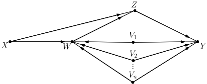
We note that it is crucial that the edge-cut considered in Lemma 2 does not touch X: Figure 1 depicts a causal graph admitting an edge-cut {XZ,XW} of size two, but requires large d-separating set for X and Y .

Interestingly, when aiming for a sufficient condition that would guarantee the existence of small d-separating sets between all pairs of variables, we show that the existence of arbitrary edge-cuts of bounded size is sufficient (regardless of which variables they touch).

Theorem 3. If every pair of vertices X and Y can be separated in D by an edge-cut of size at most k, then every pair of non-adjacent variables can be d-separated in D by a set of size at most 2k2 .

Notice that the bound above is imposed on the number of undirected edge-disjoint paths. By contrast, restricting the number of directed edge-disjoint paths does not suffice: as a simple example, consider a causal graph Ln that consists of two variables X and Y plus n vertex-disjoint paths of length 2 between them, where every vertex other than X and Y is a source. In particular, X and Y are sinks.

Observation 4. Ln does not contain a directed path between any pair of non-adjacent variables, but the only d-separating set for X and Y has size n.

However, this still raises the question of whether Theorem 3 could be strengthened by simply requiring the existence of a vertex-separator of size at most k (instead of having an edgecut of size at most k) between each pair of variables. Below, we answer this in the negative:

Theorem 5. There exists a family {Di : i ∈ N} of causal graphs with |V (Di)| = O(4i ), i ∈ N, such that each Di contains a pair of non-adjacent variables with no d-separating set of size smaller than 2i-1 +1, and yet each pair of variables in Di admits a vertex separator of size 3.

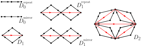
Proof Sketch. For convenience, let us define D0 to simply be a causal graph consisting of a single arc. If the edge begins in X and ends in Y , we say that D0 has orientation XY . We construct the family by induction; to this end, let us assume that the causal graph Di, i ∈ N∪{0}, has already been defined and has a special pair of vertices called its orientation.

For the construction itself, take two vertex-disjoint copies of Di with orientations XR and R′Y and glue them together by identifying R and R′ , and denote the obtained graph as Drepeat i . Take another two vertex-disjoint copies of Di with orientations M ′X′ and MY ′ and glue them together by identifying M and M ′ , and denote the graph as Dmirror i . Finally, glue together Drepeat i and Dmirror i by identifying X′ with X and Y ′ with Y . The resulting graph is Di+1 with orientation XY . An illustration of the construction-which may be viewed as "fractal" in nature-is provided in Figure 2.

To complete the proof, it now remains to establish the fol-

lowing two claims:

Claim 1. For every i ∈ N, Di admits a vertex separator of size at most 3 between any pair of vertices.

Claim 2. For every i ∈ N, the causal graph Di with orientation XY contains no d-separating set between X and Y of size smaller than 2i-1 + 1.

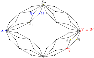
The proof of Claim 1 is based on case analysis for all pairs of variables, and is illustrated on Figure 3. The key insight underlying the proof of Claim 2 is that at each step fromDi to Di+1, the size of a minimum d-separating set can be shown to increase by a factor of 2.

Theorems 3 and 5 imply that while having a bounded number of undirected edge-disjoint paths between variables guarantees the presence of a bounded-size d-separating set, this is not the case for undirected vertex-disjoint paths. Hence, having a bounded number of undirected edge-disjoint paths can be seen as a sufficient condition for the existence of a bounded-size d-separating set. Our aim in the rest of this section is to identify a condition which is necessary.

We begin by making a simple observation concerning a necessary condition tied to the hidden causal graph (as opposed to the skeleton). In particular, since a d-separating set must intersect each directed path between a pair of variables in the causal graph, we obtain:

Observation 6. If a causal graph D admits a d-separating set of size k for each pair of non-adjacent variables, then for each pair of non-adjacent variables the number of directed vertex-disjoint paths is bounded by the same bound k.

In terms of conditions on the actual skeleton D, we note the following. If the number of vertex-disjoint paths between two non-adjacent variables X and Y in D is large, then there exists an acyclic orientation of D with no small d-separating set between X and Y (this occurs, e.g., when all of the X-Y paths are oriented from X to Y ). Hence, having a small number of vertex-disjoint paths between each pair of non-adjacent variables is necessary to guarantee that every orientation of D admits a small d-separating set. In other words:

Corollary 7. Let D be an undirected graph. Assume that, in every acyclic orientation D of D, every pair of non-adjacent variables can be d-separated in D by a set of size k. Then every pair of non-adjacent variables can be separated in D by a vertex separator of size at most k.

Finally, the fact that Corollary 7 references every orientation D of D is crucial. Indeed:

Lemma 8. There exists a family of undirected graphs H = {X i | i ∈ N} with the following properties: (I) Each X i admits an acyclic orientation Xi where every pair of nonadjacent variables can be d-separated by a set of size 0, and (II) X i contains a pair of non-adjacent variables A, B whose minimum vertex separator has size i.

As the final result in this section, we also exclude the possibility of generalizing Observation 6 to a bound on the number of directed edge-disjoint paths (as opposed to a bound on the number of directed vertex-disjoint paths).

Lemma 9. There exists a family {D′i : i ∈ N} of causal graphs with |V (D′i )| = O(4i ), i ∈ N, such that each Di contains 2i directed edge-disjoint paths between some pair of non-adjacent variables, and yet each pair of non-adjacent variables can be d-separated by a set of size at most 3.

Proof Sketch. For every i ∈ N0, we define the causal graph D′i as follows. The skeleton of D′i coincides with the skeleton of Di from Theorem 5, and if such Di has orientation XY , in D′i we orient all the arcs on every path from X and Y towards Y . In particular, D′i+1 can be obtained by gluing together 4 copies of D′i , i ∈ N0. To complete the proof, it suffices to show that there are constant-sized d-separating sets between each pair of variables in D′i ; at that point, the lemma follows from the fact that each causal graph D′i consists of 2i edge-disjoint directed paths from X to Y .

4 Limits of Tractability for the PCAlgorithm

While the previous section was aimed at identifying necessary and sufficient conditions for the existence of a small dseparating set, having a small d-separating set itself is merely a necessary condition for efficient causal discovery. Indeed, in this section we show that the existence of a small d-separating set cannot on its own guarantee efficient running times for causal discovery.

We begin with a lower bound ruling out fixed-parameter causal discovery by any constraint-based algorithm:

Lemma 10. There exists a class of causal graphs H = {Di,k | i, k ∈ N; k ≤ i } such that: (I) each Di,k contains i + 3 vertices, (II) each Di,k has a single pair X, Y of nonadjacent vertices with a d-separating set of size k, and (III) on each Di,k, no constraint-based algorithm can determine whether X and Y are conditionally independent in time less than Θ(nk-1 ).

While Lemma 10 may already seem disheartening, the lower bound it provides only becomes truly problematic as k grows above a small constant. In other words, at this point it would still seem plausible that the PC algorithm achieves a running time of, e.g., nO(k) , where k is the size of the largest d-separating set in the causal graph. As our second result in this section, we show that the situation is in fact much worsethere is a class of causal graphs for which the PC algorithm will necessarily run in exponential time, even though all pairs of variables admit very small d-separating sets between them.

Theorem 11. For each n ≥ 2, there exists a causal graph Tn on O(2n ) vertices such that Tn admits d-separating sets of size at most 3 between every pair of non-adjacent variables, but the PC algorithm only discovers a d-separating set of size 2n + 2 for at least one pair of variables.

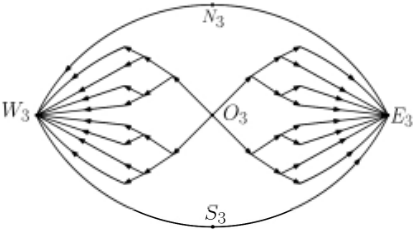
Proof Sketch. To obtain Tn, we start from two full binary trees T 1 n and T 2 n with 2n leaves each, where all the arcs are oriented from the roots to the leaves. We glue T 1 n and T 2 n together at their roots and denote the resulting common root by On. Moreover, we introduce a variable Wn and add an incoming arc to it from every leaf of T 1 n . Symetrically, we introduce a variable En and add an incoming arc to it from every leaf of T 2 n . Finally, we add two variables Nn and Sn along with out-going arcs to X and Y from both of them, see Figure 4 for an illustration.

Now, let us analyze how the PC algorithm will discover the d-separating sets in Tn. In the first stage, it searches for d-separating sets of size 0, which will disconnect Sn and Nn from all the other vertices except En and Wn. It will then proceed by searching for d-separating sets in the neighborhoods of each pair of variables which still have an edge between them, and one can show that this results in the discovery of Tn plus one additional edge WnEn by the time it completes its check for d-separating sets of size at most 3. However, to eliminate this final edge, the PC algorithm will need to use a d-separating set containing Nn, Sn and all the leaves of T 1 n or T 2 n . Such a set has size at least 2n + 2.

5 Utilizing the Super-Structure for Fixed-Parameter Algorithms

In our final section, we show that the lower bounds arising from Lemma 10 and Theorem 11 can both be circumvented if we are provided with a super-structure possessing suitable structural properties. In particular, our aim is to show that causal discovery can be carried out in fixed-parameter time not with respect to the size of a maximum d-separating set (as this was ruled out in Lemma 10), but instead with respect to a structural measure of a provided super-structure.

A natural graph-theoretic measure of the super-structure is the well-established treewidth-a fundamental graph parameter which intuitively captures the "tree-likeness" of a graph [Robertson and Seymour, 1986]. However, we can immediately rule out the use of treewidth (and also many other related graph parameters) by recalling the graph class L = {Li | i ∈ N} used in Observation 4. Indeed, X and Y form a vertex cover of each graph Li ∈ L, and hence all graphs in that class have treewidth at most 2. However, the only d-separating set between X and Y has size i. Thus, by setting L′i to be a super-structure for Li that contains each edge in Li plus the edge XY , we obtain the corollary below. In particular, each Li consists of X, Y , and a set of i sources adjacent to both X and Y , and L′i adds a "superfluous" edge XY to the skeleton of Li.

Corollary 12. For every i ∈ N, there exists a super-structure L′i of Li with a vertex cover of size 2 such that no constraintbased causal discovery algorithm can compute the skeleton of the hidden causal graph Li in time less than Bi .

We remark that the same construction rules out efficient algorithms based on not only the treewidth and the vertex cover number, but also pathwidth, treedepth [Nesetril and de Mendez, 2012], tree-cut width [Ganian et al., 2022] and a range of other graph parameters typically used to achieve fixed-parameter tractability. However, as we will see in the rest of the section, there are natural structural properties of the super-structure which guarantee efficient causal discovery. The first such property is the maximum degree in the superstructure. It may be worth noting that it is exceedingly rare for a computational problem to be fixed-parameter tractable w.r.t. the maximum degree and yet intractable w.r.t. parameters such as the vertex cover number.

Theorem 13. If the PC algorithm is provided an n-variable super-structure G of maximum degree k, then it will discover the skeleton D of the hidden causal graph in time 2kBkO(nk), where B is the size of domain.

Next, we show that the tractability result of Theorem 13 can be extended to the setting where only the maximum degree of each 2-connected component is bounded. To this end, we define a new constraint-based algorithm PC∗ . For a superstructure G and two variables X, Y ∈ V (G), let GXY be the subgraph of G induced by all paths between X and Y in G. PC∗ takes G (which may, in the worst case, be the complete graph) as input and proceeds similarly to the PC algorithm, with only a single modification: while looking for potential d-separating sets for X and Y , it only checks those subsets of neighbors of Y that belong to GXY .

Theorem 14. Given a super-structure G of D over n variables, PC∗ computes the skeleton of D in time 2kBkO(nk), where k is the maximum degree over all 2-connected components of G.

Even though the difference between the PC and PC∗ algorithms might seem rather subtle, the latter immediately extends the class of instances for which the skeleton can be computed efficiently. This can be illustrated, e.g., on the class {Lnk | n, k ∈ N} of causal graphs obtained from the graphs Lk (cf. Observation 4) by introducing n-k new in-neighbors of X and n - k new in-neighbors of Y .

Corollary 15. If Lnk is a hidden causal graph and G contains the only extra edge between its pair of high-degree vertices, then the PC algorithm requires Ω(nk-1 ) iterations to eliminate the single superfluous edge in G, while the PC* algorithm computes the skeleton in time 2kBkO(nk).

As our final contribution, we provide a new causal discovery algorithm called PCcut that features fixed-parameter runtime guarantees not only on all instances where the PC and PC* algorithms do, but also on more general classes of inputs. To this end, it will be useful to recall that a bound on the size of smallest edge-cuts between each pair of variables is a sufficient condition for the existence of small d-separating sets (see Theorem 3). While causal graphs with this property need not be efficiently discoverable by constraint-based algorithms, this changes when dealing with a provided super-structure.

The PCcut algorithm alters the original PC algorithm by testing conditional independence via subsets selected from a smallest edge-cut between the variables X, Y , instead of simply checking the neighborhood of these two variables. More precisely, we define the PCcut algorithm as follows. It begins by performing the same initial two steps as the PC algorithm (see Section 2). Afterwards, it performs a subroutine that starts with j := 1 and increments this up to a value of 2k2 , where k upper-bounds the size of a smallest edge-cut. For each choice of j, it runs over all ordered pairs of adjacent variables, and for each such pair (X, Y ) it computes an edge-cut E of minimum size between X and Y in the graph computed so far (but without the edge XY ) that does not touch X (this can be done, e.g., via the Ford-Fulkerson algorithm where we make the edges incident to X undeletable). Let S E be the set of variables incident to the edges in E. We now perform essentially the same procedure the PC algorithm originally performs over the neighborhood of X and Y , but on the set S E ; in particular, for all subsets S of S E of size j, we test whether X ⊥ Y | S and if this test succeeds we eliminate the edge XY .

Theorem 16. When given a super-structure G of an n-variable causal graph D such that each pair of variables can be separated by an edge-cut of size at most k in G, the PCcut algorithm will compute the skeleton D of D in time at most 22k2 B2k2 O(nk).

We conclude this section by noting that there exist classes of inputs where PCcut will outperform both the PC and PC* algorithms by an arbitrarily large factor. For instance, this occurs on the class of causal graphs depicted in Figure 4.

Corollary 17. If Tn is a hidden causal graph and G contains the only extra edge between its pair of high-degree vertices, PC and PC* need 2Ω(2n ) iterations to eliminate the single extra edge, while PCcut computes the skeleton in time BO(1)n.

6 Concluding Remarks

Our results yield deep insights into how causal graph structures impact constraint-based causal discovery algorithms. We have provided detailed near-tight characterizations of causal graphs allowing small d-separating sets, identified obstacles for the PC algorithm to run efficiently, and established fixedparameter tractability by exploiting properties of the superstructure. However, it remains open whether a skeleton with many edge-disjoint paths between variable pairs implies the existence of a large d-separating set orientation. Although the immediate practical implications of our results may be limited, we believe they will inspire novel approaches for the foundational as well as empirical aspects of causal discovery.

Acknowledgments

The authors are grateful for and acknowledge support from the Austrian Science Fund (FWF, Projects 10.55776/Y1329, 10.55776/P36688, 10.55776/P36420, and 10.55776/COE12) as well as from the Vienna Science and Technology Fund (WWTF, Project ICT22-029).