
Learning Big Logical Rules by Joining Small Rules
Proceedings of the Thirty-Third International Joint Conference on Artificial Intelligence. Main Track. Pages 3430-3438.
https://doi.org/10.24963/ijcai.2024/380
Keywords
- Machine Learning: ML: Symbolic methods
- Knowledge Representation and Reasoning: KRR: Logic programming
Abstract
A major challenge in inductive logic programming is learning big rules. To address this challenge, we introduce an approach where we join small rules to learn big rules. We implement our approach in a constraint-driven system and use constraint solvers to efficiently join rules. Our experiments on many domains, including game playing and drug design, show that our approach can (i) learn rules with more than 100 literals, and (ii) drastically outperform existing approaches in terms of predictive accuracies.
- [Bacchus et al., 2021] Fahiem Bacchus, Matti Järvisalo, and Ruben Martins. Maximum satisfiabiliy. In Armin Biere, Marijn Heule, Hans van Maaren, and Toby Walsh, editors, Handbook of Satisfiability -Second Edition, volume 336 of Frontiers in Artificial Intelligence and Applications, pages 929-991. IOS Press, 2021.
- [Bembenek et al., 2023] Aaron Bembenek, Michael Green- berg, and Stephen Chong. From SMT to ASP: Solver-based approaches to solving datalog synthesis-as-rule-selection problems. Proc. ACM Program. Lang., 7(POPL), jan 2023.
- [Biere et al., 2021] Armin Biere, Marijn Heule, Hans van Maaren, and Toby Walsh, editors. Handbook of Satisfi- ability -Second Edition, volume 336 of FAIA. IOS Press, 2021.
- [Biere et al., 2023] Armin Biere, Mathias Fleury, and Flo- rian Pollitt. CaDiCaL, vivinst, IsaSAT, Gimsatul, Kissat, and TabularaSAT entering the SAT Competition 2023. In Proc. SAT Competition 2023: Solver, Benchmark and Proof Checker Descriptions, volume B-2023-1 of Department of Computer Science Report Series B, pages 14-15. University of Helsinki, 2023.
- [Blockeel and De Raedt, 1998] Hendrik Blockeel and Luc De Raedt. Top-down induction of first-order logical deci- sion trees. Artificial intelligence, 101(1-2):285-297, 1998.
- [Bramley et al., 2018] Neil Bramley, Anselm Rothe, Josh Tenenbaum, Fei Xu, and Todd M. Gureckis. Grounding compositional hypothesis generation in specific instances. In Proceedings of the 40th Annual Meeting of the Cognitive Science Society, CogSci 2018, 2018.
- [Bunel et al., 2018] Rudy Bunel, Matthew Hausknecht, Jacob Devlin, Rishabh Singh, and Pushmeet Kohli. Leveraging grammar and reinforcement learning for neural program synthesis. arXiv preprint arXiv:1805.04276, 2018.
- [Castillo and Wrobel, 2002] Lourdes Pena Castillo and Ste- fan Wrobel. Macro-operators in multirelational learning: a search-space reduction technique. In European Conference on Machine Learning, pages 357-368. Springer, 2002.
- [Chollet, 2019] Franc ¸ois Chollet. On the measure of intelli- gence. CoRR, 2019.
- [Corapi et al., 2011] Domenico Corapi, Alessandra Russo, and Emil Lupu. Inductive logic programming in answer set programming. In Inductive Logic Programming -21st International Conference, pages 91-97, 2011.
- [Costa et al., 2003] Vítor Santos Costa, Ashwin Srinivasan, Rui Camacho, Hendrik Blockeel, Bart Demoen, Gerda Janssens, Jan Struyf, Henk Vandecasteele, and Wim Van Laer. Query transformations for improving the efficiency of ILP systems. Journal of Machine Learning Research, pages 465-491, 2003.
- [Cropper and Dumančić, 2020] Andrew Cropper and Sebasti- jan Dumančić. Learning large logic programs by going beyond entailment. In Proceedings of the Twenty-Ninth International Joint Conference on Artificial Intelligence, IJCAI 2020, pages 2073-2079, 2020. IJCAI
- [Cropper and Hocquette, 2023] Andrew Cropper and Céline Hocquette. Learning logic programs by combining pro- grams. In ECAI 2023 -26th European Conference on Artificial Intelligence, volume 372, pages 501-508. IOS Press, 2023.
- [Cropper and Morel, 2021] Andrew Cropper and Rolf Morel. Learning programs by learning from failures. Machine Learning, 110(4):801-856, 2021.
- [Cropper et al., 2020] Andrew Cropper, Richard Evans, and Mark Law. Inductive general game playing. Machine Learning, 109(7):1393-1434, 2020.
- [Cropper et al., 2022] Andrew Cropper, Sebastijan Du- mančić, Richard Evans, and Stephen H. Muggleton. In- ductive logic programming at 30. Machine Learning, 111(1):147-172, 2022.
- [Devlin et al., 2017] Jacob Devlin, Jonathan Uesato, Surya Bhupatiraju, Rishabh Singh, Abdel-rahman Mohamed, and Pushmeet Kohli. Robustfill: Neural program learning under noisy i/o. In International conference on machine learning, pages 990-998. PMLR, 2017.
- [Evans and Grefenstette, 2018] Richard Evans and Edward Grefenstette. Learning explanatory rules from noisy data. Journal of Artificial Intelligence Research, pages 1-64, 2018.
- [Evans et al., 2021] Richard Evans, José Hernández-Orallo, Johannes Welbl, Pushmeet Kohli, and Marek J. Sergot. Making sense of sensory input. Artificial Intelligence, page 103438, 2021.
- [Ferilli, 2016] Stefano Ferilli. Predicate invention-based spe- cialization in inductive logic programming. Journal of Intelligent Information Systems, 47(1):33-55, 2016.
- [Finn et al., 1998] Paul Finn, Stephen Muggleton, David Page, and Ashwin Srinivasan. Pharmacophore discovery using the inductive logic programming system progol. Ma- chine Learning, 30(2):241-270, 1998.
- [Galárraga et al., 2015] Luis Galárraga, Christina Teflioudi, Katja Hose, and Fabian M. Suchanek. Fast rule mining in ontological knowledge bases with AMIE+. VLDB J., 24(6):707-730, 2015.
- [Genesereth and Björnsson, 2013] Michael Genesereth and Yngvi Björnsson. The international general game play- ing competition. AI Magazine, 34(2):107-107, 2013.
- [Hocquette et al., 2024] Céline Hocquette, Andreas Niska- nen, Matti Järvisalo, and Andrew Cropper. Learning MDL logic programs from noisy data. In AAAI, 2024.
- [Ignatiev et al., 2018] Alexey Ignatiev, Antonio Morgado, and Joao Marques-Silva. PySAT: A Python toolkit for prototyping with SAT oracles. In International Conference on Theory and Applications of Satisfiability Testing, pages 428-437. Springer, 2018.
- [Kaminski et al., 2019] Tobias Kaminski, Thomas Eiter, and Katsumi Inoue. Meta-interpretive learning using hex- programs. In Proceedings of the Twenty-Eighth Interna- tional Joint Conference on Artificial Intelligence, IJCAI 2019, pages 6186-6190, 2019.
- [Law et al., 2014] Mark Law, Alessandra Russo, and Krysia Broda. Inductive learning of answer set programs. In Logics in Artificial Intelligence -14th European Conference, JELIA 2014, pages 311-325, 2014.
- [Liffiton and Sakallah, 2008] Mark H. Liffiton and Karem A. Sakallah. Algorithms for computing minimal unsatisfiable subsets of constraints. J. Autom. Reason., 40(1):1-33, 2008.
- [Lloyd, 2012] John W Lloyd. Foundations of logic program- ming. Springer Science & Business Media, 2012.
- [Manthey et al., 2014] Norbert Manthey, Tobias Philipp, and Peter Steinke. A more compact translation of pseudo- Boolean constraints into CNF such that generalized arc consistency is maintained. In Carsten Lutz and Michael Thielscher, editors, KI 2014, volume 8736 of LNCS, pages 123-134. Springer, 2014.
- [Mihalkova et al., 2007] Lilyana Mihalkova, Tuyen N. Huynh, and Raymond J. Mooney. Mapping and revis- ing markov logic networks for transfer learning. In Proceedings of the Twenty-Second AAAI Conference on Artificial Intelligence, July 22-26, 2007, Vancouver, British Columbia, Canada, pages 608-614. AAAI Press, 2007.
- [Muggleton, 1991] Stephen Muggleton. Inductive logic pro- gramming. New Generation Computing, 8(4):295-318, 1991.
- [Muggleton, 1995] Stephen H. Muggleton. Inverse en- tailment and Progol. New Generation Computing, 13(3&4):245-286, 1995.
- [Piotrów, 2020] Marek Piotrów. UWrMaxSat: Efficient solver for MaxSAT and pseudo-Boolean problems. In 2020 IEEE 32nd International Conference on Tools with Artifi- cial Intelligence (ICTAI), pages 132-136, 2020.
- [Quinlan, 1990] J. Ross Quinlan. Learning logical definitions from relations. Machine Learning, pages 239-266, 1990.
- [Raghothaman et al., 2020] Mukund Raghothaman, Jonathan Mendelson, David Zhao, Mayur Naik, and Bernhard Scholz. Provenance-guided synthesis of datalog programs. Proc. ACM Program. Lang., 4(POPL):62:1-62:27, 2020.
- [Shapiro, 1983] E.Y. Shapiro. Algorithmic program debug- ging. 1983.
- [Shi et al., 2022] Kensen Shi, Hanjun Dai, Kevin Ellis, and Charles Sutton. Crossbeam: Learning to search in bottom- up program synthesis. In International Conference on Learning Representations, 2022.
- [Si et al., 2019] Xujie Si, Mukund Raghothaman, Kihong Heo, and Mayur Naik. Synthesizing datalog programs using numerical relaxation. In Proceedings of the Twenty-Eighth International Joint Conference on Artificial Intelligence, IJCAI 2019, pages 6117-6124, 2019. IJCAI
- [Silverstein and Pazzani, 1991] Glenn Silverstein and Michael J Pazzani. Relational clichés: Constraining constructive induction during relational learning. In Machine Learning Proceedings 1991, pages 203-207. Elsevier, 1991.
- [Srinivasan, 2001] Ashwin Srinivasan. The ALEPH manual. Machine Learning at the Computing Laboratory, Oxford University, 2001.
- [Xu et al., 2023] Yudong Xu, Wenhao Li, Pashootan Vaezipoor, Scott Sanner, and Elias B Khalil. LLMs and the abstraction and reasoning corpus: Successes, failures, and the importance of object-based representations. arXiv preprint arXiv:2305.18354, 2023.
References were extracted automatically from the PDF and may contain errors.
Full text extracted automatically from the PDF; figures, tables and equations may differ. The PDF is the version of record.
1 Introduction
Zendo is an inductive reasoning game. One player, the teacher, creates a secret rule that describes structures. The other players, the students, try to discover the secret rule by building structures. The teacher marks whether structures follow or break the rule. The first student to correctly guess the rule wins. For instance, for the positive examples shown in Figure 1, a possible rule is "there is a blue piece".

To use machine learning to play Zendo, we need to learn explainable rules from a small number of examples. Although crucial for many real-world problems, many machine-learning approaches struggle with this type of learning [Cropper et al., 2022]. Inductive logic programming (ILP) [Muggleton, 1991] is a form of machine learning that can learn explainable rules from a small number of examples. For instance, for the examples in Figure 1, an ILP system could learn the rule:
This rule says that the relation zendo holds for the structure S when there is a blue piece B.
Suppose we also have the three negative examples shown in Figure 2. Our previous rule incorrectly entails the first and second negative examples, as they have a blue piece. To entail all the positive and no negative examples, we need a bigger rule, such as:

This rule says that the relation zendo holds for a structure when there is a blue piece, a red piece, and a green piece.
Most ILP approaches can learn small rules, such as h1. However, many struggle to learn bigger rules, such as h2 1 . This limitation noticeably holds for approaches which precompute all possible rules and search for a subset of them [Corapi et al., 2011; Law et al., 2014; Kaminski et al., 2019; Si et al., 2019; Raghothaman et al., 2020; Evans et al., 2021; Bembenek et al., 2023]. As they precompute all rules, these approaches struggle to learn rules with more than a few literals.
To address this limitation, we introduce an approach that learns big rules by joining small rules. The idea is to first find small rules where each rule entails some positive and some negative examples. We then search for conjunctions of these small rules such that each conjunction entails at least one positive example but no negative examples.
To illustrate our idea, consider our Zendo scenario. We find rules that entail at least one positive example, such as:
Each of these rules entails at least one negative example. Therefore, we search for a subset of these rules where the intersection of the logical consequences of the subset entails at least one positive example and no negative examples. The set of rules {r1, r2, r3} satisfies these criteria. We therefore form a hypothesis from the conjunction of these rules:
1 A rule of size 7 is not especially big but for readability we do not use a bigger rule in this example. In our experiments, we show we can learn similar rules with over 100 literals.
The hypothesis h3 entails all the positive but none of the negative examples and has the same logical consequences (restricted to zendo/1 atoms) as h2.
The main benefit of our approach is that we can learn rules with over 100 literals, which existing approaches cannot. Our approach works because we decompose a learning task into smaller tasks that can be solved separately. For instance, instead of directly searching for a rule of size 7 to learn h2, we search for rules of size 3 (r1 to r3) and try to join them to learn h3. As the search complexity of ILP is usually exponential in the size of the program to be learned, this reduction can substantially improve learning performance. Moreover, because we can join small rules to learn big rules of a certain syntactic form, we can eliminate splittable rules from the search space. We formally define a splittable rule in Section 4, but, informally, the body of a splittable rule can be decomposed into independent subsets, such as the body of h2 in our Zendo scenario.
To explore our idea, we build on learning from failures (LFF) [Cropper and Morel, 2021], a constraint-driven ILP approach. We extend the LFF system COMBO [Cropper and Hocquette, 2023] with a join stage to learn programs with big rules. We develop a Boolean satisfiability (SAT) [Biere et al., 2021] approach to find conjunctions in the join stage. We call our implementation JOINER.
Novelty and Contributions. Our main contribution is the idea of joining small rules to learn big rules which, as our experiments on many diverse domains show, can improve predictive accuracies. Overall, our main contributions are:
- We introduce an approach which joins small rules to learn big rules.
- We implement our approach in JOINER, which learns optimal (textually minimal) and recursive programs. We prove the correctness of JOINER (Theorem 1).
- We experimentally show on several domains, including game playing, drug design, and image reasoning, that our approach can (i) learn rules with more than 100 literals, and (ii) drastically outperform existing approaches in terms of predictive accuracy.
2 RelatedWork
Program synthesis. Several approaches build a program one token at a time using an LSTM [Devlin et al., 2017; Bunel et al., 2018]. CROSSBEAM [Shi et al., 2022] uses a neural model to generate programs as the compositions of seen subprograms. CROSSBEAM is not guaranteed to learn a solution if one exists and can only use unary and binary relations. By contrast, JOINER can use relations of any arity.
Rule mining. AMIE+ [Gal´arraga et al., 2015] is a prominent rule mining approach. In contrast to JOINER, AMIE+ can only use unary and binary relations and struggles to learn rules with more than 4 literals.
ILP. Top-down ILP systems [Quinlan, 1990; Blockeel and De Raedt, 1998] specialise rules with refinement operators [Shapiro, 1983]. Some systems join literals for look-ahead search to improve performance [Silverstein and Pazzani, 1991; Castillo and Wrobel, 2002]. Because they learn a single rule at a time and add at most a couple of literals at each step, these systems struggle to learn recursive and optimal programs. Recent approaches overcome these issues by formulating the search as a rule selection problem [Corapi et al., 2011; Evans and Grefenstette, 2018; Kaminski et al., 2019; Si et al., 2019; Raghothaman et al., 2020; Evans et al., 2021; Bembenek et al., 2023]. These approaches precompute all possible rules (up to a maximum rule size) and thus struggle to learn rules with more than a few literals. While these approaches could precompute non-splittable rules only and use our join algorithm to find big rules, they would still struggle to scale to big rules. By contrast, we avoid enumeration and use constraints to soundly prune rules.
Many rules. COMBO [Cropper and Hocquette, 2023] searches for a disjunction of small programs that entails all the positive examples. COMBO learns optimal and recursive programs and large programs with many rules. However, it struggles to learn rules with more than 6 literals. Our approach builds on COMBO and can learn rules with over 100 literals.
Big rules. Inverse entailment approaches [Muggleton, 1995; Srinivasan, 2001] can learn big rules by returning bottom clauses. However, these approaches struggle to learn optimal and recursive programs and tend to overfit. Ferilli [2016] specialises rules in a theory revision task. This approach can learn negated conjunctions but only Datalog preconditions and not recursive programs. BRUTE [Cropper and Dumanˇci´c, 2020] can learn recursive programs with hundreds of literals. However, in contrast to our approach, BRUTE needs a userprovided domain-specific loss function, does not learn optimal programs, and can only use binary relations.
Splitting rules. Costa et al. [2003] split rules into conjunctions of independent goals that can be executed separately to avoid unnecessary backtracking and thus to improve execution times. By contrast, we split rules to reduce search complexity. Costa et al. allow joined rules to share variables, whereas we prevent joined rules from sharing body-only variables.
3 Problem Setting
We now describe our problem setting. We assume familiarity with logic programming [Lloyd, 2012] but have stated relevant notation and definitions in the appendix.
We use the learning from failures (LFF) [Cropper and Morel, 2021] setting. We restate some key definitions [Cropper and Hocquette, 2023]. A hypothesis is a set of definite clauses with the least Herbrand model semantics. We use the term program interchangeably with the term hypothesis. A hypothesis space H is a set of hypotheses. LFF assumes a language L that defines hypotheses. A LFF learner uses hypothesis constraints to restrict the hypothesis space. A hypothesis constraint is a constraint (a headless rule) expressed in L. A hypothesis h is consistent with a set of constraints C if, when written in L, h does not violate any constraint in C. We call HC the subset of H consistent with C. We define a LFF input and a solution:
Definition 1 (LFF input). A LFF input is a tuple (E, B, H, C) where E = (E+, E-) is a pair of sets of ground atoms denoting positive (E+) and negative (E-) examples, B is a definite program denoting background knowledge, H is a hypothesis space, and C is a set of hypothesis constraints.
Definition 2 (Solution). For a LFF input (E, B, H, C), where E = (E+, E-), a hypothesis h ∈ HC is a solution when h entails every example in E+ (∀e ∈ E+, B ∪ h |= e) and no example in E- (∀e ∈ E-, B ∪ h ̸|= e).
Let cost : H ↦→ N be an arbitrary cost function that measures the cost of a hypothesis. We define an optimal solution:
Definition 3 (Optimal solution). For a LFF input (E,B,H,C), a hypothesis h ∈ HC is optimal when (i) h is a solution, and (ii) ∀h′ ∈ HC, where h′ is a solution, cost(h) ≤ cost(h′ ).
Our cost function is the number of literals in a hypothesis. A hypothesis which is not a solution is a failure. For a hypothesis h, the number of true positives (tp), false negatives (fn), and false positives (fp) is the number of positive examples entailed, positive not entailed, and negative entailed by h respectively.
4 Algorithm
To describe JOINER, we first describe COMBO [Cropper and Hocquette, 2023], which we build on.
COMBO. COMBO takes as input background knowledge, positive and negative training examples, and a maximum hypothesis size. COMBO builds a constraint satisfaction problem (CSP) program C, where each model of C corresponds to a hypothesis (a definite program). In the generate stage, COMBO searches for a model of C for increasing hypothesis sizes. If no model is found, COMBO increments the hypothesis size and resumes the search. If there is a model, COMBO converts it to a hypothesis h. In the test stage, COMBO uses Prolog to test h on the training examples. If h is a solution, COMBO returns it. Otherwise, if h entails at least one positive example and no negative ones, COMBO saves h as a promising program. In the combine stage, COMBO searches for a disjunction (a union) of promising programs that entails all the positive examples and is minimal in size. If there is a disjunction, COMBO saves it as the best disjunction so far and updates the maximum hypothesis size. In the constrain stage, COMBO uses h to build constraints and adds them to C to prune models and thus prune the hypothesis space. For instance, if h does not entail any positive example, COMBO adds a constraint to eliminate its specialisations as they are guaranteed to not entail any positive example. COMBO repeats this loop until it finds an optimal (textually minimal) solution or exhausts the models of C.
4.1 Joiner
Algorithm 1 shows our JOINER algorithm. JOINER builds on COMBO and uses a generate, test, join, combine, and constrain loop to find an optimal solution (Definition 3). JOINER differs from COMBO by (i) eliminating splittable programs in the generate stage (line 5), (ii) using a join stage to build big rules from small rules and saving them as promising programs (line 16), and (iii) using different constraints (line 20). We describe these differences in turn.
Algorithm 1 JOINER
1 def Joiner(bk, E+, E-, maxsize): 2 cons, to_join, to_combine = {}, {}, {} 3 bestsol, k = None, 1 4 while k ≤ maxsize: 5 h = generate_non_splittable(cons, k) 6 if h == UNSAT: 7 k += 1 8 continue 9 tp, fn, fp = test(E+, E-, bk, h) 10 if fn == 0 and fp == 0: 11 return h 12 elif tp > 0 and fp == 0: 13 to_combine += {h} 14 elif tp > 0 and fp > 0: 15 to_join += {h} 16 to_combine += join(to_join, bestsol, E+, E-, k) 17 disj = combine(to_combine, maxsize, bk, E-) 18 if disj != None: 19 bestsol, maxsize = disj, size(bestsol)-1 20 cons += constrain(h, tp, fp) 21 return bestsol4.2 Generate
In our generate stage, we eliminate splittable programs because we can build them in the join stage. We define a splittable rule:
Definition 4 (Splittable rule). A rule is splittable if its body literals can be partitioned into two non-empty sets with disjoint body-only variables (a variable in the body of a rule but not the head). A rule is non-splittable if it is not splittable.
Example 1. (Splittable rule) Consider the rule:
{ zendo(S) ←piece(S,R), red(R), piece(S,B), blue(B) }This rule is splittable because its body literals can be partitioned into two sets {piece(S,R), red(R)} and {piece(S,B), blue(B)}, with body-only variables {R} and {B} respectively.
Example 2. (Non-splittable rule) Consider the rule:
{ zendo(S) ←piece(S,R), red(R), piece(S,B), blue(B), contact(R,B) }This rule is non-splittable because each body literal contains the body-only variable R or B and one literal contains both.
We define a splittable program:
Definition 5 (Splittable program). A program is splittable if and only if it has exactly one rule and this rule is splittable. A program is non-splittable when it is not splittable.
We use a constraint to prevent the CSP solver from considering models with splittable programs. The appendix includes our encoding of this constraint. At a high level, we first identify connected body-only variables. Two body-only variables A and B are connected if they are in the same body literal, or if there exists another body-only variable C such that A and C are connected, and B and C are connected. Our constraint prunes programs with a single rule which has (i) two body-only variables that are not connected, or (ii) multiple body literals and at least one body literal without body-only variables. As our experiments show, eliminating splittable programs can substantially improve learning performance.
4.3 Join
Algorithm 2 shows our join algorithm, which takes as input a set of programs and their coverage (P), where each program entails some positive and some negative examples, the best solution found thus far (bestsol), the positive examples (E+), the negative examples (E-), and a maximum conjunction size (k). It returns subsets of P, where the intersection of the logical consequences of the programs in each subset entails at least one positive example and no negative example. We call such subsets conjunctions. We define a conjunction:
Definition 6 (Conjunction). A conjunction is a set of programs with the same head literal. We call M(p) the least Herbrand model of the logic program p. The logical consequences of a conjunction c is the intersection of the logical consequences of the programs in it: M(c) = ∩p∈cM(p). The cost of a conjunction c is the sum of the cost of the programs in it: cost(c) = ∑p∈c cost(p).
Our join algorithm has two stages. We first search for conjunctions that together entail all the positive examples, which allows us to quickly find a solution (Definition 2). If we have a solution, we enumerate all remaining conjunctions to guarantee optimality (Definition 3). In other words, at each call of the join stage (line 16 in Algorithm 1), we either run the incomplete or the complete join stage (line 3 or 5 in Algorithm 2). We describe these two stages.
Incomplete Join Stage
If we do not have a solution, we use a greedy set-covering algorithm to try to entail all the positive examples. In line 8, we mark each positive example as uncovered. In line 10, we build our encoding. In line 11, we use a MaxSAT solver to find a conjunction conj that entails the maximum number of uncovered positive examples. In line 14, we remove the positive examples entailed by conj. In line 15, we add conj to the set of conjunctions. We repeat this loop until either all positive examples are covered (line 9) or there are no more conjunctions (line 12). This approach allows us to first find conjunctions with large coverage and to quickly build a solution. However, this solution may not be optimal.
Complete Join Stage
If we have a solution, we search through remaining conjunctions to ensure optimality. However, we do not need to consider all remaining conjunctions as some cannot be in an optimal solution. If a conjunction entails a subset of the positive examples entailed by a strictly smaller conjunction then it cannot be in an optimal solution:
Proposition 1. Let c1 and c2 be two conjunctions which do not entail any negative examples, c1 |= E+ 1 , c2 |= E+ 2 , E+ 2 ⊆ E+ 1 , and size(c1) < size(c2). Then c2 cannot be in an optimal solution.
The appendix contains a proof for this result. Following this result, our join stage enumerates conjunctions by increasing
Algorithm 2 Join stage
1 def join(P, bestsol, E+, E-, k): 2 if bestsol == None: 3 return incomplete_join(P, E+, E-) 4 else: 5 return complete_join(P, E+, E-, k) 6 7 def incomplete_join(P, E+, E-): 8 uncovered, conjunctions = E+, {} 9 while uncovered: 10 encoding = buildencoding(P, E+,E-,conjunctions) 11 conj = conj_max_coverage(uncovered, encoding) 12 if not conj: 13 break 14 uncovered -= pos_entailed(conj) 15 conjunctions += {conj} 16 return conjunctions 17 18 def complete_join(P, E+, E-, k): 19 conjunctions = {} 20 while True: 21 encoding = buildencoding(P, E+,E-,conjunctions) 22 encoding += sizeconstraint(k) 23 τ = find_assignment(encoding) 24 if not τ: 25 break 26 while True: 27 assignment = cover_more_pos(encoding, τ) 28 if not assignment: 29 break 30 τ = assignment 31 conjunctions += {conjunction(τ)} 32 return conjunctionssize. For increasing values of k, we search for all subsetmaximal coverage conjunctions of size k, i.e. conjunctions which entail subsets of the positive examples not included between each other.
Example 3 (Join stage). Consider the positive examples E+ = {f([a, b, c, d]), f([c, b, d, e])}, the negative examples E- = {f([c, b]), f([d, b]), f([a, c, d, e])}, and the programs:
Each of these programs entails at least one positive and one negative example. The incomplete join stage first outputs the conjunction c1 = {p3, p4, p5} as it entails all the positive examples and no negative example. The complete join stage then outputs the conjunctions c2 = {p1, p3} and c3 = {p2, p3}. The other conjunctions are not output because they (i) do not entail any positive example, or (ii) entail some negative example, or (iii) are subsumed by c2 or c3.
Finding Conjunctions Using SAT
To find conjunctions, we use a SAT [Biere et al., 2021] approach. We build a propositional encoding (lines 10 and 21) for the join stage as follows. Let P be the set of input programs. For each program h ∈ P, the variable ph indicates that h is in a conjunction. For each positive example e ∈ E+, the variable ce indicates that the conjunction entails e. The constraint F + e = ce → ∧h∈P|B∪h̸|=e ¬ph ensures that if the conjunction entails e, then every program in the conjunction entails e. For each negative example e ∈ E-, the constraint F - e = ∨h∈P|B∪h̸|=e ph ensures that at least one of the programs in the conjunction does not entail e.
Subset-maximal coverage conjunctions. For the complete join stage, to find all conjunctions of size k with subsetmaximal coverage, we use a SAT solver to enumerate maximal satisfiable subsets [Liffiton and Sakallah, 2008] corresponding to the subset-maximal coverage conjunctions. In line 22, we build the constraint S = ∑h size(h) · ph ≤ k to bound the size of the conjunctions and we encode S as a propositional formula FS [Manthey et al., 2014]. In line 23, we call a SAT solver on the formula F = ∧e∈E+ F + e ∧ ∧e∈E- F - e ∧ FS. If F has a satisfying assignment τ , we form a conjunction c by including a program h iff τ(h) = 1. In line 27, we update F to F ∧ ∧e∈E+|B∪c|=e ce ∧ ∨e∈E+|B∪c̸|=e ce to ensure that subsequent conjunctions cover more positive examples. We repeat these steps (lines 26 to 30) until F is unsatisfiable (line 24), in which case c has subset-maximal coverage. In line 31, we add the found conjunction to the set of conjunctions. To enumerate all conjunctions, we iteratively call this procedure on the formula F ∧ ∧c∈C ∨e∈E+|B∪c̸|=e ce, where C is the set of conjunctions found so far (line 21).
Maximal coverage conjunctions. For the incomplete join stage, we use maximum satisfiability (MaxSAT) [Bacchus et al., 2021] solving to find conjunctions which entail the maximum number of uncovered positive examples (line 11). The MaxSAT encoding includes the hard clauses ∧e∈E+ F + e ∧
∧e∈E- F - e to ensure correct coverage, as well as soft clauses (ce) for each uncovered positive example e to maximise the number of uncovered examples.
4.4 Constrain
In the constrain stage (line 20 in Algorithm 1), JOINER uses two optimally sound constraints to prune the hypothesis space. If a hypothesis does not entail any positive example, JOINER prunes all its specialisations, as they cannot be in a conjunction in an optimal solution:
Proposition 2. Let h1 be a hypothesis that does not entail any positive example and h2 be a specialisation of h1. Then h2 cannot be in a conjunction in an optimal solution.
If a hypothesis does not entail any negative example, JOINER prunes all its specialisations, as they cannot be in a conjunction in an optimal solution:
Proposition 3. Let h1 be a hypothesis that does not entail any negative example and h2 be a specialisation of h1. Then h2 cannot be in a conjunction in an optimal solution.
The appendix includes proofs for these propositions.
4.5 Correctness
We prove the correctness of JOINER:
Theorem 1. JOINER returns an optimal solution, if one exists.
The proof is in the appendix. To show this result, we show that (i) JOINER can generate and test every non-splittable program, (ii) each rule of an optimal solution is equivalent to the conjunction of non-splittable rules, and (iii) our constraints (Propositions 1, 2, and 3) never prune optimal solutions.
5 Experiments
To test our claim that our join stage can improve learning performance, our experiments aim to answer the question:
- Q1 Can the join stage improve learning performance?
To answer Q1, we compare learning with and without the join stage.
To test our claim that eliminating splittable programs in the generate stage can improve learning performance, our experiments aim to answer the question:
- Q2 Can eliminating splittable programs in the generate stage improve learning performance?
To answer Q2, we compare learning with and without the constraint eliminating splittable programs.
To test our claim that JOINER can learn programs with big splittable rules, our experiments aim to answer the question:
Q3 How well does JOINER scale with the size of splittable rules?
To answer Q3, we vary the size of rules and evaluate the performance of JOINER.
Finally, to test our claim that JOINER can outperform other approaches, our experiments aim to answer the question:
- Q4 How well does JOINER compare against other approaches?
To answer Q4, we compare JOINER against COMBO [Cropper and Hocquette, 2023] and ALEPH [Srinivasan, 2001] on multiple tasks and domains 2 .
Domains
We consider several domains. The appendix provides additional information about our domains and tasks.
IGGP. In inductive general game playing (IGGP) [Cropper et al., 2020], we learn rules from game traces from the general game playing competition [Genesereth and Bj¨ornsson, 2013].
Zendo. Zendo is an inductive game where the goal is to identify a secret rule that structures must follow [Bramley et al., 2018; Cropper and Hocquette, 2023].
IMDB. The international movie database (IMDB) [Mihalkova et al., 2007] is a relational domain containing relations between movies, directors, and actors.
Pharmacophores. The task is to identify structures responsible for the medicinal activity of molecules [Finn et al., 1998]. Strings. We learn recursive patterns to classify strings.
1D-ARC. This dataset [Xu et al., 2023] contains visual reasoning tasks inspired by the abstraction and reasoning corpus [Chollet, 2019].
2 We also tried rule selection approaches (Section 2) but precomputing every possible rule is infeasible on our datasets.
Experimental Setup
We use 60s and 600s timeouts. We repeat each experiment 5 times. We measure predictive accuracies (the proportion of correct predictions on testing data) of the best hypothesis found within the timeout. For clarity, our figures only show tasks where the approaches differ. The appendix contains the detailed results for each task. We use an 8-core 3.2 GHz Apple M1 and a single CPU to run the experiments. We use the MaxSAT solver UWrMaxSat [Piotr´ow, 2020] and the SAT solver CaDiCaL 1.5.3 [Biere et al., 2023] (via PySAT [Ignatiev et al., 2018]) in the join stage of JOINER.
- Q1. We compare learning with and without the join stage. To isolate the impact of the join stage, we allow splittable programs in the generate stage.
- Q2. We compare the predictive accuracies of JOINER with and without the constraint that eliminates splittable programs.
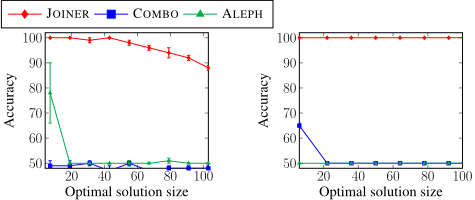
- Q3. To evaluate scalability, for increasing values of k, we generate a task where an optimal solution has size k. We learn a hypothesis with a single splittable rule. We use a zendo task similar to the one shown in Section 1 and a string task.
- Q4. We provide JOINER and COMBO with identical input. The only differences are (i) the join stage, and (ii) the elimination of splittable programs in the generate stage. However, because it can build conjunctions in the join stage, JOINER searches a larger hypothesis space than COMBO. ALEPH uses a different bias than JOINER to define the hypothesis space. In particular, ALEPH expects a maximum rule size as input. Therefore, the comparison is less fair and should be viewed as indicative only.
Experimental Results
Q1. Can the Join Stage Improve Performance?
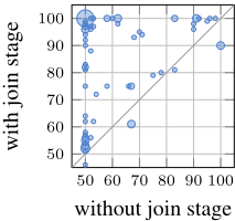
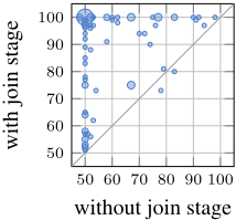
Figure 3 shows that the join stage can drastically improve predictive accuracies. AMcNeymar's test confirms (p < 0.01) that the join stage improves accuracies on 24/42 tasks with a 60s timeout and on 22/42 tasks with a 600s timeout. There is no significant difference for the other tasks.
The join stage can learn big rules which otherwise cannot be learned. For instance, for the task pharma1, the join stage finds a rule of size 17 which has 100% accuracy. By contrast, without the join stage, no solution is found, resulting in default accuracy (50%). Similarly, an optimal solution for the task iggp-rainbow has a single rule of size 19. This rule is splittable and is the conjunction of 6 small rules. The join stage identifies this rule in less than 1s as it entails all the positive examples. By contrast, without the join stage, the system exceeds the timeout without finding a solution as it needs to search through the set of all rules up to size 19 to find a solution.
The overhead of the join stage is small. For instance, for the task scale in the 1D-ARC domain, the join stage takes less than 1% of the total learning time, yet this stage allows us to find a perfectly accurate solution with a rule of size 13.
Overall, the results suggest that the answer to Q1 is that the join stage can substantially improve predictive accuracy.
Q2. Can Eliminating Splittable Programs Improve Performance?
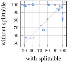
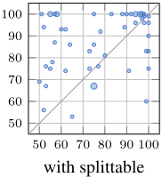
Figure 4 shows that eliminating splittable programs in the generate stage can improve learning performance. AMcNeymar's test confirms (p < 0.01) that eliminating splittable programs improves performance on 8/42 tasks with a 60s timeout and on 11/42 tasks with a 600s timeout. It degrades performance (p < 0.01) on 1/42 tasks with a 60s timeout. There is no significant difference for the other tasks.
Eliminating splittable programs from the generate stage can greatly reduce the number of programs JOINER considers. For instance, for iggp-rainbow, the hypothesis space contains 1,986,422 rules of size at most 6, but only 212,564 are nonsplittable. Likewise, for string2, when eliminating splittable programs, JOINER finds a perfectly accurate solution in 133s (2min13s). By contrast, with splittable programs, JOINER considers more programs and fails to find a solution within the 600s timeout, resulting in default accuracy (50%).
Overall, these results suggest that the answer to Q2 is that eliminating splittable programs from the generate stage can improve predictive accuracies.
without splittable
Q3. HowWell Does JOINER Scale?
Figure 5 shows that JOINER can learn an almost perfectly accurate hypothesis with up to 100 literals for both the zendo and string tasks. By contrast, COMBO and ALEPH struggle to learn hypotheses with more than 10 literals. JOINER learns a zendo hypothesis of size k after searching for programs of size 4. By contrast, COMBO must search for programs up to size k to find a solution. Similarly, an optimal solution for the string task is the conjunction of programs with 6 literals each. By contrast, COMBO must search for programs up to size k to find a solution. ALEPH struggles to learn recursive programs and thus struggles on the string task.
Overall, these results suggest that the answer to Q3 is that JOINER can scale well with the size of rules.
Q4. How Does JOINER Compare to Other Approaches?
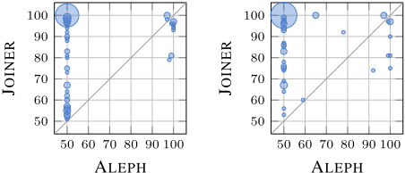
Table 1 shows the predictive accuracies aggregated over each domain. It shows JOINER achieves higher accuracies than both COMBO and ALEPH on almost all domains.
| Task | ALEPH | COMBO | JOINER |
|---|---|---|---|
| iggp zendo imdb string | 78 ± 3 | 86 ± 2 | 96 ± 1 |
| 100 ± 0 | 86 ± 3 | 94 ± 2 | |
| pharma | 50 ± 0 | 53 ± 2 | 98 ± 1 |
| 67 ± 6 | 100 ± 0 | 100 ± 0 | |
| 50 ± 0 | 50 ± 0 | 100 ± 0 | |
| onedarc | 51 ± 1 | 57 ± 2 | 89 ± 1 |
Figure 6 shows that JOINER outperforms COMBO. AMcNeymar's test confirms (p < 0.01) that JOINER outperforms COMBO on 27/42 tasks with a 60s timeout and on 26/42 tasks with a 600s timeout. JOINER and COMBO have similar performance on other tasks. JOINER can find hypotheses with big rules. For example, the flip task in the 1D-ARC domain involves reversing the order of colored pixels in an image. JOINER finds a solution with two splittable rules of size 9 and 16. By contrast, COMBO only searches programs of size at most 4 before it timeouts and it does not learn any program. JOINER can also perform better when learning non-splittable programs. For instance, JOINER learns a perfectly accurate solution for iggp-rps and proves that this solution is optimal in 20s. By contrast, COMBO requires 440s (7min20s) to find the same solution and prove optimality.
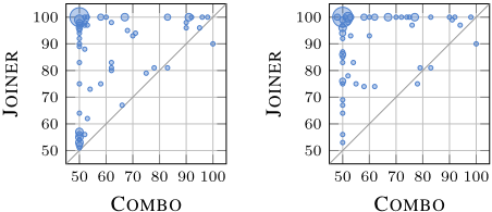
Figure 7 shows that JOINER outperforms ALEPH. A McNeymar's test confirms (p < 0.01) that JOINER outperforms ALEPH on 28/42 tasks with both 60s and 600s timeouts. ALEPH outperforms (p < 0.01) JOINER on 4/42 tasks with a 60s timeout and on 2/42 tasks with a 600s timeout. JOINER and ALEPH have similar performance on other tasks. ALEPH struggles to learn recursive programs and therefore does not perform well on the string tasks. JOINER also consistently surpasses ALEPH on tasks which do not require recursion. For instance, JOINER achieves 98% average accuracy on the pharma tasks while ALEPH has default accuracy (50%). However, for zendo3, ALEPH can achieve better accuracies (100% vs 79%) than JOINER. An optimal solution is not splittable and JOINER exceeds the timeout.
Overall, the results suggest that the answer to Q4 is that JOINER can outperform other approaches in terms of predictive accuracy.
6 Conclusions and Limitations
Learning programs with big rules is a major challenge. To address this challenge, we introduced an approach which learns big rules by joining small rules. We implemented our approach in JOINER, which can learn optimal and recursive programs. Our experiments on various domains show that JOINER can (i) learn splittable rules with more than 100 literals, and (ii) outperform existing approaches in terms of predictive accuracies.
Limitations
Splittability. Our join stage builds splittable rules. The body of a splittable rule is split into subsets which do not share bodyonly variables. Future work should generalise our approach to split rules into subsets which may share body-only variables.
Noise. In the join stage, we search for conjunctions which entail some positive examples and no negative examples. Our approach does not support noisy examples. Hocquette et al. [2024] relax the LFF definition based on the minimal description length principle. Future work should combine our approach with their approach to learn big rules from noisy data.
7 Appendices, Code, and Data
A longer version of this paper with the appendices is available at https://arxiv.org/pdf/2401.16215.pdf. The experimental code and data are available at https://github.com/ celinehocquette/ijcai24-joiner.
Acknowledgements
The first and fifth authors are supported by the EPSRC fellowship (EP/V040340/1). The second and fourth authors are supported by the Research Council of Finland (grants 347588 and 356046). The authors thank David Cerna, Filipe Gouveia, and Minghao Liu for valuable feedback. For open access, the authors have applied a CC BY public copyright licence to any author-accepted manuscript version arising from this submission.
@inproceedings{ijcai2024p380,
  title     = {Learning Big Logical Rules by Joining Small Rules},
  author    = {Hocquette, Céline and Niskanen, Andreas and Morel, Rolf and Järvisalo, Matti and Cropper, Andrew},
  booktitle = {Proceedings of the Thirty-Third International Joint Conference on
               Artificial Intelligence, {IJCAI-24}},
  publisher = {International Joint Conferences on Artificial Intelligence Organization},
  editor    = {Kate Larson},
  pages     = {3430--3438},
  year      = {2024},
  month     = {8},
  note      = {Main Track},
  doi       = {10.24963/ijcai.2024/380},
  url       = {https://doi.org/10.24963/ijcai.2024/380},
}
TY - CPAPER TI - Learning Big Logical Rules by Joining Small Rules AU - Hocquette, Céline AU - Niskanen, Andreas AU - Morel, Rolf AU - Järvisalo, Matti AU - Cropper, Andrew T2 - Proceedings of the Thirty-Third International Joint Conference on Artificial Intelligence, IJCAI-24 PB - International Joint Conferences on Artificial Intelligence Organization PY - 2024 SP - 3430 EP - 3438 DO - 10.24963/ijcai.2024/380 UR - https://doi.org/10.24963/ijcai.2024/380 ER -Copied
Machine-readable versions of this paper, for tools and AI agents:





