
Machine Unlearning via Null Space Calibration
Proceedings of the Thirty-Third International Joint Conference on Artificial Intelligence. Main Track. Pages 358-366.
https://doi.org/10.24963/ijcai.2024/40
Keywords
- AI Ethics, Trust, Fairness: ETF: Trustworthy AI
- AI Ethics, Trust, Fairness: ETF: Accountability
- AI Ethics, Trust, Fairness: ETF: Other
- AI Ethics, Trust, Fairness: ETF: Ethical, legal and societal issues
Abstract
Machine unlearning aims to enable models to forget specific data instances when receiving deletion requests. Current research centers on efficient unlearning to erase the influence of data from the model and neglects the subsequent impacts on the remaining data. Consequently, existing unlearning algorithms degrade the model's performance after unlearning, known as over-unlearning. This paper addresses this critical yet under-explored issue by introducing machine Unlearning via Null Space Calibration (UNSC), which can accurately unlearn target samples without over-unlearning. On the contrary, by calibrating the decision space during unlearning, UNSC can significantly improve the model's performance on the remaining samples. In particular, our approach hinges on confining the unlearning process to a specified null space tailored to the remaining samples, which is augmented by strategically pseudo-labeling the unlearning samples. Comparison against several established baselines affirms the superiority of our approach.
- [Allen-Zhu et al., 2019] Zeyuan Allen-Zhu, Yuanzhi Li, and Zhao Song. A convergence theory for deep learning via over-parameterization. In International conference on ma- chine learning, pages 242-252. PMLR, 2019.
- [Bourtoule et al., 2021] Lucas Bourtoule, Varun Chan- drasekaran, Christopher Choquette-Choo, Hengrui Jia, Adelin Travers, Baiwu Zhang, David Lie, and Nicolas Papernot. Machine unlearning. In Proceedings of the 42nd IEEE Symposium on Security and Privacy, 2021.
- [Cao and Yang, 2015] Yinzhi Cao and Junfeng Yang. To- wards making systems forget with machine unlearning. In 2015 IEEE symposium on security and privacy, pages 463-480. IEEE, 2015.
- [Chen et al., 2023] Min Chen, Weizhuo Gao, Gaoyang Liu, Kai Peng, and Chen Wang. Boundary unlearning: Rapid forgetting of deep networks via shifting the decision boundary. In Proceedings of the IEEE/CVF Conference on Computer Vision and Pattern Recognition (CVPR), pages 7766-7775, June 2023.
- [Fan et al., 2023] Chongyu Fan, Jiancheng Liu, Yihua Zhang, Dennis Wei, Eric Wong, and Sijia Liu. Salun: Em- powering machine unlearning via gradient-based weight saliency in both image classification and generation. arXiv preprint arXiv:2310.12508, 2023.
- [Farajtabar et al., 2020] Mehrdad Farajtabar, Navid Azizan, Alex Mott, and Ang Li. Orthogonal gradient descent for continual learning. In International Conference on Artifi- cial Intelligence and Statistics, pages 3762-3773. PMLR, 2020.
- [Ginart et al., 2019] Antonio Ginart, Melody Guan, Gregory Valiant, and James Y Zou. Making ai forget you: Data deletion in machine learning. Advances in neural infor- mation processing systems, 32, 2019.
- [Golatkar et al., 2020] Aditya Golatkar, Alessandro Achille, and Stefano Soatto. Eternal sunshine of the spotless net: Selective forgetting in deep networks. In Proceedings of the IEEE/CVF Conference on Computer Vision and Pat- tern Recognition, pages 9304-9312, 2020.
- [Graves et al., 2021] Laura Graves, Vineel Nagisetty, and Vijay Ganesh. Amnesiac machine learning. In Proceed- ings of the AAAI Conference on Artificial Intelligence, vol- ume 35, pages 11516-11524, 2021.
- [Guo et al., 2019] Chuan Guo, Tom Goldstein, Awni Han- nun, and Laurens Van Der Maaten. Certified data re- moval from machine learning models. arXiv preprint arXiv:1911.03030, 2019.
- [Gur-Ari et al., 2018] Guy Gur-Ari, Daniel A Roberts, and Ethan Dyer. Gradient descent happens in a tiny subspace. arXiv preprint arXiv:1812.04754, 2018.
- [Hayase et al., 2020] Tomohiro Hayase, Suguru Yasutomi, and Takashi Katoh. Selective forgetting of deep net- works at a finer level than samples. arXiv preprint arXiv:2012.11849, 2020.
- [He et al., 2015] Kaiming He, Xiangyu Zhang, Shaoqing Ren, and Jian Sun. Deep residual learning for image recog- nition, 2015.
- [Hoofnagle et al., 2019] Chris Jay Hoofnagle, Bart Van Der Sloot, and Frederik Zuiderveen Borgesius. The eu- ropean union general data protection regulation: what it is and what it means. Information & Communications Tech- nology Law, 28(1):65-98, 2019.
- [Hu et al., 2023] Hongsheng Hu, Shuo Wang, Jiamin Chang, Haonan Zhong, Ruoxi Sun, Shuang Hao, Haojin Zhu, and Minhui Xue. A duty to forget, a right to be assured? expos- ing vulnerabilities in machine unlearning services. arXiv preprint arXiv:2309.08230, 2023.
- [Koh and Liang, 2017] Pang Wei Koh and Percy Liang. Un- derstanding black-box predictions via influence functions. In International conference on machine learning, pages 1885-1894. PMLR, 2017.
- [Krizhevsky et al., 2009] Alex Krizhevsky, Geoffrey Hinton, et al. Learning multiple layers of features from tiny im- ages. 2009.
- [Krizhevsky et al., 2012] Alex Krizhevsky, Ilya Sutskever, and Geoffrey E Hinton. Imagenet classification with deep convolutional neural networks. Advances in neural infor- mation processing systems, 25, 2012.
- [Lee and Choi, 2018] Yoonho Lee and Seungjin Choi. Gradient-based meta-learning with learned layerwise met- ric and subspace. In International Conference on Machine Learning, pages 2927-2936. PMLR, 2018.
- [Li et al., 2018] Chunyuan Li, Heerad Farkhoor, Rosanne Liu, and Jason Yosinski. Measuring the intrinsic dimension of objective landscapes. arXiv preprint arXiv:1804.08838, 2018.
- [Li et al., 2022] Tao Li, Lei Tan, Zhehao Huang, Qinghua Tao, Yipeng Liu, and Xiaolin Huang. Low dimensional trajectory hypothesis is true: Dnns can be trained in tiny subspaces. IEEE Transactions on Pattern Analysis and Machine Intelligence, 45(3):3411-3420, 2022.
- [Li et al., 2023] Guanghao Li, Li Shen, Yan Sun, Yue Hu, Han Hu, and Dacheng Tao. Subspace based federated un- learning, 2023.
- [Lin et al., 2023] Shen Lin, Xiaoyu Zhang, Chenyang Chen, Xiaofeng Chen, and Willy Susilo. Erm-ktp: Knowledge- level machine unlearning via knowledge transfer. In Pro- ceedings of the IEEE/CVF Conference on Computer Vision and Pattern Recognition, pages 20147-20155, 2023.
- [Liu et al., 2018] Zhenhua Liu, Jizheng Xu, Xiulian Peng, and Ruiqin Xiong. Frequency-domain dynamic pruning for convolutional neural networks. Advances in neural in- formation processing systems, 31, 2018.
- [McInnes et al., 2018] Leland McInnes, John Healy, and James Melville. Umap: Uniform manifold approximation and projection for dimension reduction. arXiv preprint arXiv:1802.03426, 2018.
- [Netzer et al., 2011] Yuval Netzer, Tao Wang, Adam Coates, Alessandro Bissacco, Baolin Wu, Andrew Y Ng, et al. Reading digits in natural images with unsupervised feature learning. In NIPS workshop on deep learning and unsu- pervised feature learning, volume 2011, page 7. Granada, Spain, 2011.
- [Rosenfeld et al., 2020] Elan Rosenfeld, Ezra Winston, Pradeep Ravikumar, and Zico Kolter. Certified robust- ness to label-flipping attacks via randomized smoothing. In International Conference on Machine Learning, pages 8230-8241. PMLR, 2020.
- [Saha et al., 2021] Gobinda Saha, Isha Garg, and Kaushik Roy. Gradient projection memory for continual learning. arXiv preprint arXiv:2103.09762, 2021.
- [Shokri et al., 2017] Reza Shokri, Marco Stronati, Con- gzheng Song, and Vitaly Shmatikov. Membership infer- ence attacks against machine learning models, 2017.
- [Simonyan and Zisserman, 2015] Karen Simonyan and An- drew Zisserman. Very deep convolutional networks for large-scale image recognition, 2015.
- [Springenberg et al., 2015] Jost Tobias Springenberg, Alexey Dosovitskiy, Thomas Brox, and Martin Ried- miller. Striving for simplicity: The all convolutional net, 2015.
- [Xiao et al., 2017] Han Xiao, Kashif Rasul, and Roland Vollgraf. Fashion-mnist: a novel image dataset for bench- marking machine learning algorithms. arXiv preprint arXiv:1708.07747, 2017.
- [Xu et al., 2023] Heng Xu, Tianqing Zhu, Lefeng Zhang, Wanlei Zhou, and Philip S Yu. Machine unlearning: A survey. ACM Computing Surveys, 56(1):1-36, 2023.
References were extracted automatically from the PDF and may contain errors.
Full text extracted automatically from the PDF; figures, tables and equations may differ. The PDF is the version of record.
1 Introduction
With the rising concerns regarding the privacy of users' data in the AI era, legislative bodies have instituted regulatory measures to safeguard user's data. A notable example is the Right to Be Forgotten, which requires service providers to remove users' data from AI models upon receiving deletion requests [Hoofnagle et al., 2019]. However, removing the trace of particular data from a trained model is challenging. Machine unlearning has emerged as a promising solution. It endeavors to enable models to forget specific data samples, effectively erasing their influence as if they were never trained on these samples. The simplest way is to retrain the model from scratch without unlearning samples. However, it is timeconsuming and even impossible in the face of frequent unlearning requests. As such, the research community has been actively developing algorithms to expedite unlearning.
∗work done while at University of Queensland
† corresponding author
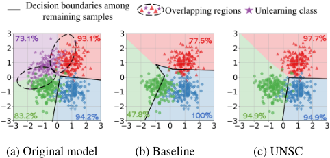
However, current unlearning methods find that the unlearning process significantly affects the remaining data, leading to over-unlearning [Hu et al., 2023; Fan et al., 2023]. The model loses part of its prediction performance on the remaining data after unlearning. This is because the unlearning process requires modifications to the weights of the original model. Though the intent was to eliminate the influence of the unlearning data, these modifications inadvertently resulted in partial forgetting of the remaining samples, ultimately leading to over-unlearning. This raises a compelling question:
Q1: To maintain the model's performance, can we prevent over-unlearning, and if so, how to achieve it?
In this paper, we propose machine Unlearning via Null Space Calibration (UNSC). To avoid over-unlearning, UNSC constrains the unlearning process within a null space tailored to the remaining samples. This ensures unlearning does not negatively impact the model's performance on the remaining samples. Figure 1c visualizes this concept, where decision boundaries among remaining samples closely resemble those depicted in Figure 1a. Going beyond, we further ask:
Q2: Is it possible to improve the model's performance after unlearning, and how?
To answer this question, we find that targeted unlearning can mitigate class overlap and augment the model's accuracy.
Therefore, calibrating the decision space might be a possible solution. Take a toy case shown in Figure 1 as an example. We train a model to classify a mixture of four Gaussian distributions. Figure 1a depicts the decision boundaries. Due to the overlap of the purple class with other classes, the model struggles to distinguish the overlapping samples. Unlearning misclassified samples and calibrating decision space lead to more accurate decision boundaries shown in Figure 1c.
UNSC assigns pseudo-labels to unlearning samples based on their proximity to the remaining samples. This process reallocates the space of unlearning samples to the remaining classes, forming more separable clusters (as shown in Figure 4d). Contributions of this paper are summarized as follows:
- We tackle the challenging problem of over-unlearning. Going beyond, we investigate the possibility of boosting the model's performance after unlearning.
- We propose UNSC, a novel machine unlearning method that confines the unlearning process to a specific null space and assigns pseudo-labels to the unlearning samples. Combined, UNSC is not only free from overunlearning but can also boost the model's performance.
- We provide theoretical justifications for the proposed method and empirically validate it with extensive experiments. The results show UNSC can provide equivalent and even better performance than retraining.
2 RelatedWorks
2.1 Machine Unlearning
Current unlearning algorithms have two branches: exact unlearning and approximate unlearning [Xu et al., 2023]. Exact unlearning ensures that distributions of model weights in an unlearned model are indistinguishable from those in a model retrained from scratch. [Cao and Yang, 2015] explore this concept within the realm of statistical query learning, [Ginart et al., 2019] propose an efficient data elimination algorithm for k-means clustering. However, these methods can not be generalized to deep learning. To address this limitation, SISA [Bourtoule et al., 2021] divides the training data into several segments and trains sub-models on each segment. It only needs to retrain the affected segment when unlearning requests arise. Nevertheless, the computational overhead of the exact unlearning method remains substantial.
Unlike exact unlearning, approximate unlearning is bounded by an approximate guarantee. Works in this stream estimate the influence of unlearning samples and modify the model weights to achieve unlearning. For example, [Graves et al., 2021] make the estimation through the gradient, [Guo et al., 2019] develop their method on the influence function [Koh and Liang, 2017]. [Golatkar et al., 2020] use the fisher information matrix in their design. [Lin et al., 2023] associate the unlearning samples with feature maps. While our work belongs to this category, it does not require the estimation of the influence of unlearning samples.
Works most closely related to ours are those by [Chen et al., 2023; Li et al., 2023]. Both [Chen et al., 2023] and our approach shift decision boundaries. The distinct advantage of our work lies in the design of a sophisticated null space, which maintains the decision boundaries of the remaining classes, leading to better performance. [Li et al., 2023] also explore subspace-based unlearning; however, their approach does not capitalize on unlearning samples to guide the shifting of decision boundaries, an essential aspect of our method.
2.2 Subspace Learning
DNNs are usually over-parameterized as they have more parameters than input samples. However, the intrinsic dimension is much smaller [Allen-Zhu et al., 2019]. The weight updates happen in a much smaller subspace than the original parameter space. [Li et al., 2018] find that optimizing in a reduced subspace reaches 90% performance of regular SGD training. [Gur-Ari et al., 2018] observe that after a short training period, the weight updates converge to a tiny subspace spanned by several top eigenvectors of the Hessian matrix.
Learning in subspace has many applications. [Li et al., 2022] optimize DNNs in a 40-dimensional subspace and achieve comparable performance to regular training over thousands or even millions of parameters. In the context of meta-learning, [Lee and Choi, 2018] employ a learned subspace within each layer's activation space where task-specific learners perform gradient descent. This subspace is tailored to be sensitive to task-specific requirements, facilitating more effective learning across different tasks. Subspace has also been applied in continual learning to mitigate catastrophic forgetting [Farajtabar et al., 2020; Saha et al., 2021].
3 Preliminaries and Notation
We use bold lowercase to denote vectors, e.g., xi, and italics in uppercase for space or set, e.g., S. The training dataset is represented as D = {xi, yi}Ni=1 ⊆ X × Y, where X ⊆ Rd is the input space and Y = {1, ..., K} is the label space. We further split D into unlearning set Du and remaining set Dr. We consider unlearning a neural network f with L layers. The input feature of input xi at layer l is denoted as ril . We denote f(·, θo) the original model trained on D with parameters θo = {w1 o , ..., wL o }, and f(·, θr) is trained on Dr.
A machine unlearning algorithm takes the original model f(·, θo) and the unlearning samples Du as input and outputs an unlearned model f(·, θu), in which the trace of the unlearning samples is removed. It can be formally defined as:
Definition 1 (Machine unlearning). [Cao and Yang, 2015] Given a model f(·, θo) = A(D) trained on dataset D with some training algorithm A, denote Du ⊆ D the set of samples that we want to remove from the training dataset D as well as from the trained model A(D). An unlearning process U produces a new set of weights θu that performs as though it had never seen the unlearning dataset Du.
UNSC constrains the unlearning process within a null space tailored to the remaining samples, which is defined as:
Definition 2 (Null space). Let A be an m by n matrix, the null space of A, denoted by null(A), is the set of all vectors
η ∈ Rn that satisfy Aη = 0.
4 ProposedMethod
Our proposed method consists of two key parts: 1) unlearning in the null space to avoid over-unlearning and 2) calibrating decision space to improve the model's performance.
4.1 Find the Null Space for Unlearning
An ideal unlearning algorithm should erase the trace about the unlearning samples from the model without degrading the model's performance on the remaining samples, i.e., without over-unlearning. To achieve this, UNSC constrains the unlearning process within a null space tailored to the remaining samples. The underlying principle is that different models with weights in the same null space would yield identical predictions on the samples associated with that null space (theoretical justification is provided in Section 5.1).
Gradients lie in the subspace spanned by inputs. Considering a single-layer neural network performing a binary classification task. The loss function is defined as:
in which σ(z) = 1 1+e-z is the sigmoid function. According to the chain rule, we have:
Substitute the last term with the derivative of the sigmoid function, we get:
ei is the prediction error. Eq. 5 shows the gradient lies in the space span{x1, x2, ..., xN}. The same relation can be deduced for the convolutional layer by reformulating the convolution into matrix multiplication [Liu et al., 2018].
Identify the layer-wise subspace for each class. Based on the relationship between gradient and inputs, we first identify the subspace of each class. Then, for each unlearning sample, we find the corresponding null space to perform unlearning. This incurs negligible computation overhead. For each class, we only need a small batch of samples (256 in our experiment) to find the null space. In addition, we only need to find the subspace once because we treat the null space as fixed during unlearning. Our experiment results justify the hypothesis. One may consider iterative updating the null space during unlearning. We leave this as future work.
To find the subspace of class k, we sample a batch of inputs Bk = {(xi, yi)|yi = k}Bi=1 from class k at random and feed these samples through the original model f(·; θo). At the l-th layer, we have a collection of input features as Rkl = [rl,1, rl,2, ..., rl,B] with each column corresponds to an input. For the convolutional layer, we need to reformulate the input feature by treating each patch as a column. The columns of Rcl are usually larger than the rows, and each column represents a vector sampled from some unknown subspace. We Algorithm 1 Find layer-wise subspace of class k
Input: Batch input {xi, yi|yi = k}Bi=1 ; network f(·; θo); threshold {ϵl}Ll=1 .
Output: Layer-wise subspace of class k.
- 1: Feed forward {xi}Bi=1 through f(·; θo).
- 2: for l ∈ [L] do
- 3: Collect the input feature Rkl .
- 4: Perform SVD: Rl =Ukl Σkl VkT l .
- 5: end for
- 6: return S k = {Ukl }Ll=1 .
decompose it using singular value decomposition (SVD) to find the subspace as:
The elements in Ukl are the subspace basis for class k at layer l. The gradient induced by samples from class k lies in this subspace. Σkl is a diagonal matrix that stores the eigenvalues in descending order. We repeat this process of all layers in f(·; θo) to identify subspaces of each layer,
Algorithm 1 formalizes this process. Note that the inputs do not need to be from the same class. However, in our design, we find the layer-wise subspace S k of each class for efficient unlearning. The unlearning samples could come from different classes. For each unlearning sample, we need to find the corresponding null space to perform unlearning. By identifying class-wise null space, we can efficiently identify each unlearning sample's null space. We articulate this in the following part.
Unlearning in the null space. After getting the layer-wise subspaces of each class, we are ready to find the null space for unlearning. For an unlearning sample (xi, yi = c) ∈ Du, we perform unlearning in the null space of the rest classes ¯ c = {i ∈ [K]|i ̸= c}. Denote the concatenation of the rest subspaces as S ¯ c l = ∪i∈¯ cUil at layer-l. We merge these subspaces as:
The basis of the merged subspace comes from the element of U¯ cl . S ¯ c l has few dominant eigenvalues and a large number of very small ones. The eigenvectors corresponding to those small eigenvalues are usually irrelevant. Thus, we can approximate the subspace by the span of top-k eigenvectors.
where ϵl is the approximation threshold (we find ϵl > 0.97 is good enough in our experiment), ∥A∥F is Frobenius norm of matrix A. The top-k eigenvectors span the approximate subspace:
where u¯ cl,i is the i-th element of U¯ cl . Gradient lies in ˆS¯ cl will alter the model's response to samples from ¯ c, which may lead to over-unlearning. As such, we project the gradient to a space perpendicular to ˆS¯ cl , i.e., the null space of the rest samples. The projection matrix is defined as:
At layer-l, the updating rule is modified as:
where Lc is the classification loss on unlearning sample (xi, yi = c). Algorithm 2 illustrates the pseudo-code.
4.2 Calibrate Decision Space
To calibrate the decision space, we borrow the idea from poisoning attacks, which aim to decrease the victim model's performance by feeding it poisoned samples. There are several poisoning attacks, one of which is the label-flipping attack [Rosenfeld et al., 2020]. In this attack, the input feature xi remains unchanged, and the label is carefully set as the most dissimilar class. But our target is different, i.e., we aim to boost the model's utility on the remaining samples. As such, we label an unlearning sample as the most similar class in the rest of the classes.
However, comparing samples-wise similarity could be rather inefficient and even impossible when the remaining samples are not accessible. As such, we base our method on the prediction of the original model. For an unlearning sample of class (xi, yi = c), we find the pseudo-labels from the remaining classes set ¯ c as:
We use the top-1 prediction as the pseudo-label for an unlearning sample if it gives the wrong prediction. Otherwise, we use the second-highest score as the pseudo-label.
To elucidate our design, one might consider this in another way: we expect the unlearned model to behave similarly to the retrained model. The unlearned model should give the same or similar predictions as the retrained model for the unlearning samples. The retrained model, trained using the remaining samples, has never been exposed to the unlearning samples. Consequently, the retrained model will classify these unlearning samples into categories represented within the remaining samples. As such, the unlearned model should predict a given unlearning sample belongs to the same class as the remaining samples most similar to it.
5 Theoretical Analysis
5.1 Null Space Prevents Over-unlearning
Theorem 1. For a trained model f(·; θo), unlearning the target samples fromDu in the null space tailored to the remaining samples from Dr ensures the unlearned model f(·; θu) has approximately the same performance as f(·; θo), i.e.,
where Lr(θ) := 1 |Dr | ∑Dr ℓ(f(xi; θ), yi) is the average loss on the remaining samples.
Algorithm 2 Unlearning via null space calibration
Input: Training data D; trained model f(·; θo).
- Output: Unlearned model f(·; θu) 1: # Get the subspace of each class 2: for k ∈ [K] do 3: Identify the subspace of class k by Algorithm 1 with {xi, yi|yi = k}Bi=1 , f(·; θo), and {ϵl}Ll=1 as input. 4: end for 5: # Calculate the projection matrix 6: for c ∈ [K] do 7: for l ∈ [L] do 8: Merge subspaces of rest classes using Eq. 8. 9: Perform k-rank approximation by Eq. 9 10: Find the subspace as Eq. 10. 11: Calculate layer-wise projection matrix as Eq. 11. 12: end for 13: end for 14: # Unlearning in the null space 15: for (xi, yi) ∈ Du do 16: ˜ yi ← arg maxy∈¯ c f(xi; θo) ▷ Pseudo-labeling xi 17: Calculate gradients on (xi, ˜ yi). 18: Update the original model in the null space as Eq. 12.
- 19: end for
Proof. We expand Lr(θu) around Lr(θo) as:
We decompose ∆θT ∇θLr(θo) layer-by-layer as:
Note θ = {w1 , ...,wL} and ∆wl = w1u - w1 o . At the lth layer, we have rl+1 i = σ(wl rli ), where σ(·) is activation function, rli is the activation at layer l with respect to input xi. We rewrite the derivative term by the chain rule:
Note that we confine the learning in a null space tailored to the reaming samples fromDr. Thus, at the l-th layer, we have the following by definition:
Thus, we immediately have ∆θT ∇θLr(θo) = 0. During unlearning, ∆θ should be relatively small. As such, we have:
Theorem 1 asserts that confining unlearning in the null space ensures the unlearned model f(·, θu) performs comparably to the original model f(·, θo). This substantiates that UNSC can effectively mitigate the risk of over-unlearning.
5.2 Pseudo-labeling Benefits Unlearning
Assuming the unlearning sample xi is generated i.i.d. from the domain ⟨Du, ho⟩, with the ground-truth labeling function ho. In our proposed method, we assign pseudo-labels to the unlearning samples, this equivalent to replacing ho with a new labeling function hu. Consequently, the domain of unlearning samples becomes ⟨Du, hu⟩ during learning. The primary objective of unlearning is to minimize the model's retention of information about the unlearning samples. We use the empirical risk of unlearning samples as a proxy measurement of forgetting in our analysis. The risk of f(·; θu) over ⟨Du, hu⟩ is calculated as:
We use the parallel notion ϵu(θu, ho) to denote the risk over the original domain ⟨Du, ho⟩, which can be expressed as:
The forgetting level ϵ(θu, h0) depends partly on the second term on the right-hand side. It measures the expectation that the pseudo-labeling function disagrees with the ground-truth labeling function for the unlearning samples. To facilitate forgetting, hu should assign each unlearning sample a label different from ho(xi) to minimize Exi∈Du [1ho(xi)=hu(xi)]. The pseudo-label assigned by UNSC differs from the groundtruth label ho(xi). Thus, it minimizes the second term and increases ϵ(θu, ho), leading to better forgetting.
6 Experiments
6.1 Protocol and EvaluationMetrics
Datasets and models. We compare UNSC with existing methods on the standard FashionMNIST [Xiao et al., 2017], CIFAR-10, CIFAR-100 [Krizhevsky et al., 2009], and SVHN [Netzer et al., 2011] benchmarks. We use AlexNet [Krizhevsky et al., 2012] for FashionMNIST, VGG-11 [Simonyan and Zisserman, 2015] for SVHN, AllCNN [Springenberg et al., 2015] for CIFAR-10, and ResNet-18 [He et al., 2015] for CIFAR-100.
Evaluation metrics. We evaluate the unlearning process from two aspects, i.e., utility and privacy guarantee. (1) Utility guarantee is evaluated by accuracy on the remaining testing data AccDrt and accuracy on the unlearning testing data AccDut . An ideal unlearning process should sustain AccDrt and reduce AccDrt towards zero [Chen et al., 2023]. (2) Privacy guarantee is assessed through the membership inference attack (MIA) [Shokri et al., 2017]. Following [Fan et al., 2023], we apply the confidence-based MIA predictor to the unlearned model on the unlearning samples. We define the MIA accuracy as the True Negative Rate AccMIA = TN/|Du|, i.e., the rate of unlearning samples that are identified as not being in the training set of the unlearned model. A higher AccMIA indicates a more effective unlearning. All results are averaged over three trials by default 1 .
1 Code released at https://github.com/HQC-ML/UNSC
Implementation details. The training set is divided into 90% for training and 10% for validation. We train the original and retrained models for 200 epochs and stop the training based on validation accuracy. The patience is set to 30. We use SGD optimizer in all experiments, starting with a learning rate of 0.1, and reducing it by 0.2 at epochs 60, 120, and 160. In the unlearning stage, we determine the best learning rate and number of epochs for different datasets and networks.
6.2 Comparison with the State-of-the-Art
We compare UNSC with various methods, assessing both utility and privacy guarantees. These include: (1) Retrain, (2) Boundary unlearning (BU) [Chen et al., 2023], (3) Random labels (RL) [Hayase et al., 2020], (4) Gradient ascent (GA) [Golatkar et al., 2020], (5) Fisher Forgetting (Fisher) [Golatkar et al., 2020], and (6) SalUn [Fan et al., 2023]. Following [Chen et al., 2023], we randomly select one class (or ten classes on CIFAR-100) and unlearn all the samples.
Utility guarantee. Table 1 displays the accuracy results of models obtained by different unlearning methods. Observing the results reveals that: (1) Comparison methods struggle with over-unlearning: AccDut decreases at the cost of AccDrt , leading to over-unlearning. For instance, SalUn reduces AccDut to 3.56% with a 16.7% reduction in AccDrt on the SVHN dataset. This is more sever on the CIFAR-100 dataset, as comparison methods degrade AccDrt by more than 30%; (2) UNSC excels in avoiding over-unlearning: UNSC consistently maintains AccDut below 2% without compromising AccDrt . This underscores UNSC's ability to avoid over-unlearning; (3) UNSC exhibits superior performance compared to the original model: On all datasets, models derived fromUNSCget higher AccDrt than the original models. We attribute the improvement to the calibration of decision space, which makes the remaining samples more separable.
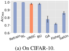
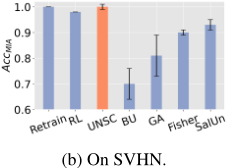
Privacy guarantee. Figure 2 depicts MIA results. By randomly selecting one class to unlearn, we get various unlearned models through different methods. We then assess these models using MIA. The retrained model, having no exposure to unlearning samples, obtains an attack accuracy of 1.0. On CIFAR-10, Fisher and GA exhibit an accuracy below 0.8, pointing to inadequate unlearning. SalUn achieves a higher accuracy but suffers more severe over-unlearning than Fisher, as evident by AccDrt in Table 1. The attack accuracy of BU and UNSC is around 0.98, signifying success unlearning. However, unlike BU, UNSC is free of over-unlearning. For SVHN, the attack accuracy of BU and GA falls below 0.8, suggesting unsuccessful unlearning. Conversely, UNSC gets an attack accuracy of 1.0.
6.3 Ablation Studies
Pseudo-labeling strategy. To demonstrate the efficacy of the proposed pseudo-labeling strategy, we conduct a thorough examination of different datasets. We present results obtained on CIFAR-10 in Figure 3a. We unlearn all samples of class 3 and assign pseudo-labels as described in Section. 4.2. Figure 3a plots distributions of pseudo-labels and labels predicted by the retrained model. The distribution of pseudo-labels aligns well with the predictions of the retrained model on unlearning samples. The consistency substantiates the effectiveness of the proposed pseudo-labeling strategy.
| Approach | FashionMNIST | SVHN | CIFAR-10 | CIFAR-100 | ||||
|---|---|---|---|---|---|---|---|---|
| AccDrt (↑) | AccDut (↓) | AccDrt (↑) | AccDut (↓) | AccDrt (↑) | AccDut (↓) | AccDrt (↑) | AccDut (↓) | |
| Original RL BU GA Fisher SalUn UNSC | 93.58±0.28 91.50±0.20 72.71±0.44 80.94±3.87 95.11±0.17 91.11±0.32 95.23±0.27 | 80.97±1.44 3.37±1.44 2.97±1.28 6.40±2.90 1.50±1.27 1.80±1.44 0.67±0.17 | 95.52±0.12 75.87±8.67 80.99±4.01 75.11±6.76 95.72±0.30 78.81±4.85 95.74±0.17 | 91.30±0.30 1.17±0.16 4.03±1.87 3.10±3.90 2.53±0.91 3.56±0.56 0.00±0.00 | 92.10±0.29 82.88±2.62 87.24±2.43 88.53±1.11 92.54±0.79 88.88±0.19 92.77±0.08 | 79.93±1.72 3.30±0.83 1.47±0.17 6.80±1.93 0.07±0.05 6.17±0.83 0.70±0.08 | 75.36±0.34 24.58±2.01 36.81±3.05 36.55±12.85 49.23±2.02 41.85±3.56 76.16±0.35 | 72.07±1.18 1.13±0.61 12.13±2.40 12.87±7.61 0.00±0.00 5.97±1.39 1.80±0.16 |
| Retrain | 95.19±0.20 | 0.00±0.00 | 95.56±0.23 | 0.00±0.00 | 93.22±0.18 | 0.00±0.00 | 75.77±0.22 | 0.00±0.00 |
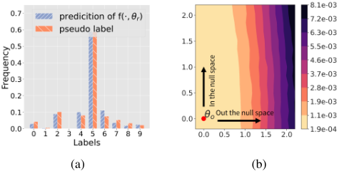
Impact of null space. Our first contribution is confining the unlearning process in a null space, which avoids overunlearning. Here, we provide experimental validation. We randomly select one class as the unlearning class and identify the corresponding null space following the steps outlined in Algorithm 1. We modify the model's weights by adding vectors composed of two components: one within the null space and one outside. We evaluate the modified model on the testing set of remaining samples and plot the loss contour in Figure 3b, with the axes displaying the scaled coefficients.
From Figure 3b, we observe that modifying weights outside the null space increases the loss, while alterations within the null space leave the loss unchanged. This pattern validates our analysis: unlearning within the null space does not impact the model's performance on the remaining samples.
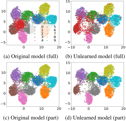
Decision space calibration. Our second contribution is the calibration of the decision space, which improves the model's performance. To illustrate this, we compare decision spaces of the original and unlearned model in Figure 4. We unlearn class 3 and visualize the latent spaces using UMAP [McInnes et al., 2018]. Several observations can be made: (1) UNSC successfully unlearns class 3 from the original model. In Figure 4b, the cluster of class 3 disperses, with its samples overlapping with adjacent samples. A clear signal that the unlearned model forgets the unlearned samples; (2) Decision boundaries among the remaining samples remain unaffected after unlearning. The shape and positions of clusters in Figure 4d closely resemble those in Figure 4c, underscoring the efficacy of UNSC in overcoming over-unlearning; (3) Better separability after unlearning. UNSC redistributes the region previously dominated by class 3 among neighboring classes, improving their separability as depicted in Figures 4c and 4d.
| #Classes | Original | Retrain | UNSC | Accuracy Gain ∆AccDrt (↑) | |||
|---|---|---|---|---|---|---|---|
| AccDrt | AccDut | AccDrt (↑) | AccDut (↓) | AccDrt (↑) | AccDut (↓) | ||
| 1 2 3 4 | 92.10±0.29 | 79.93±1.72 | 93.22±0.18 93.18±0.15 | 0.00±0.00 | 92.77±0.25 | 0.70±0.08 | 0.67±0.42 |
| 91.66±0.36 | 87.77±0.89 | 0.00±0.00 | 92.73±0.25 | 0.60±0.33 | 1.07±0.35 | ||
| 92.35±0.35 | 87.44±0.64 | 94.24±0.17 | 0.00±0.00 | 93.84±0.33 | 0.89±0.45 | 1.49±0.57 | |
| 92.38±0.36 | 88.63±0.77 | 94.28±0.36 | 0.00±0.00 | 94.08±0.21 | 0.31±0.23 | 1.70±0.54 | |
| 5 | 93.23±0.34 | 88.53±0.55 | 96.12±0.22 | 0.00±0.00 | 96.15±0.13 | 0.68±0.52 | 2.92±0.42 |
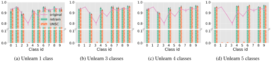
UNSC under different settings. We randomly select 1 to 5 classes to unlearn. Table 2 compares the utility guarantee of the original model, the retrained model, and the model obtained by UNSC on the CIFAR-10 dataset. Figure 5 provides a detailed class-wise accuracy breakdown.
Across different settings, the model obtained by UNSC gets near-zero accuracy on the unlearned classes. Meanwhile, the accuracy of the remaining classes is higher than that of the original model (measured by ∆AccDrt ). Furthermore, as the number of unlearned classes increases, so does the accuracy gain. This observation affirms (1) the effectiveness of null space in preventing over-unlearning and (2) the benefit of decision space calibration. As we progressively unlearn additional samples, we allocate more decision spaces to the remaining samples. This process results in a more distinguishable decision space, ultimately enhancing the model's classification performance on the remaining samples.
UNSC vs. Baselines. To discern the contribution of each component in the proposed method, we contrast UNSC with three baselines: the original model, Retrain, and RL. Table 3 presents a detailed breakdown of the results on the FashionMNIST dataset, with indexed experiments for reference.
Contribution of null space. We conduct an ablation study by removing the constraint of null space and then compare the outcomes of experiments III and IV. In the absence of null space constraints, RL reduces AccDut to 0.90%, incurring a 7.28% reduction in AccDrt . RL successfully completes the unlearning task but at the cost of excessive impact on the remaining samples. In contrast, when confining the unlearning process within a null space tailored to the remaining samples in experiment IV, we decrease AccDut to 1.57% without affecting AccDrt . This comparison highlights the effectiveness of the null space in preventing over-unlearning.
| Exp. ID | OR | RE | RL | NS | PL | AccDrt | AccDut |
|---|---|---|---|---|---|---|---|
| I II III | ✓ | ✓ | ✓ | 93.58±0.28 95.19±0.20 86.30±0.85 | 80.97±1.44 0.00±0.00 0.90±0.21 | ||
| IV V | ✓ | ✓ ✓ | ✓ | 93.30±1.12 95.23±0.27 | 1.57±0.53 0.67±0.17 |
Contribution of pseudo-labeling. We further demonstrate the benefits introduced by pseudo-labeling. Compared to experiment IV, replacing RL with pseudo-labeling increases AccDrt by 1.93% in experiment V. Thanks to pseudolabeling, the decision space of the unlearning samples can be selectively redistributed to the adjacent classes, forming a more distinguishable decision space. The combination of null space and pseudo-labeling contributes to an elevated AccDrt of 95.23%, surpassing the original model by 1.61% and even outperforming the retrained model.
7 Conclusion
This paper introduces UNSC, an accurate unlearning algorithm that addresses the challenge of over-unlearning and further enhances the model's performance after unlearning. The innovation in UNSC is grounded in two pivotal design aspects: (1) Constraining the unlearning process within a designated null space to prevent over-unlearning and (2) Pseudo-labeling the unlearning samples to calibrate the decision space, thereby improving prediction accuracy. Our theoretical analysis and empirical results convincingly demonstrate the superior performance of UNSC over baselines.
Acknowledgments
This work was supported by the Australian Research Council (ARC), Australia, through the ARC Discovery Project under Grant DP230100246 and DP240100955.
@inproceedings{ijcai2024p40,
  title     = {Machine Unlearning via Null Space Calibration},
  author    = {Chen, Huiqiang and Zhu, Tianqing and Yu, Xin and Zhou, Wanlei},
  booktitle = {Proceedings of the Thirty-Third International Joint Conference on
               Artificial Intelligence, {IJCAI-24}},
  publisher = {International Joint Conferences on Artificial Intelligence Organization},
  editor    = {Kate Larson},
  pages     = {358--366},
  year      = {2024},
  month     = {8},
  note      = {Main Track},
  doi       = {10.24963/ijcai.2024/40},
  url       = {https://doi.org/10.24963/ijcai.2024/40},
}
TY - CPAPER TI - Machine Unlearning via Null Space Calibration AU - Chen, Huiqiang AU - Zhu, Tianqing AU - Yu, Xin AU - Zhou, Wanlei T2 - Proceedings of the Thirty-Third International Joint Conference on Artificial Intelligence, IJCAI-24 PB - International Joint Conferences on Artificial Intelligence Organization PY - 2024 SP - 358 EP - 366 DO - 10.24963/ijcai.2024/40 UR - https://doi.org/10.24963/ijcai.2024/40 ER -Copied
Machine-readable versions of this paper, for tools and AI agents:





