
Fine-tuning Pre-trained Models for Robustness under Noisy Labels
Proceedings of the Thirty-Third International Joint Conference on Artificial Intelligence. Main Track. Pages 3643-3651.
https://doi.org/10.24963/ijcai.2024/403
Keywords
- Machine Learning: ML: Robustness
- Machine Learning: ML: Trustworthy machine learning
- AI Ethics, Trust, Fairness: ETF: Safety and robustness
Abstract
The presence of noisy labels in a training dataset can significantly impact the performance of machine learning models. In response to this issue, researchers have focused on identifying clean samples and reducing the influence of noisy labels. Recent works in this field have achieved notable success in terms of generalizability, albeit at the expense of extensive computing resources. Therefore, reducing computational costs remains a crucial challenge. Concurrently, in other research areas, there has been a focus on developing fine-tuning techniques to efficiently achieve high generalization performance. Despite their proven efficiently achievable generalization capabilities, these techniques have seen limited exploration from a label noise point of view. In this research, we aim to find an effective approach to fine-tune pre-trained models for noisy labeled datasets. To achieve this goal, we empirically investigate the characteristics of pre-trained models on noisy labels and propose an algorithm, named TURN. We present the results of extensive testing and demonstrate both efficient and improved denoising performance on various benchmarks, surpassing previous methods.
- Architecture
- Clothing1M LP FFT LP+FFT GCE DivideMix UNICON GCE ELR Ours ViT-B/16 67.83 / 67.54 67.46 / 67.46 66.91 / 66.91 68.13 / 68.13 68.42 / 68.42 68.98 / 68.98 69.74 / 69.74 68.73 / 68.73 70.28 / 70.28 ConvNeXt-T 64.82 / 64.81 64.59 / 64.59 64.17 / 64.17 66.12 / 65.42 67.33 / 66.92 68.80 / 68.80 68.92 / 68.92 69.19 / 68.52 69.63 / 69.63
- MAE-ViT-B 5.06 / 5.06 5.92 / 5.92 8.28 / 8.28 8.04 / 8.04 8.52 / 8.52 61.31 / 61.31 60.80 / 60.80 61.51 / 61.51 61.96 / 61.96 MSN-ViT-B 6.77 / 6.77 6.20 / 6.20 7.64 / 7.64 6.42 / 6.42 6.31 / 6.31 66.88 / 63.38 67.06 / 65.41 66.32 / 66.32 69.13 / 69.13 ResNet-50 7.08 / 7.08 7.18 / 7.18 6.68 / 6.68 8.13 / 8.13 8.24 / 8.24 66.10 / 66.02 66.19 / 66.19 66.19 / 66.19 66.31 / 66.31
- Architecture WebVision LP FFT LP+FFT CE GCE ELR DivideMix UNICON CE GCE ELR Ours ViT-B/16 84.62 / 84.48 84.32 / 84.24 84.48 / 84.32 84.72 / 84.72 85.68 / 85.68 84.20 / 83.04 83.40 / 83.40 84.92 / 83.72 85.96 / 85.92 ConvNeXt-T 85.24 / 85.24 85.12 / 85.04 86.28 / 86.28 86.40 / 86.40 86.24 / 86.24 84.00 / 82.68 85.40 / 84.92 84.52 / 83.44 87.16 / 86.44
- MAE-ViT-B 48.00 / 48.00 47.32 / 47.28 49.76 / 49.76 59.40 / 58.44 56.96 / 53.80 67.48 / 65.64 63.16 / 62.84 67.80 / 67.80 69.45 / 68.45 MSN-ViT-B 77.40 / 77.40 74.40 / 74.40 74.00 / 74.00 76.56 / 76.40 77.72 / 77.34 77.04 / 77.80 72.28 / 72.28 74.88 / 72.28 78.36 / 75.40 ResNet-50 84.88 / 84.72 81.68 / 81.68 84.96 / 84.96 85.16 / 85.16 85.04 / 85.04 78.00 / 76.44 77.04 / 70.92 80.44 / 77.44 85.36 / 85.36
- [Ahn and Yun, 2023] Sumyeong Ahn and Se-Young Yun. De- noising after entropy-based debiasing a robust training method for dataset bias with noisy labels. In Proceedings of the AAAI Conference on Artificial Intelligence, volume 37, pages 169-177, 2023.
- [Assran et al., 2022] Mahmoud Assran, Mathilde Caron, Is- han Misra, Piotr Bojanowski, Florian Bordes, Pascal Vin- cent, Armand Joulin, Mike Rabbat, and Nicolas Ballas. Masked siamese networks for label-efficient learning. In European Conference on Computer Vision, pages 456-473. Springer, 2022.
- [Baevski et al., 2022] Alexei Baevski, Wei-Ning Hsu, Qiantong Xu, Arun Babu, Jiatao Gu, and Michael Auli. Data2vec: A general framework for self-supervised learning in speech, vision and language. arXiv preprint arXiv:2202.03555, 2022.
- [Chen et al., 2020] Ting Chen, Simon Kornblith, Mohammad Norouzi, and Geoffrey Hinton. A simple framework for contrastive learning of visual representations. In Interna- tional conference on machine learning, pages 1597-1607.
- PMLR, 2020.
- [Cheng et al., 2021] Hao Cheng, Zhaowei Zhu, Xingyu Li, Yifei Gong, Xing Sun, and Yang Liu. Learning with instance-dependent label noise: A sample sieve approach. In International Conference on Learning Representations, 2021.
- [Cheng et al., 2023] Hao Cheng, Zhaowei Zhu, Xing Sun, and Yang Liu. Mitigating memorization of noisy labels via regularization between representations. In The Eleventh In- ternational Conference on Learning Representations, 2023.
- [Dosovitskiy et al., 2021] Alexey Dosovitskiy, Lucas Beyer, Alexander Kolesnikov, Dirk Weissenborn, Xiaohua Zhai, Thomas Unterthiner, Mostafa Dehghani, Matthias Min- derer, Georg Heigold, Sylvain Gelly, Jakob Uszkoreit, and Neil Houlsby. An image is worth 16x16 words: Trans- formers for image recognition at scale. In International Conference on Learning Representations, 2021.
- [He et al., 2016] Kaiming He, Xiangyu Zhang, Shaoqing Ren, and Jian Sun. Deep residual learning for image recog- nition. In Proceedings of the IEEE conference on computer vision and pattern recognition, pages 770-778, 2016.
- [He et al., 2022] Kaiming He, Xinlei Chen, Saining Xie, Yanghao Li, Piotr Dollár, and Ross Girshick. Masked au- toencoders are scalable vision learners. In Proceedings of the IEEE/CVF Conference on Computer Vision and Pattern Recognition, pages 16000-16009, 2022.
- [Huang et al., 2023] Zhizhong Huang, Junping Zhang, and Hongming Shan. Twin contrastive learning with noisy labels. In Proceedings of the IEEE/CVF Conference on Computer Vision and Pattern Recognition, pages 11661- 11670, 2023.
- [Karim et al., 2022] Nazmul Karim, Mamshad Nayeem Rizve, Nazanin Rahnavard, Ajmal Mian, and Mubarak Shah. Unicon: Combating label noise through uniform selection and contrastive learning. In Proceedings of the IEEE/CVF Conference on Computer Vision and Pattern Recognition, pages 9676-9686, 2022.
- [Kim et al., 2021] Taehyeon Kim, Jongwoo Ko, JinHwan Choi, Se-Young Yun, et al. Fine samples for learning with noisy labels. Advances in Neural Information Processing Systems, 34:24137-24149, 2021.
- [Ko et al., 2022] Jongwoo Ko, Bongsoo Yi, and Se-Young Yun. Alasca: Rethinking label smoothing for deep learning under label noise. arXiv preprint arXiv:2206.07277, 2022.
- [Ko et al., 2023] Jongwoo Ko, Sumyeong Ahn, and Se- Young Yun. EFFICIENT UTILIZATION OF PRE- TRAINED MODEL FOR LEARNING WITH NOISY LA- BELS. In ICLR 2023 Workshop on Pitfalls of limited data and computation for Trustworthy ML, 2023.
- [Krizhevsky et al., 2009] Alex Krizhevsky, Geoffrey Hinton, et al. Learning multiple layers of features from tiny images. 2009.
- [Kumar et al., 2022] Ananya Kumar, Aditi Raghunathan, Robbie Jones, Tengyu Ma, and Percy Liang. Fine-tuning can distort pretrained features and underperform out-of- distribution. arXiv preprint arXiv:2202.10054, 2022.
- [Li et al., 2017] Wen Li, Limin Wang, Wei Li, Eirikur Agusts- son, and Luc Van Gool. Webvision database: Visual learn- ing and understanding from web data. arXiv preprint arXiv:1708.02862, 2017.
- [Li et al., 2020] Junnan Li, Richard Socher, and Steven CH Hoi. Dividemix: Learning with noisy labels as semi- supervised learning. arXiv preprint arXiv:2002.07394, 2020.
- [Li et al., 2022] Shikun Li, Xiaobo Xia, Shiming Ge, and Tongliang Liu. Selective-supervised contrastive learning with noisy labels. In Proceedings of the IEEE/CVF Confer- ence on Computer Vision and Pattern Recognition, pages 316-325, 2022.
- [Liaw et al., 2018] Richard Liaw, Eric Liang, Robert Nishi- hara, Philipp Moritz, Joseph E Gonzalez, and Ion Stoica. Tune: A research platform for distributed model selection and training. arXiv preprint arXiv:1807.05118, 2018.
- [Liu et al., 2020] Sheng Liu, Jonathan Niles-Weed, Narges Razavian, and Carlos Fernandez-Granda. Early-learning regularization prevents memorization of noisy labels. Ad- vances in neural information processing systems, 33:20331- 20342, 2020.
- [Liu et al., 2021] Ze Liu, Yutong Lin, Yue Cao, Han Hu, Yix- uan Wei, Zheng Zhang, Stephen Lin, and Baining Guo. Swin transformer: Hierarchical vision transformer using shifted windows. In Proceedings of the IEEE/CVF Inter- national Conference on Computer Vision, pages 10012- 10022, 2021.
- [Liu et al., 2022] Zhuang Liu, Hanzi Mao, Chao-Yuan Wu, Christoph Feichtenhofer, Trevor Darrell, and Saining Xie. A convnet for the 2020s. In Proceedings of the IEEE/CVF Conference on Computer Vision and Pattern Recognition, pages 11976-11986, 2022.
- [Radford et al., 2021] Alec Radford, Jong Wook Kim, Chris Hallacy, Aditya Ramesh, Gabriel Goh, Sandhini Agarwal, Girish Sastry, Amanda Askell, Pamela Mishkin, Jack Clark, et al. Learning transferable visual models from natural lan- guage supervision. In International Conference on Machine Learning, pages 8748-8763. PMLR, 2021.
- [Song et al., 2022] Hwanjun Song, Minseok Kim, Dongmin Park, Yooju Shin, and Jae-Gil Lee. Learning from noisy labels with deep neural networks: A survey. IEEE Transac- tions on Neural Networks and Learning Systems, 2022.
- [Tu et al., 2023] Yuanpeng Tu, Boshen Zhang, Yuxi Li, Liang Liu, Jian Li, Yabiao Wang, Chengjie Wang, and Cai Rong Zhao. Learning from noisy labels with decoupled meta label purifier. In Proceedings of the IEEE/CVF Conference on Computer Vision and Pattern Recognition, pages 19934- 19943, 2023.
- [Van der Maaten and Hinton, 2008] Laurens Van der Maaten and Geoffrey Hinton. Visualizing data using t-sne. Journal of machine learning research, 9(11), 2008.
- [Wang et al., 2019] Yisen Wang, Xingjun Ma, Zaiyi Chen, Yuan Luo, Jinfeng Yi, and James Bailey. Symmetric cross entropy for robust learning with noisy labels. In Proceed- ings of the IEEE/CVF International Conference on Com- puter Vision, pages 322-330, 2019.
- [Xia et al., 2022] Xiaobo Xia, Tongliang Liu, Bo Han, Ming- ming Gong, Jun Yu, Gang Niu, and Masashi Sugiyama. Sample selection with uncertainty of losses for learning with noisy labels. In International Conference on Learning Representations, 2022.
- [Xiao et al., 2015] Tong Xiao, Tian Xia, Yi Yang, Chang Huang, and Xiaogang Wang. Learning from massive noisy labeled data for image classification. In Proceedings of the IEEE conference on computer vision and pattern recogni- tion, pages 2691-2699, 2015.
- [Zhang and Sabuncu, 2018] Zhilu Zhang and Mert Sabuncu. Generalized cross entropy loss for training deep neural networks with noisy labels. Advances in neural information processing systems, 31, 2018.
- [Zhang et al., 2020] Yuhao Zhang, Hang Jiang, Yasuhide Miura, Christopher D Manning, and Curtis P Langlotz. Contrastive learning of medical visual representations from paired images and text. arXiv preprint arXiv:2010.00747, 2020.
- [Zheltonozhskii et al., 2022] Evgenii Zheltonozhskii, Chaim Baskin, Avi Mendelson, Alex M Bronstein, and Or Litany. Contrast to divide: Self-supervised pre-training for learning with noisy labels. In Proceedings of the IEEE/CVF Winter Conference on Applications of Computer Vision, pages 1657-1667, 2022.
- [Zhou et al., 2021] Xiong Zhou, Xianming Liu, Junjun Jiang, Xin Gao, and Xiangyang Ji. Asymmetric loss functions for learning with noisy labels. In International conference on machine learning, pages 12846-12856. PMLR, 2021.
References were extracted automatically from the PDF and may contain errors.
Full text extracted automatically from the PDF; figures, tables and equations may differ. The PDF is the version of record.
1 Introduction
Despite the remarkable performance of deep neural networks (DNNs), their effectiveness decreases significantly when trained with inaccurate supervision. Additionally, manually correcting noisy labels or acquiring clean labels anew is challenging due to the large-scale nature of datasets. To address this issue, researchers have developed various approaches within the field of Learning with Noisy Labels (LNL). These approaches encompass robust training loss [Zhang and Sabuncu, 2018; Wang et al., 2019], regularization [Cheng et al., 2023; Ko et al., 2022], and semi-supervised learning methods [Li et al., 2020; Liu et al., 2020].
However, recent studies in the field of LNL have shown an increase in computational complexity. As demonstrated in Table 1, one of the notable algorithms called UNICON [Karim et al., 2022] incurs a substantial training time increase of 622% compared to the vanilla approach. This is primarily due to the utilization of noisy labeled samples. Notably, the most computationally expensive aspect is the careful detection and integration of noisy labeled samples. For example, UNICON employs an expensive contrastive loss, resulting in higher computational costs. The motivation behind such a costly incorporation of noisy labels is to enhance the generalization performance, which can be derived from a larger training dataset.
| Algorithm | Vanilla | GCE | ELR | ELR+ | DivideMix | UNICON |
| Cost (Min.) | 108.6 | 110.7 | 118.9 | 248.8 | 574.1 | 675.6 |
We are motivated by the conjecture that pre-trained models (PTMs), widely recognized for their strong generalization performance with fast adaptation, have the potential to effectively address the limitations of previous denoising algorithms. Recent research supports this intuition by demonstrating that PTMs can quickly adapt to new target datasets using few-shot correctly labeled samples and achieve generalization performance across a wide range of tasks [He et al., 2022; Assran et al., 2022]. This ability is attributed to their robust feature extraction capabilities. Therefore, the use of PTMs in LNL methods can contribute to improving generalization performance in a few epochs while simultaneously reducing computational costs by minimizing the involvement of potentially noisy labels.
However, there has been limited research on the application of PTMs to noisy labeled datasets and the effective utilization of their valuable knowledge in such scenarios. Therefore, there is a need to investigate methods that are both efficient and effective in leveraging the robust feature extractor of PTMs in the presence of noisy labels.
This research introduces a robust method to transfer the knowledge of PTMs to a target dataset that probably has noisy labels. To this aim, two adaptation methods are explored: full fine-tuning (FFT) and linear probing (LP). In the FFT approach, all parameters of the PTM are updated, while in the LP tune only the last fully-connected (FC) layer with frozen feature extractor.
Contribution. The main observations and contributions of this research are summarized as follows:
- It is confirmed that when a high (low) proportion of noisy
labels is present, the feature extractor becomes distorted (empowered) when tuned using FFT, respectively. Since we lack sufficient information on the noisy ratio, developing a proper algorithm is needed. 1
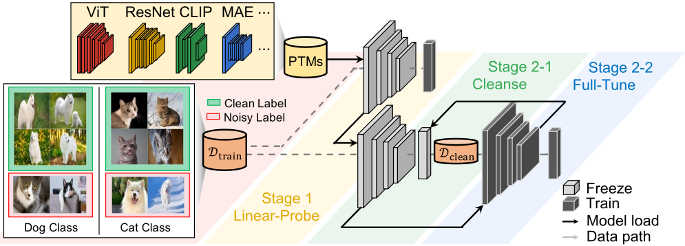
- The proposed method, fine-TUning pre-trained models for Robustness under Noisy labels (TURN), consists of two adaptation steps (as described in Figure 1): LP and then FFT. The LP step aims to adapt the model to the target task without compromising the integrity of the feature extractor, enabling the effective detection of noisy samples. The FFT step further enhances the feature extractor by updating entire trainable parameters, followed by dataset cleansing.
- Experimental results demonstrate the efficiency and robustness of the proposed method compared to existing LNL methods on various datasets, including synthetically noisylabeled datasets like CIFAR-100, as well as real-world datasets such as WebVision and Clothing1M.
2 Preliminary
Learningwith noisy labels. Let us denote the training dataset as Dtrain = ¶(xi↪ ¯ yi)♦Ni=1 , comprising N pairs of input images xi and their corresponding labels ¯ yi 2 ¶1↪ ▷ ▷ ▷ ↪C♦. In realworld scenarios, the given label ¯ yi can be corrupted due to various factors, such as human errors in crowd-sourced labeling systems. We use yi to denote the ground truth label for (xi↪ ¯ yi), which is not accessible during the training phase. It is widely acknowledged that models trained on noisy labeled datasets Dtrain using conventional classification loss functions, such as cross-entropy loss (LCE), often exhibit poor performance on test data. This limitation poses challenges when deploying such models in real-world scenarios. Therefore, training robust models capable of effectively handling noisy labeled datasets becomes essential.
1 A similar observation was noted in a previous study [Cheng et al., 2023], but their findings were only focused on a SimCLR model trained on the target dataset. However, we expand this to the models trained on different datasets (e.g., ImageNet) and various PTMs.
Pre-trained model and fine-tuning. In recent times, several PTMs have been proposed for image-related tasks, encompassing models trained using supervised learning (SL) [Dosovitskiy et al., 2021; Liu et al., 2021; Liu et al., 2022], selfsupervised learning (SSL) [He et al., 2022; Assran et al., 2022], and multimodal learning [Radford et al., 2021]. They have become accessible and demonstrated significant performance in classification tasks. To harness the power of the pre-trained feature extractor, two primary tuning methods are commonly employed: linear probing (LP) and full fine-tuning (FFT). We represent the classification model with a PTM as g(f(x; ✓); φ), where g(·; φ) denotes the linear classifier with its parameter φ, and the feature extractor f(·; ✓) has its parameter ✓. In LP, ✓ remains frozen and only φ is trained. In contrast, FFT involves tuning all trainable parameters, including both ✓ and φ. The advantages and disadvantages of LP and FFT are fundamentally distinct. LP has the strength of inexpensive computational cost thanks to the limited number of trainable parameters, but has rigid adaptability. On the other hand, FFT has strong adaptability, but requires a large amount of training resources.
3 Motivating Observation
In this section, our objective is to analyze the behavior of the feature extractor when tuned on severely or slightly noisy labels. We particularly focus on identifying the conditions that lead to improvements in the feature extractor. The key observations that form the basis of our investigation are summarized as follows.
(Obs 1) The presence of a high proportion of noisy labels can significantly distort the feature extractor when FFT is applied. (Obs 2) Conversely, when the noise ratio is not severe, FFT can effectively enhance the feature extractor, allowing it to construct class-wise clusters accurately.
Inspired by these observations, we propose a denoising algorithm for PTMs, which is elaborated in Section 4. In subsequent paragraphs, we provide detailed explanations for these two motivations. 2
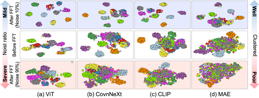
Experimental Setting. In our investigation, we performed experiments to evaluate the performance of several popular PTMs on a dataset with noisy labels. The considered PTMs include ViT-B/16 [Dosovitskiy et al., 2021], ConvNeXt-T [Liu et al., 2022], CLIP-ViT-B [Radford et al., 2021], and MAEViT-B [He et al., 2022]. To generate the noisy labeled dataset, we employ the symmetric label-flipping technique on the CIFAR-100 dataset. This technique randomly flips the labels of either 90% or 10% of the samples, resulting in different levels of label noise. We investigate the impact of noisy labels by visualizing the embedding of randomly sampled 10 classes from the test dataset using t-SNE [Van der Maaten and Hinton, 2008] plots. Each model is trained for 5 epochs following [Kumar et al., 2022].
(Obs 1) In the severe noise case, applying FFT results in distortion of the feature extractor. The distortion of the feature extractor occurs due to the incorrect supervision signals by the noisy labels. To gain a deeper understanding of this phenomenon, we employ t-SNE plots. In Figure 2, the middle row illustrates the initial feature extractor of each PTM, while the bottom row displays the features after applying FFT with 90% noisy labels. It can be seen that the features become mixed and less distinguishable. This effect is particularly evident when the initial clusters of the PTMs are already poorly defined, i.e., MAE. As a result, the application of FFT on a severely noisy dataset leads to a trained feature extractor that fails to adequately capture the intrinsic characteristics of the samples.
2 There was an observation of the impact of FFT and LP for PTMs [Kumar et al., 2022]. Its main focus is on scenarios where PTMs are fine-tuned on Dtrain ⇠ (X↪ Y) and tested on out-ofdistribution dataset, i.e., Dtest ⇠ (X 0 ↪ Y), where X 0 6= X . In contrast, we mainly focus on noisy label case, where the input images x in the training and testing datasets follow identical distribution while the labels in the training dataset is inaccurate.
(Obs 2) FFT improves the feature extractor when the target dataset has slight label noise. When dealing with minor label noise in the target dataset, applying FFT to the feature extractor yields improvements in constructing class-wise clusters effectively. The upper row of Figure 2 reveals that the models under examination exhibit a better construction of class-wise clusters compared to the middle row. This observation suggests that fine-tuning the feature extractor on a dataset with slight label noise can enhance its performance, enabling it to capture more meaningful features from each sample.
4 ProposedMethod: TURN
Based on the findings in Section 3, we can extract crucial strategies for the effective use of PTMs in noisy label datasets. First, if the training dataset is significantly contaminated with label noise (i.e., Obs 1), it is critical to avoid directly incorporating these noisy labels, as they can negatively impact the valuable feature extractor of PTMs. Hence, a buffer, such as LP, is needed to manage these highly noisy instances, as it allows the feature extractor to remain frozen. Second, when the training dataset exhibits relatively low label noise (i.e., Obs 2), FFT should be employed for task adaptation. This is due to the need for the feature extractor to be adjusted to the target dataset after FFT in the presence of minor noise. However, a key challenge remains: the lack of specific information on the noise label, including the intensity of the noise ratio. Therefore, the suggested approach to protect the feature extractor is a two-step procedure involving LP, followed by FFT. This section introduces our proposed two-step method, referred to as TURN (fine-TUning pre-trained models for Robustness under Noisy labels), aimed at addressing these challenges.
Algorithm 1 Pseudo code of TURN
Input: Dataset Dtrain = ¶(xi↪ ¯ yi)♦Ni=1 , Linear classifiers g(z; φ), Pre-trained feature extractor f(x; ✓), GMM threshold ⌧ , Linear probing epoch ELP, Full fine tuning epoch EFFT Output: Fine-tuned model g(f(·)) /* Step 1: Linear probing */ Extract feature zi = f(xi; ✓) for all samples (xi↪ ¯ yi) 2 Dtrain for e < ELP do Train the linear classifier g(zi; φ) under GCE Loss: LGCE(g(zi; φ)↪ ¯ yi) end /* Step 2: Select clean samples and FFT */ for e < EFFT do Extract per-sample loss for all samples in Dtrain Construct clean subset Dclean by using GMM with threshold ⌧ Train the model g(f(xj ; ✓); φ) under LCE(g(f(xj ; ✓)φ)↪ ¯ yj ) on Dclean = ¶(xj ↪ ¯ yj )♦
end
4.1 AlgorithmDescription
In this section, we provide a detailed explanation of the proposed algorithm. Briefly speaking, The algorithm consists of two main steps. In Step 1, the algorithm utilizes LP with an initialized fully connected layer, denoted as g(z; φ), where z represents the output of the frozen feature extractor f(x; ✓) for each input image x. Subsequently, in Step 2, the algorithm iteratively cleanses the training dataset and performs FFT on the entire model g(f(x; ✓); φ) using a subsampled dataset Dclean. The procedure of TURN is described in Algorithm 1.
Step 1: Linear probing. The first step of the algorithm serves two main objectives. Firstly, the objective is to obtain a classifier that can detect noisy labels, which is consistent with the approach taken by previous works that utilize a warm-up phase before detecting noisy labels [Li et al., 2020; Karim et al., 2022; Kim et al., 2021]. Second, during the training of the classifier for detecting noisy labels, it is crucial to ensure that the feature extractor is not distorted by noisy labels. To address this, we employ LP, which helps protect the feature extractor from being affected by severe label noise. As mentioned in Section 3, there is evidence that the feature extractor can be improved through FFT when applied to datasets with a small proportion of noisy labels. However, since the exact degree of label noise is unknown, we adopt a conservative approach by freezing the feature extractor until we have a classifier capable of detecting noisy labels.
Additionally, applying LP enhances efficiency, which is a key consideration derived from the inherent strengths of LP, as described in Section 2. Therefore, we employ the following implementation technique. Since the feature extractor remains frozen in this step, the extracted features of the input images remain unchanged. As a result, we pre-extract the features zi of input images xi as zi = f(xi; ✓) in advance, minimizing computational overhead during the subsequent steps.
Next, we update the parameters φ for ELP epochs by utilizing the Generalized Cross Entropy loss [Zhang and Sabuncu, 2018], denoted as LGCE = 1-g(zi;φ)q q , where q is a hyperparameter. GCE loss is used to mitigate the influence of noisy labels during linear classifier training. This step is crucial for effectively training the linear classifier, as it helps to clean the dataset in preparation for the subsequent steps.
Step 2: Cleansing and FFT In Step 2, the main objective is to improve the performance of the model by adapting it to the target dataset. As mentioned in Section 3, applying FFT to a dataset with a slight noise label enables the feature extractor to better adapt to the target dataset. Therefore, the remaining part of this step focuses on obtaining a sufficiently cleansed dataset. This stage is divided into two substeps: cleansing and FFT. In the cleansing phase, clean samples are selected from the given noisy dataset, while discarding the remaining samples. Following the cleansing phase, FFT is carried out on the selected clean subset, to improve the performance of the model on the target dataset. These two substeps are carried out for EFFT epochs iteratively. This is because a model that is trained better exhibits a greater ability to distinguish noisy labels.
Note that we can achieve efficiency by discarding the noisy labeled samples during the FFT procedure, leveraging the inherent strength of PTMs. As mentioned above, PTMs are highly capable of adapting to clean datasets using few-shot learning techniques. This allows the model to achieve successful performance even with a small portion of clean training samples. In the subsequent sections, we will provide a comprehensive description of each substep involved in the FFT process.
◦ Step 2-1: Selection of clean samples. To identify clean samples, we utilize a clustering algorithm based on the Gaussian Mixture Model (GMM), a commonly employed in previous research works [Li et al., 2020; Kim et al., 2021; Ahn and Yun, 2023]. This algorithm begins by calculating the loss for each sample, which is determined based on its noisy labels. This process allows us to distinguish between clean and noisy samples in the dataset.
After obtaining the per-sample loss, the next step involves fitting the GMM model using the calculated losses ¶`i♦Ni=1 . From this GMM model, we extract two Gaussian distributions for each class c, i.e., pcl and pch . Here, pcl represents the distribution with a lower mean value compared to pch . Utilizing these per-class distributions, we construct the clean dataset using the following procedure,
where Dc clean = ¶(xi↪ ¯ yi)♣pcl (`i) > ⌧ where ¯ yi = c♦. In this formulation, the threshold hyperparameter ⌧ is used, and the function U(D↪ n) denotes the uniform sampling function, which randomly selects n samples uniformly from the set D. It is worth noting that an equal number of samples is selected for each class from the set considered clean. This selection strategy is based on the principle emphasized in [Karim et al., 2022], which highlights the importance of maintaining a uniform distribution. Therefore, we set n = minc2¶1↪▷▷▷↪C♦ ♣Dc clean ♣↪ where ♣D♣ represents the cardinality of the set D.
◦ Step 2-2: FFT on the selected dataset Dclean. In Step 2-1, a clean subset is extracted from the noisy target dataset. This subset is obtained by reducing the proportion of noisy labels, thereby creating an environment conducive to performing FFT. With a reduced influence of noisy labels, the FFT process can be executed, allowing the model to adapt more effectively to the underlying clean samples present in the training dataset.
5 Experiments
In this section, we present empirical evaluations that showcase the superior performance of TURN. We begin by providing a detailed description of the LNL benchmarks and implementation in Section 5.1. Subsequently, in Section 5.2, we present the experimental results obtained from extensive evaluations. Further analyses to gain a deeper understanding of TURN are described in Appendix.
5.1 Experimental Setting
Datasets. We conduct an evaluation on the synthetically noised CIFAR-100 dataset, and real-world noisy labeled dataset, the Clothing 1M and WebVision datasets. For the CIFAR dataset, we introduce uniform random noise into a portion of the labels to simulate symmetric noise, asymmetric noise which flips the labels to specific classes [Liu et al., 2020]. To incorporate instance-dependent noise, we adopt the noise generation methodology described in [Cheng et al., 2021].
Architectures and baselines. In our evaluation, we consider several PTMs for each dataset, including ViT-B/16 [Dosovitskiy et al., 2021], ConvNeXt-T [Liu et al., 2022], MAE-ViTB [He et al., 2022], MSN-ViT-B [Assran et al., 2022], CLIPViT-B [Radford et al., 2021], and ResNet-50 [He et al., 2016]. In the case of CLIP model, we utilize the visual model. Among these architectures, we compare our proposed TURN with various previous methods, including Vanilla (trained on crossentropy loss), GCE [Zhang and Sabuncu, 2018], ELR [Liu et al., 2020], DivideMix [Li et al., 2020], and UNICON [Karim et al., 2022]. Additionally, we apply both FFT and LP to all algorithms for comparison. However, it is worth noting that DivideMix and UNICON require a significant number of feed-forwards for each sample, approximately 4 times and 8 times, respectively, with various data augmentation techniques. Due to the computational limitation, we utilize LP for both DivideMix and UNICON. For further details, please refer to Appendix B.
Implementation. To optimize the hyperparameters for each model, we utilize the Ray [Liaw et al., 2018] hyperparameter tuning tool. This allows us to identify the appropriate settings for parameters such as learning rate, weight decay, optimizer, and batch size. For each PTM, specific optimized hyperparameters and their search spaces are described in the Appendix A. Regarding the hyperparameter for TURN, namely GMM threshold, ⌧ = 0▷6, we adopt the value suggested in the DivideMix paper [Li et al., 2020], which initially introduced the GMM-based clean sample selection. For baselines, we run 5 epochs for FFT and 20 epochs for LP, while TURN is optimized 20 epochs of LP with 4 epochs for FFT in Step 2 to spend smaller computational cost compared to the baselines.
5.2 Classification Result
CIFAR datasets. For CIFAR-100 dataset, we include four noisy label cases {Symm 0▷6, Symm 0▷9, Asym 0▷4, Inst 0▷4}. The results shown in Table 2 demonstrate that TURN, when applied to various PTMs, consistently delivers high performance across different types and severities of noisy labels. Furthermore, the proposed method exhibits the superiority of the FFT and LP tuning mechanisms. Specifically, the ViT-B/16 model consistently outperforms others. As discussed in Section 3, in cases of severe label noise (i.e., Symm 90% noise), the LP-based approach generally yields more stable performance compared to FFT. Conversely, in cases of less severe label noise (e.g., Symm 60% noise), FFT tends to outperform LP. This tendency can be understood by Obs 1 that FFT under severe noise can distort the feature extraction. However, TURN approach consistently outperforms both cases. Therefore, it can be concluded that the sequential combination of LP followed by FFT is a valuable way for tuning PTMs on noisy datasets.
Real-world tasks. We evaluate the performance of TURN on larger datasets, namely Clothing1M and WebVision. The results in Table 3 consistently demonstrate that TURN improves performance on these datasets. This highlights the ability of TURN to handle noisy labels in real-world scenarios. However, some models, like MAE, MSN, and ResNet on Clothing1M, show a drop in performance due to the fine-grained nature compared to the training dataset (i.e., ImageNet). Nonetheless, our algorithm performs better by utilizing FFT in the second step.
5.3 Further Analysis
We deliver further analyses to answer the following keywords: (1) efficiency, (2) hyperparameter sensitivity (3) larger model case, and (4) ablation study. They are included in Appendix.
Larger model analysis. We also examine the performance of the proposed algorithm using larger models (ViT-L/16 and CLIP-ViT-L/14) on the CIFAR-100 dataset with 90% symmetric case. As shown in Table 4, the proposed algorithm consistently outperforms the other FFT and LP cases. Notably, when using larger models, the performance tends to improve compared to the results in Table 2. However, it is important to consider that larger models require more computation resources and time for tuning due to the increased number of model parameters.
Hyperparameter sensitivitiy. In the proposed method, we analyze three types of hyperparameters: (1) the number of epochs for LP denoted as ELP, (2) the number of epochs for FFT denoted as EFFT, and (3) the GMM threshold ⌧. Our experiments on CIFAR-100 with 90% symmetric noise reveal that increasing the number of epochs for LP improves performance until reaching 20 epochs, beyond which the gain becomes negligible. Similarly increasing the number of FFT epochs up to 5 provides similar performance due to the similar sample size per epoch. Moreover, increasing the GMM
| Tuning Type | CIFAR-100 | ||||||||
|---|---|---|---|---|---|---|---|---|---|
| Alg. | Symm. 0▷6 | Symm. 0▷9 | Asym. 0▷4 | Inst. 0▷4 | Symm. 0▷6 | Symm. 0▷9 | Asym. 0▷4 | Inst. 0▷4 | |
| ViT-B/16 | ConvNeXt-T | ||||||||
| CE | 88.45◦0.59 | 62.31◦1.51 | 61.25◦1.52 | 64.42◦0.14 | 79.12◦0.32 | 54.72◦1.01 | 68.31◦0.52 | 57.61◦0.40 | |
| FFT | GCE | 89.82◦1.32 | 46.51◦0.62 | 83.73◦0.31 | 1.31◦0.60 | 81.53◦0.52 | 62.31◦0.82 | 79.52◦0.73 | 1.17◦0.21 |
| ELR | 88.52◦0.18 | 63.52◦0.52 | 77.83◦0.52 | 83.34◦0.27 | 78.93◦0.68 | 51.52◦0.74 | 74.62◦0.42 | 67.14◦0.32 | |
| CE | 81.20◦0.49 | 64.17◦0.62 | 61.15◦1.24 | 61.62◦0.04 | 70.67◦0.69 | 53.14◦0.26 | 54.83◦0.14 | 62.15◦0.31 | |
| GCE | 83.19◦0.91 | 81.21◦0.15 | 76.32◦0.63 | 43.11◦0.20 | 73.76◦1.32 | 65.21◦0.83 | 70.26◦0.25 | 5.00◦0.05 | |
| LP | ELR | 81.23◦0.24 | 65.58◦0.62 | 64.37◦0.83 | 69.43◦0.00 | 70.95◦0.16 | 52.38◦0.83 | 57.15◦0.52 | 61.31◦0.21 |
| DMix | 84.31◦0.28 | 80.72◦0.52 | 82.62◦0.73 | 84.26◦0.32 | 74.92◦0.92 | 68.25◦1.14 | 72.41◦0.25 | 65.73◦0.52 | |
| UNC | 83.15◦0.46 | 80.23◦1.25 | 83.51◦1.18 | 84.32◦0.31 | 71.12◦0.71 | 60.35◦0.76 | 63.92◦0.29 | 69.25◦0.3 | |
| LP-FFT | Ours | 90.62◦0.42 | 84.35◦1.13 | 88.13◦1.00 | 87.57◦0.15 | 83.83◦0.52 | 70.01◦1.32 | 81.28◦1.12 | 73.40◦0.13 |
| MAE-ViT-B | MSN-ViT-B | ||||||||
| CE | 60.21◦0.52 | 7.58◦0.23 | 55.48◦0.52 | 50.70◦0.32 | 67.42◦0.28 | 5.52◦0.13 | 57.35◦0.74 | 62.24◦0.41 | |
| FFT | GCE | 58.47◦0.92 | 3.06◦0.41 | 60.54◦0.85 | 1.00◦0.00 | 65.51◦0.77 | 7.16◦0.32 | 61.58◦0.52 | 1.00◦0.00 |
| ELR | 63.24◦0.62 | 7.84◦0.13 | 61.47◦0.52 | 48.24◦0.52 | 67.19◦0.63 | 5.00◦0.24 | 70.58◦0.75 | 58.14◦0.42 | |
| CE | 48.31◦0.86 | 20.29◦0.15 | 38.98◦0.53 | 44.62◦0.75 | 60.01◦0.65 | 22.82◦0.62 | 47.72◦0.86 | 63.85◦0.53 | |
| GCE | 49.82◦0.73 | 14.13◦0.72 | 48.27◦0.65 | 1.79◦0.36 | 47.75◦0.86 | 14.15◦0.83 | 42.49◦0.82 | 1.45◦0.74 | |
| LP | ELR | 47.88◦0.72 | 17.26◦0.62 | 39.32◦0.83 | 46.52◦0.53 | 60.21◦0.46 | 20.72◦0.65 | 51.04◦0.25 | 61.13◦0.54 |
| DMix | 59.46◦0.93 | 24.89◦0.86 | 55.64◦0.72 | 51.28◦0.43 | 70.28◦0.52 | 42.58◦0.67 | 65.51◦0.85 | 61.45◦0.26 | |
| UNC | 37.13◦0.52 | 21.32◦0.57 | 34.21◦0.86 | 39.15◦1.24 | 67.15◦0.98 | 51.82◦0.96 | 61.02◦0.74 | 66.32◦1.23 | |
| LP-FFT | Ours | 64.33◦0.26 | 28.83◦0.75 | 65.97◦1.00 | 56.53◦1.32 | 79.52◦0.73 | 54.35◦0.64 | 75.33◦0.24 | 69.13◦1.42 |
| CLIP-ViT-B | ResNet-50 | ||||||||
| CE | 80.17◦0.50 | 26.84◦0.94 | 64.31◦0.85 | 72.66◦0.30 | 66.12◦1.32 | 0.75◦0.61 | 51.98◦1.07 | 56.12◦2.58 | |
| FFT | GCE | 81.56◦1.01 | 3.18◦0.68 | 78.35◦0.87 | 1.13◦0.12 | 55.78◦0.42 | 5.14◦1.52 | 57.04◦0.87 | 1.21◦0.25 |
| ELR | 76.24◦0.51 | 32.27◦1.18 | 75.38◦1.17 | 71.66◦0.56 | 65.38◦0.69 | 8.51◦1.59 | 61.21◦1.10 | 56.60◦1.55 | |
| CE | 74.24◦0.91 | 52.17◦1.18 | 53.99◦1.79 | 63.09◦1.33 | 67.19◦0.52 | 49.17◦1.70 | 53.52◦2.00 | 54.95◦2.22 | |
| GCE | 79.66◦1.13 | 65.49◦1.35 | 72.91◦0.36 | 19.87◦0.43 | 65.21◦1.52 | 49.32◦0.76 | 58.24◦2.19 | 57.58◦1.80 | |
| LP | ELR | 73.92◦1.21 | 51.94◦0.60 | 56.57◦2.67 | 65.11◦1.72 | 65.14◦0.93 | 49.53◦1.09 | 55.08◦1.49 | 54.51◦1.21 |
| DMix | 77.97◦0.99 | 69.55◦0.90 | 75.17◦1.70 | 71.12◦0.38 | 71.03◦0.92 | 56.54◦0.54 | 62.85◦1.45 | 60.40◦1.18 | |
| UNC | 73.54◦0.52 | 59.55◦1.07 | 67.37◦1.38 | 72.47◦2.68 | 70.03◦1.53 | 58.08◦0.92 | 66.41◦0.89 | 67.79◦0.61 | |
| LP-FFT | Ours | 84.12◦0.82 | 72.55◦1.45 | 78.41◦0.89 | 80.96◦1.97 | 73.32◦0.93 | 59.64◦0.60 | 69.38◦1.00 | 69.78◦0.76 |
threshold results in a correct subset of improved performance. Therefore, careful tuning of these hyperparameters can contribute to enhanced performance.
Component analysis. To evaluate the impact of each component of TURN, we conducted experiments on the CIFAR-100 dataset under 90% symmetric case. Specifically, we examined three components: (1) LP, (2) Cleansing, and (3) FFT. Regarding Cleansing, we explored different types: None (no cleansing), Once (cleansing once right before FFT), and Multiple (cleansing at the beginning of Step 2). The results, as shown in Table 5, indicate that the configuration involving all components achieves the best performance. Additionally, LP acts as a buffer to prevent the feature extractor from being distorted, as evidenced by the performance drop observed in the first row. When cleansing is omitted, a significant decrease in performance is also observed.
Training time. To assess the efficiency of the proposed algorithm, we examine the correlation between training time and test accuracy as depicted in Figure 3d. We run FFT on the CIFAR-100 benchmark under 90% noisy ratio. We run each algorithm for 5 epochs. As described in Figure 3d, TURN shows better performance (+2▷69% compared to UNICON) while spending the smallest training time (i.e., ⇥0▷12 compared to UNICON). This is because leveraging noisy labels by giving pseudo-labels for them, such as DivideMix and UNICON, requires a significant amount of time due to their computationally expensive nature. Furthermore, robust loss-based algorithms exhibit reduced computational costs compared to the pseudo-label based methods but they used entire training samples, while TURN utilize part of a clearer training dataset. This analysis emphasizes the efficiency of TURN.
6 RelatedWork
Learning with noisy labels. Noisy label problem has been explored extensively in recent researches [Li et al., 2020; Cheng et al., 2021; Kim et al., 2021; Xia et al., 2022; Karim et al., 2022; Cheng et al., 2023]. Existing methods mainly address this problem by (1) detecting corrupted instances and only using label information of clean examples [Li et al., 2020; Cheng et al., 2021; Kim et al., 2021; Xia et al., 2022] (2) designing loss functions [Zhang and Sabuncu, 2018; Wang et al., 2019; Zhou et al., 2021] or regularization terms [Liu et al., 2020; Ko et al., 2022; Cheng et al., 2023] with robust behaviors. Recently, the majority of the researches [Zheltonozhskii et al., 2022; Karim et al., 2022; Li et al., 2022; Tu et al., 2023; Huang et al., 2023] have focused on applying self-supervised approaches to construct robust feature extractors on label noise. The authors of [Zheltonozhskii et al., 2022; Ko et al., 2023] used pre-trained models to run semi-supervised approaches with the initial parameters from the SimCLR [Chen et al., 2020] and showed significant performances. However, these approaches may be over-complicated requiring hyperparameter tuning for different datasets, as well as significant computation resources.
| Clothing1M | |||||||||
|---|---|---|---|---|---|---|---|---|---|
| Architecture | CE | GCE | LP ELR | DivideMix | UNICON | CE | FFT GCE | ELR | LP+FFT Ours |
| ViT-B/16 | 67.83 / 67.54 | 67.46 / 67.46 | 66.91 / 66.91 | 68.13 / 68.13 | 68.42 / 68.42 | 68.98 / 68.98 | 69.74 / 69.74 | 68.73 / 68.73 | 70.28 / 70.28 |
| ConvNeXt-T | 64.82 / 64.81 | 64.59 / 64.59 | 64.17 / 64.17 | 66.12 / 65.42 | 67.33 / 66.92 | 68.80 / 68.80 | 68.92 / 68.92 | 69.19 / 68.52 | 69.63 / 69.63 |
| MAE-ViT-B | 5.06 / 5.06 | 5.92 / 5.92 | 8.28 / 8.28 | 8.04 / 8.04 | 8.52 / 8.52 | 61.31 / 61.31 | 60.80 / 60.80 | 61.51 / 61.51 | 61.96 / 61.96 |
| MSN-ViT-B | 6.77 / 6.77 | 6.20 / 6.20 | 7.64 / 7.64 | 6.42 / 6.42 | 6.31 / 6.31 | 66.88 / 63.38 | 67.06 / 65.41 | 66.32 / 66.32 | 69.13 / 69.13 |
| ResNet-50 | 7.08 / 7.08 | 7.18 / 7.18 | 6.68 / 6.68 | 8.13 / 8.13 | 8.24 / 8.24 | 66.10 / 66.02 | 66.19 / 66.19 | 66.19 / 66.19 | 66.31 / 66.31 |
| Architecture | CE | GCE | LP ELR | DivideMix | WebVision UNICON | CE | FFT GCE | ELR | LP+FFT Ours |
| ViT-B/16 | 84.62 / 84.48 | 84.32 / 84.24 | 84.48 / 84.32 | 84.72 / 84.72 | 85.68 / 85.68 | 84.20 / 83.04 | 83.40 / 83.40 | 84.92 / 83.72 | 85.96 / 85.92 |
| ConvNeXt-T | 85.24 / 85.24 | 85.12 / 85.04 | 86.28 / 86.28 | 86.40 / 86.40 | 86.24 / 86.24 | 84.00 / 82.68 | 85.40 / 84.92 | 84.52 / 83.44 | 87.16 / 86.44 |
| MAE-ViT-B | 48.00 / 48.00 | 47.32 / 47.28 | 49.76 / 49.76 | 59.40 / 58.44 | 56.96 / 53.80 | 67.48 / 65.64 | 63.16 / 62.84 | 67.80 / 67.80 | 69.45 / 68.45 |
| MSN-ViT-B | 77.40 / 77.40 | 74.40 / 74.40 | 74.00 / 74.00 | 76.56 / 76.40 | 77.72 / 77.34 | 77.04 / 77.80 | 72.28 / 72.28 | 74.88 / 72.28 | 78.36 / 75.40 |
| ResNet-50 | 84.88 / 84.72 | 81.68 / 81.68 | 84.96 / 84.96 | 85.16 / 85.16 | 85.04 / 85.04 | 78.00 / 76.44 | 77.04 / 70.92 | 80.44 / 77.44 | 85.36 / 85.36 |

| Method | CE | GCE | Linear Probing ELR | DMix | UNICON | CE | Full Fine-Tuning GCE | ELR | LP + FFT Ours |
|---|---|---|---|---|---|---|---|---|---|
| ViT-L/16 | 81.20 / 60.77 | 70.02 / 70.02 | 81.70 / 79.46 | 84.58 / 84.58 | 84.87 / 84.87 | 84.37 / 53.08 | 42.71 / 42.71 | 80.22 / 49.78 | 87.02 / 85.90 |
| CLIP-ViT-L/14 | 41.24 / 41.24 | 36.48 / 36.48 | 41.01 / 41.01 | 80.68 / 80.13 | 75.83 / 75.83 | 63.30 / 38.59 | 71.93 / 71.70 | 68.16 / 48.27 | 81.17 / 81.17 |
| LP | Cleansing | FFT | ViT-B/16 | CLIP-ViT-B |
|---|---|---|---|---|
| Multiple | 3 | 45.51 | 30.07 | |
| 3 | None | 3 | 45.90 | 47.47 |
| 3 | Once | 3 | 83.00 | 60.80 |
| 3 | Multiple | 3 | 83.33 | 72.17 |
Pre-trained visual models. Recently, several studies have demonstrated that PTMs, which are trained on the large image set (ImageNet), can learn universal visual representations that are useful for downstream computer vision tasks. This has eliminated the need to train a new model from scratch. With the advancement of computational power and development of deep models such as ViT[Dosovitskiy et al., 2021] and ConvNext [Liu et al., 2022], the capabilities of PTMs have greatly improved. Utilizing PTMs has been considered as an effective solution for multi-modal models such as CLIP [Radford et al., 2021] and Data2Vec [Baevski et al., 2022], which can effectively represent various types of domains. As researchers make pre-trained weights of PTMs available to the open-source community, there is growing interest in finding ways to effectively use these pre-trained weights.
7 Conclusion
This study introduces TURN, an algorithm designed to handle noisy labels using large pre-trained models. It focuses on robustly leveraging these models and minimizing noisy label effects. TURN uses linear probing and fine-tuning on a refined subset of the training dataset. Its enhanced performance is evident from experiments on CIFAR-100, Clothing 1M, and WebVision datasets, demonstrating both improved results and lower computational costs.
Acknowledgments
This work was supported by Institute of Information & communications Technology Planning & Evaluation (IITP) grant funded by the Korea government (MSIT) (No.2019-0-00075, Artificial Intelligence Graduate School Program (KAIST),
10%) and the Institute of Information & communications Technology Planning & Evaluation (IITP) grant funded by the Korea government (MSIT) (No. 2022-0-00871, Development of AI Autonomy and Knowledge Enhancement for AI Agent Collaboration, 90%)
@inproceedings{ijcai2024p403,
  title     = {Fine-tuning Pre-trained Models for Robustness under Noisy Labels},
  author    = {Ahn, Sumyeong and Kim, Sihyeon and Ko, Jongwoo and Yun, Se-Young},
  booktitle = {Proceedings of the Thirty-Third International Joint Conference on
               Artificial Intelligence, {IJCAI-24}},
  publisher = {International Joint Conferences on Artificial Intelligence Organization},
  editor    = {Kate Larson},
  pages     = {3643--3651},
  year      = {2024},
  month     = {8},
  note      = {Main Track},
  doi       = {10.24963/ijcai.2024/403},
  url       = {https://doi.org/10.24963/ijcai.2024/403},
}
TY - CPAPER TI - Fine-tuning Pre-trained Models for Robustness under Noisy Labels AU - Ahn, Sumyeong AU - Kim, Sihyeon AU - Ko, Jongwoo AU - Yun, Se-Young T2 - Proceedings of the Thirty-Third International Joint Conference on Artificial Intelligence, IJCAI-24 PB - International Joint Conferences on Artificial Intelligence Organization PY - 2024 SP - 3643 EP - 3651 DO - 10.24963/ijcai.2024/403 UR - https://doi.org/10.24963/ijcai.2024/403 ER -Copied
Machine-readable versions of this paper, for tools and AI agents:





