
Disentangling Domain and General Representations for Time Series Classification
Proceedings of the Thirty-Third International Joint Conference on Artificial Intelligence. Main Track. Pages 3834-3842.
https://doi.org/10.24963/ijcai.2024/424
Keywords
- Machine Learning: ML: Classification
- Machine Learning: ML: Deep learning architectures
- Machine Learning: ML: Time series and data streams
Abstract
Modeling time series data has become a very at tractive research topic due to its wide application, such as human activity recognition, financial forecasting and sensor-based automatic system monitoring. Recently deep learning models have shown great advances in modeling the time series data but they heavily depend on a large amount of labeled data. To avoid costly labeling, this paper explores domain adaptation from a labeled source domain to the unlabeled target domain on time series data. To achieve the goal, we propose a disentangled representation learning framework named CADT to disentangle the domain-invariant features from the domain-specific ones. Particularly, CADT is injected with a novel class-wise hypersphere loss to improve the generalization of the classifier from the source domain to the target domain. Intuitively, it restricts the source data of the same class within the same hypersphere and minimizes the radius of it, which in turn enlarges the margin between different classes and makes the decision boundary of both domains easier. We further devise several kinds of domain-preserving data augmentation methods to better capture the domain-specific patterns. Extensive experiments on two public datasets and two real-world applications demonstrate the effectiveness of the proposed model against several state-of-the-art baselines.
- [Arjovsky et al., 2017] Martín Arjovsky, Soumith Chintala, and Léon Bottou. Wasserstein generative adversarial net- works. In Proceedings of the 34th International Confer- ence on Machine Learning, ICML 2017, volume 70, pages 214-223, 2017.
- [Bai et al., 2018] Shaojie Bai, J. Zico Kolter, and Vladlen Koltun. An empirical evaluation of generic convolutional and recurrent networks for sequence modeling. CoRR, abs/1803.01271, 2018.
- [Bousmalis et al., 2017] Konstantinos Bousmalis, Nathan Silberman, David Dohan, Dumitru Erhan, and Dilip Kr- ishnan. Unsupervised pixel-level domain adaptation with generative adversarial networks. In 2017 IEEE Conference on Computer Vision and Pattern Recognition, CVPR 2017, pages 95-104, 2017.
- [Cai et al., 2021] Ruichu Cai, Jiawei Chen, Zijian Li, Wei Chen, Keli Zhang, Junjian Ye, Zhuozhang Li, Xiaoyan Yang, and Zhenjie Zhang. Time series domain adapta- tion via sparse associative structure alignment. In Pro- ceedings of the AAAI Conference on Artificial Intelligence, volume 35, pages 6859-6867, 2021.
- [Chen et al., 2016] Xi Chen, Yan Duan, Rein Houthooft, John Schulman, Ilya Sutskever, and Pieter Abbeel. In- fogan: Interpretable representation learning by informa- tion maximizing generative adversarial nets. In Advances in Neural Information Processing Systems 29, NIPS 2016, pages 2172-2180, 2016.
- [Fulcher and Jones, 2014] Ben D. Fulcher and Nick S. Jones. Highly comparative feature-based time-series classifica- tion. IEEE Transactions on Knowledge and Data Engi- neering, 26(12):3026-3037, 2014.
- [Ganin and Lempitsky, 2015] Yaroslav Ganin and Victor S. Lempitsky. Unsupervised domain adaptation by backprop- agation. In Proceedings of the 32nd International Confer- ence on Machine Learning, ICML 2015, volume 37, pages 1180-1189, 2015.
- [Glorot et al., 2011] Xavier Glorot, Antoine Bordes, and Yoshua Bengio. Domain adaptation for large-scale sen- timent classification: A deep learning approach. In Pro- ceedings of the 28th International Conference on Machine Learning, ICML 2011, pages 513-520, 2011.
- [Goodfellow et al., 2014] Ian J. Goodfellow, Jean Pouget- Abadie, Mehdi Mirza, Bing Xu, David Warde-Farley, Sherjil Ozair, Aaron C. Courville, and Yoshua Bengio. Generative adversarial networks. CoRR, abs/1406.2661, 2014.
- [He et al., 2016] Kaiming He, Xiangyu Zhang, Shaoqing Ren, and Jian Sun. Deep residual learning for image recog- nition. In Proceedings of the IEEE conference on computer vision and pattern recognition, pages 770-778, 2016.
- [Hochreiter and Schmidhuber, 1997] Sepp Hochreiter and Jürgen Schmidhuber. Long short-term memory. Neural computation, 9(8):1735-1780, 1997.
- [Jin et al., 2022] Xiaoyong Jin, Youngsuk Park, Danielle Maddix, Hao Wang, and Yuyang Wang. Domain adap- tation for time series forecasting via attention sharing. In International Conference on Machine Learning, pages 10280-10297. PMLR, 2022.
- [Kim and Jeong, 2021] Mooseop Kim and Chi Yoon Jeong. Label-preserving data augmentation for mobile sensor data. Multidimensional Systems and Signal Processing, 32(1):115-129, 2021.
- [Koltchinskii and Panchenko, 2002] Vladimir Koltchinskii and Dmitry Panchenko. Empirical margin distributions and bounding the generalization error of combined classifiers. The Annals of Statistics, 30(1):1-50, 2002.
- [Kwapisz et al., 2011] Jennifer R Kwapisz, Gary M Weiss, and Samuel A Moore. Activity recognition using cell phone accelerometers. ACM SigKDD Explorations Newsletter, 12(2):74-82, 2011.
- [Lee et al., 2019] Chen-Yu Lee, Tanmay Batra, Moham- mad Haris Baig, and Daniel Ulbricht. Sliced wasserstein discrepancy for unsupervised domain adaptation. In IEEE Conference on Computer Vision and Pattern Recognition, CVPR 2019, pages 10285-10295, 2019.
- [Li et al., 2021] Jingjing Li, Mengmeng Jing, Hongzu Su, Ke Lu, Lei Zhu, and Heng Tao Shen. Faster domain adap- tation networks. IEEE Transactions on Knowledge and Data Engineering, pages 1-1, 2021.
- [Li et al., 2022] Keqiuyin Li, Jie Lu, Hua Zuo, and Guangquan Zhang. Dynamic classifier alignment for un- supervised multi-source domain adaptation. IEEE Trans- actions on Knowledge and Data Engineering, pages 1-1, 2022.
- [Lin and Jung, 2017] Yuan-Pin Lin and Tzyy-Ping Jung. Im- proving eeg-based emotion classification using condi- tional transfer learning. Frontiers in human neuroscience, 11:334, 2017.
- [Liu et al., 2019] Hongfu Liu, Ming Shao, Zhengming Ding, and Yun Fu. Structure-preserved unsupervised domain adaptation. IEEE Transactions on Knowledge and Data Engineering, 31(4):799-812, 2019.
- [Liu et al., 2022] Shenghua Liu, Bin Zhou, Quan Ding, Bryan Hooi, Zheng bo Zhang, Huawei Shen, and Xueqi Cheng. Time series anomaly detection with adversarial re- construction networks. IEEE Transactions on Knowledge and Data Engineering, pages 1-1, 2022.
- [Long et al., 2015] Mingsheng Long, Jianmin Wang, Ji- aguang Sun, and Philip S. Yu. Domain invariant trans- fer kernel learning. IEEE Transactions on Knowledge and Data Engineering, 27(6):1519-1532, 2015.
- [Long et al., 2016] Mingsheng Long, Jianmin Wang, Yue Cao, Jiaguang Sun, and Philip S. Yu. Deep learning of transferable representation for scalable domain adaptation. IEEE Transactions on Knowledge and Data Engineering, 28(8):2027-2040, 2016.
- [Mathieu et al., 2016] Michaël Mathieu, Junbo Jake Zhao, Pablo Sprechmann, Aditya Ramesh, and Yann LeCun. Disentangling factors of variation in deep representation using adversarial training. In Advances in Neural Informa- tion Processing Systems 29, NIPS 2016, pages 5041-5049, 2016.
- [Ozyurt et al., 2023] Yilmazcan Ozyurt, Stefan Feuerriegel, and Ce Zhang. Contrastive learning for unsupervised do- main adaptation of time series. ICLR, 2023.
- [Pan and Yang, 2010] Sinno Jialin Pan and Qiang Yang. A survey on transfer learning. IEEE Transactions on Knowl- edge and Data Engineering, 22(10):1345-1359, 2010.
- [Patel et al., 2015] Vishal M. Patel, Raghuraman Gopalan, Ruonan Li, and Rama Chellappa. Visual domain adapta- tion: A survey of recent advances. IEEE Signal Processing Magazine, 32(3):53-69, 2015.
- [Purushotham et al., 2017] Sanjay Purushotham, Wilka Car- valho, Tanachat Nilanon, and Yan Liu. Variational re- current adversarial deep domain adaptation. In 5th Inter- national Conference on Learning Representations, ICLR 2017, 2017.
- [Qian et al., 2019] Hangwei Qian, Sinno Jialin Pan, Bing- shui Da, and Chunyan Miao. A novel distribution- embedded neural network for sensor-based activity recog- nition. In Proceedings of the Twenty-Eighth International Joint Conference on Artificial Intelligence, IJCAI 2019, pages 5614-5620, 2019.
- [Qiang et al., 2021] Wenwen Qiang, Jiangmeng Li, Chang- wen Zheng, Bing Su, and Hui Xiong. Robust local pre- serving and global aligning network for adversarial do- main adaptation. IEEE Transactions on Knowledge and Data Engineering, pages 1-1, 2021.
- [Ragab and Eldele, 2022] Mohamed Ragab and Emadeldeen Eldele. Subject-wise Sleep Stage Data, 2022.
- [Reyes-Ortiz et al., 2016] Jorge-L Reyes-Ortiz, Luca Oneto, Albert Samà, Xavier Parra, and Davide Anguita. Transition-aware human activity recognition using smart- phones. Neurocomputing, 171:754-767, 2016.
- [Sun and Saenko, 2016] Baochen Sun and Kate Saenko. Deep coral: Correlation alignment for deep domain adap- tation. In Gang Hua and Hervé Jégou, editors, Computer Vision -ECCV 2016 Workshops, pages 443-450, Cham, 2016. Springer International Publishing.
- [Sun et al., 2015] Shiliang Sun, Honglei Shi, and Yuanbin Wu. A survey of multi-source domain adaptation. Infor- mation Fusion, 24:84-92, 2015.
- [Tan et al., 2022] Chang Wei Tan, Angus Dempster, Christoph Bergmeir, and Geoffrey I Webb. Multirocket: multiple pooling operators and transformations for fast and effective time series classification. Data Mining and Knowledge Discovery, 36(5):1623-1646, 2022.
- [Tonutti et al., 2019] Michele Tonutti, Emanuele Ruffaldi, Alessandro Cattaneo, and Carlo Alberto Avizzano. Ro- bust and subject-independent driving manoeuvre antici- pation through domain-adversarial recurrent neural net- works. Robotics Auton. Syst., 115:162-173, 2019.
- [Tran et al., 2017] Luan Tran, Xi Yin, and Xiaoming Liu. Disentangled representation learning GAN for pose- invariant face recognition. In 2017 IEEE Conference on Computer Vision and Pattern Recognition, CVPR 2017, pages 1283-1292, 2017.
- [Tzeng et al., 2017] Eric Tzeng, Judy Hoffman, Kate Saenko, and Trevor Darrell. Adversarial discriminative domain adaptation. In 2017 IEEE Conference on Com- puter Vision and Pattern Recognition, pages 2962-2971, 2017.
- [Wang et al., 2018] Fang Wang, Sheng-hua Zhong, Jianfeng Peng, Jianmin Jiang, and Yan Liu. Data augmentation for eeg-based emotion recognition with deep convolu- tional neural networks. In MultiMedia Modeling: 24th In- ternational Conference, MMM 2018, Bangkok, Thailand, February 5-7, 2018, Proceedings, Part II 24, pages 82-93. Springer, 2018.
- [Wilson et al., 2020] Garrett Wilson, Janardhan Rao Doppa, and Diane J. Cook. Multi-source deep domain adaptation with weak supervision for time-series sensor data. In The 26th ACM SIGKDD Conference on Knowledge Discovery and Data Mining, KDD '2020, pages 1768-1778, 2020.
- [Yan et al., 2021] Yuguang Yan, Hanrui Wu, Yuzhong Ye, Chaoyang Bi, Min Lu, Dapeng Liu, Qingyao Wu, and Michael Kwok-Po Ng. Transferable feature selection for unsupervised domain adaptation. IEEE Transactions on Knowledge and Data Engineering, pages 1-1, 2021.
- [Yang et al., 2021] Shuai Yang, Kui Yu, Fuyuan Cao, Lin Liu, Hao Wang, and Jiuyong Li. Learning causal represen- tations for robust domain adaptation. IEEE Transactions on Knowledge and Data Engineering, pages 1-1, 2021.
- [Zellinger et al., 2017] Werner Zellinger, Thomas Grub- inger, Edwin Lughofer, Thomas Natschläger, and Susanne Saminger-Platz. Central moment discrepancy (CMD) for domain-invariant representation learning. In 5th Inter- national Conference on Learning Representations, ICLR 2017, 2017.
- [Zhang et al., 2021] Qian Zhang, Wenhui Liao, Guangquan Zhang, Bo Yuan, and Jie Lu. A deep dual adversarial network for cross-domain recommendation. IEEE Trans- actions on Knowledge and Data Engineering, pages 1-1, 2021.
- [Zhuang et al., 2019] Fuzhen Zhuang, Zhiyuan Qi, Keyu Duan, Dongbo Xi, Yongchun Zhu, Hengshu Zhu, Hui Xiong, and Qing He. A comprehensive survey on trans- fer learning. CoRR, abs/1911.02685, 2019.
References were extracted automatically from the PDF and may contain errors.
Full text extracted automatically from the PDF; figures, tables and equations may differ. The PDF is the version of record.
1 Introduction
Time series data is prevalent in real-world applications like human activity recognition, financial prediction, and manufacturing sensor monitoring. Recently, deep learning models such as long short-term memory networks (LSTM) [Hochreiter and Schmidhuber, 1997] and 1-dimensional convolution networks (Conv1D) [Bai et al., 2018] have shown promising advances in time series classification and forecasting.
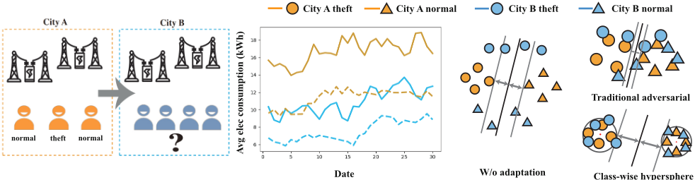
Using the mentioned deep learning models effectively typically requires a large amount of labeled data. Labeling time series data demands more manual effort from experts due to the consecutive property of time series data [Lin and Jung, 2017; Wang et al., 2018; Kim and Jeong, 2021]. Fig. 1(a) demonstrates the challenge of identifying electricity theft, highlighting the extensive effort required for labeling. Detecting such behavior often demands prolonged on-site investigations by domain experts. Applying models trained on labeled data from one city to others is complex due to variations in electricity consumption patterns influenced by economic status, weather conditions, and electricity prices, leading to potential misclassification or failure to detect electricity thieves.
∗Corresponding author.
In view of the great labeling cost and the significant domain gap of time series data, we propose to study unsupervised domain adaptation (UDA) for time series data. UDA aims to perform the task on the unlabeled target domain by leveraging the labeled data of a source domain. Compared to existing pretraining methods, UDA does not require labeled target domain datasets for fine-tuning. Additionally, compared to zero-shot pretraining, UDA can better leverage the correlation between the source and target domains, thereby achieving improved performance. Back to our example, if the model can mitigate the distribution divergence between the source domain and target domain. Intuitively, electricity thieves share some common characteristics no matter in which city they live. For example, their overall electric power consumption is higher than that of normal residents which can be treated as domain-invariant patterns across domains. However, thieves of different areas have their specific electricity consumption patterns and theft modes which are domain-specific patterns. Thus, how to capture the domaininvariant patterns across the source and the target domain with remarkable domain-specific patterns is crucial.
To achieve the goal, we disentangle the representation learning of the domain-invariant and the domain-specific patterns. The motivation is depicted through the electricity theft example in Fig. 1(b), showcasing the variations in average daily electricity consumption over a month for regular users and electricity thieves in two distinct Chinese cities. City A, with an adequate label set, serves as the source domain, while city B represents the target domain devoid of any labels. No matter what users we consider, we can see that city A consumes much more electrical power than city B. If the difference between such domain-specific patterns is ignored, we might derive the wrong domain-invariant pattern that users who consume electricity of more than 13 Kilowatt a) Detecting electricity theft by UDA
- Electricity consumption in a month c) Learning domain-invariant representations
Figure 1: Illustration of domain adaptation and its challenges by taking electricity theft detection task as the example.
hours (kWh) are thieves. As a result, the electricity thieves of city B will be easily misclassified as normal users. To unfold the correct domain-invariant pattern such as the higher power consumption of the thieves compared with the normal users, we need to disentangle the domain-specific patterns from the domain-invariant ones, i.e., to perform UDA by disentangled representation learning, which is inspired by the similar studies in the image data [Chen et al., 2016; Tran et al., 2017] and the textural data [Mathieu et al., 2016]. To the best of our knowledge, we are the first to explore disentangled representation learning for time series domain adaptation. Despite the success of such studies on other types of data, disentangling the domain-specific representations from the general (domain-invariant) representations by the widely-adopted adversarial learning [Tzeng et al., 2017; Ganin and Lempitsky, 2015] without considering the classes of data instances, may cause the domain-invariant representations cannot be discriminated between different classes of the prediction task. Efforts to minimize domain differences can hinder the classifier's ability to distinguish between different classes due to the adversarial loss. Then, the source classifier's capacity to generalize knowledge to the target classifier diminishes. [Koltchinskii and Panchenko, 2002].
To address the above challenge, we propose to inject the class-wise hypersphere loss into the traditional adversarial learning, expecting to learn an easier decision boundary in the source domain as well as the target domain illustrated in the right bottom of Fig. 1(c). To be specific, in the source domain, we restrict the data instances of the same class in the same hypersphere and minimize the radius of it to compact the instances of the same class instead of all the instances regardless of their classes. By doing this, the margin between different classes could be relatively enlarged.
Formally, we propose a Class-wise Adversarial learning framework for Domain adaptation in Time-series data (CADT), to learn the domain-invariant representations by the supervision of the class labels. CADT is equipped with coupled interactive networks to enable the disentangled representation learning, which extracts the domain-specific features and the domain-invariant features by different networks respectively. An additional class-wise hypersphere loss is injected into the traditional adversarial learning loss to enhance the discrimination ability of the task classifier. To capture various domain-specific time series patterns, we devise several kinds of domain-preserving data augmentation methods. Overall, our main contributions are summarized as follows:
- To the best of our knowledge, we are the first to explore the disentangled domain-invariant and domain-specific representation learning for UDA in time series data.
- We propose an adversarial learning framework, CADT, equipped with coupled interactive networks for disentangled learning. It includes the class-wise hypersphere loss to improve model generalization and is enhanced by data augmentation to capture domain-specific patterns.
- We conduct extensive experiments on two public datasets and two real-world application datasets (electricity theft detection and electric vehicle accident prediction). The results show that CADT consistently outperforms several state-of-the-art baseline methods.
2 RelatedWorks
Unsupervised domain adaptation is a specific instance of transfer learning [Zhuang et al., 2019; Long et al., 2015] with labeled source domain data and unlabeled target domain data, where the mapping representation spaces are shared but their marginal distributions remain different due to the dataset shift [Yang et al., 2021; Yan et al., 2021; Liu et al., 2019]. Abundant previous works survey on this topic in computer vision (CV) [Patel et al., 2015; Sun et al., 2015] and natural language processing (NLP) applications [Glorot et al., 2011; Pan and Yang, 2010]. Typically, the mapping representation involves minimizing the measure of discrepancy between source features and target features [Zellinger et al., 2017; Lee et al., 2019; Li et al., 2022]. With the remarkable success in deep learning, many studies utilize the deep neural networks as a feature extractor to learn representative domain-invariant representations [Sun and Saenko, 2016; Li et al., 2021; Long et al., 2016]. Inspired by the generative adversarial networks (GANs) [Goodfellow et al., 2014;
Source domain
Target domain
Figure 2: The overall architecture of CADT. It contains three components: interactive networks to learn domain-invariant and domain-specific features for source and target data simultaneously, domain discriminator with class-wise hyperspheres to adversarially guide the model to learn domain-invariant features, and domain classifier with data augmentations to help the model learn plentiful domain-specific features.
Arjovsky et al., 2017], many UDA approaches [Tzeng et al., 2017; Ganin and Lempitsky, 2015; Bousmalis et al., 2017; Zhang et al., 2021; Qiang et al., 2021] are proposed to learn domain-invariant representation based on adversarial learning. Specifically, these approaches consist of a feature extractor, a domain discriminator, and a label predictor. The feature extractor acts as the generator in GAN, whose goal is to produce domain-invariant representation in the mapping space to fool the domain discriminator. The domain discriminator is trained to detect if the extracted feature is from the source or the target domain. The domain adaptation and deep feature learning are within one training process. Furthermore, the label predictor predicts the label of training source samples based on features that are both invariant to domains and discriminative. Although time series data is abundant in real-world applications [Liu et al., 2022; Fulcher and Jones, 2014], few works focused on UDA for temporal data. Specifically, considering the sequential structure of temporal data, previous works [Purushotham et al., 2017; Tonutti et al., 2019] leveraged recurrent neural network as the feature extractor. CoDATS [Wilson et al., 2020] leverage 1dimensional convolutional neural networks as the feature extractor. CoDATS achieves competitive performances on several human activity recognition tasks. However, these methods have vulnerable domain-invariant representations due to shared feature extractor and adversarial architecture. Additionally, a particular design for time series data is also essential due to its consecutive property.
3 Our Approach
In this section, we propose a novel CADT to fulfill domain adaptation for time series data.
Problem definition. In domain adaptation setting, there are two different data distributions: P from the source domain and Q from the target domain. We are given by ns labeled samples ˆ P = {(xsi , ys i )}ns i=1 drawn from the source distribution where ys i ∈ {1, · · · , k} is the label of k-class classification, and nt unlabeled samples ˆQ = {xti }nt i=1 drawn from the target distribution. Our goal is to predict the label ˆ yt of each sample xt ∈ ˆQ.
3.1 Model Overview
We illustrate the architecture of our method CADT in Fig. 2. The cornerstone of CADT is the coupled interactive networks that aims to learn the domain-invariant representations and the domain-specific representations respectively for instances from two domains. The two networks, therefore, interact with each other to exchange their information. Each of the two interactive networks will output two representations hs and ht, corresponding to the instances from the source domain and the target domain respectively. To achieve the goal of disentangling the domain-invariant representations from domain-specific ones, we design a domain discriminator D and a domain classifier C to guide the interactive networks. The domain discriminator ensures that the target domaininvariant representations cannot be distinguished from the source domain-invariant representations. In contrast, the domain classifier aims to preserve the characteristics of each domain within their respective domain-specific representations. We enhance the discrimination ability by using a task classifier T to leverage label information from the source domain and equipping the domain discriminator with a set of class-wise hyperspheres to of the task classifier. To better capture the plentiful domain-specific patterns, we design several domain-preserving data augmentations.
3.2 Coupled Interactive Networks
Most existing time-series domain adaptation models adopt a deep neural network as the single extractor to directly capture domain-invariant features [Wilson et al., 2020; Purushotham et al., 2017; Tonutti et al., 2019]. These methods neglect domain-specific information, which is also very important for domain adaptation as illustrated in Fig. 1(b). In order to extract both the domain-invariant and domain-specific features, we propose a couple of interactive networks.
Generally, domain-invariant and domain-specific features shall reflect different characteristics of the given time series data. In particular, domain-invariant features tend to describe the "high-level" patterns, which underlie the superficial data and are difficult to be discovered intuitively. These features need to capture the abstract, underlying patterns that are shared between different domains which can be complex and not easily understood intuitively (e.g., the essential characteristics of electricity stealing). Domain-specific features, such as the scale and amplitude of electricity usage data, typically represent more concrete and identifiable information compared to domain-invariant features. These features can be specific to a particular domain and may not be applicable to other domains. Deep neural network may overfit on irrelevant domain-specific noises while learning these "low-level" features. Inspired by this, we propose to use a shallow neural network to capture the "low-level" domain-specific representations and use a deep neural network to capture the "highlevel" domain-invariant representations respectively.
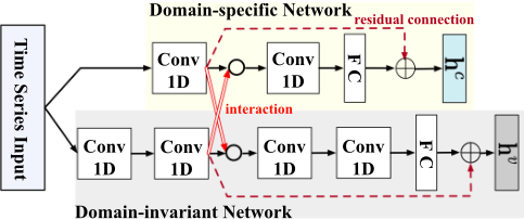
Intuitively, the network that is responsible for extracting domain-invariant features requires domain-specific information to understand which characteristics are truly common, and vice versa. We therefore make the two networks communicate with each other to share their information by adding interactions among their different layers. Fig. 3 shows the architecture of the interactive networks. We use hck to denote the output of the k-th layer of the domain-specific network and use hvj to indicate the output of the j-th layer of the domain-invariant network. The operation of interaction between two networks can be expressed as
where Finter(hck , hvj ) corresponds to passing the information of hck to hvj , Fk,j is the transform function which can be implemented by a sub-network or other forms, and ◦ is defined as concatenation.
Note that this interaction results in a blend of domaininvariant and domain-specific representations due to the gradient flow between the two networks during backpropagation in model learning. We add a residual connection [He et al., 2016] between the interactive layer and the output layer, allowing the network's loss to directly influence the interactive layer and lower layers, thus preserving the characteristics of features before interaction.
3.3 Domain-invariant Representations Learning
Adversarial Learning. Idea of adversarial learning is used in prior UDA methods [Wilson et al., 2020; Purushotham et al., 2017]. We use Hv (x) to denote the domain-invariant feature output by the network from the current time point. Then the output of the domain discriminator is D(Hv (x)). To distinguish the source data from the target data, we should minimize the following objective in discriminator:
On the contrary, the interactive networks are trying to make the domain-invariant features indistinguishable. It has the opposite objective from the discriminator, i.e.,
Besides, for a source data instance xs , its domain-invariant feature Hv (xs ) is also put into the task classifier to predict the task label T (Hv (xs )). Given the ground truth label ys , we optimize the classifier by:
where ℓ is the loss function which is usually instantiated as the cross-entropy loss.
By iteratively optimizing the domain discriminator and the interactive networks, we can obtain inseparable domaininvariant representations. However, the classification margin of the task classifier may be decreased by the discriminator. The task classifier forces the data instances with different classes in the source domain to be separated from each other, expecting to make the correct decision boundary. On the contrary, the discriminator favors tightening the distances between all the instances regardless of their classes so that their domains cannot be distinguished. Extremely, when all the instances are collapsed to the same embedding, the discriminator thoroughly loses its discrimination ability. [Koltchinskii and Panchenko, 2002].
Class-wise Hyperspheres. To address the above issue of the existing adversarial learning, we propose to inject a class-wise hyperspheres constraint into the adversarial learning. The general idea is to restrict source instances of the same class being projected into the same hyphersphere in the domain-invariant feature space, so that the adversarial learning cannot narrow the gaps between different classes. The class-wise hyperspheres constraint is applied to the labeled source data. As for the target data, once the source data are restricted in several hyperspheres (Fig. 2(b)), each target data will be placed into one of the hyperspheres in order to confuse the discriminator (Fig. 2(c)). Eventually, all the source data and target data are projected into the hyperspheres with a large margin (Fig. 2(d)). This approach helps to reduce the distribution discrepancy between the source and target domains in the domain-invariant representation space, thereby improving the model's generalization ability. Moreover, by increasing the distances among hyperspheres representing different categories, we can enlarge the margin of classification boundaries among different categories of data. This allows the model to make more precise distinctions on the target data, rather than ambiguous classifications, leading to improved classification performance.
| S | T | CNN | RNN | DDNN | MultiRocket | RDANN | VRADA | SASA | CoDATS | DAF | CLUDA | CADT |
|---|---|---|---|---|---|---|---|---|---|---|---|---|
| CHARGE | ||||||||||||
| 1 | 2 | 44.46±4.7 | 47.40±4.0 | 33.19±2.7 | 36.57±1.6 | 34.39±4.9 | 51.10±6.4 | 21.10±6.9 | 50.24±0.7 | 24.45±0.1 | 39.04±3.1 | 52.29±1.3 |
| 1 | 3 | 42.43±3.9 | 38.67±4.2 | 26.03±2.1 | 26.66±2.0 | 23.93±3.4 | 57.48±3.6 | 17.86±2.9 | 43.98±1.8 | 20.32±0.1 | 31.48±3.2 | 49.72±2.9 |
| 2 | 3 | 52.27±3.5 | 55.19±1.9 | 30.32±1.6 | 44.52±1.0 | 26.17±4.5 | 50.23±1.8 | 17.16±0.9 | 47.57±6.6 | 20.30±0.1 | 57.79±8.2 | 60.86±6.7 |
| 2 | 1 | 65.56±13 | 72.93±3.6 | 38.56±2.9 | 53.54±4.5 | 33.11±8.9 | 70.53±10 | 16.60±5.2 | 68.43±4.1 | 28.06±0.1 | 40.04±1.2 | 73.36±1.3 |
| 3 | 2 | 54.70±3.9 | 54.60±4.7 | 36.48±1.8 | 39.81±1.5 | 52.47±5.0 | 51.62±11 | 25.64±0.4 | 52.60±3.3 | 24.44±0.1 | 45.92±8.0 | 54.77±2.1 |
| 3 | 1 | 34.84±21 | 54.79±11 | 34.19±4.4 | 49.71±7.5 | 38.21±7.0 | 77.65±8.7 | 25.79±4.2 | 54.65±3.8 | 28.46±1.2 | 44.19±1.3 | 58.49±2.3 |
| ELEC | ||||||||||||
| D | C | 62.24±0.7 | 63.33±0.3 | 63.06±0.4 | 62.90±0.3 | 62.66±0.1 | 59.19±4.7 | 69.39±3.1 | 72.79±2.5 | 82.67±16 | 66.54±0.4 | 93.81±1.2 |
| C | D | 54.60±1.7 | 53.49±0.3 | 53.45±0.2 | 54.24±0.8 | 52.88±0.2 | 79.02±13 | 63.16±1.2 | 62.86±4.6 | 75.39±20 | 60.36±1.0 | 90.08±1.3 |
| D | B | 53.17±5.0 | 47.23±0.2 | 48.43±0.8 | 48.23±0.7 | 46.93±0.1 | 56.84±3.5 | 44.04±2.7 | 63.38±3.8 | 90.71±14 | 57.36±2.2 | 85.79±3.7 |
| B | D | 55.77±1.0 | 53.98±0.3 | 55.24±1.2 | 54.91±0.4 | 53.46±0.2 | 71.86±17 | 59.43±4.2 | 65.23±3.9 | 69.81±22 | 67.232±2.5 | 80.20±3.0 |
| A | E | 57.58±0.6 | 57.21±0.1 | 58.79±0.5 | 56.73±0.2 | 56.95±0.2 | 51.85±2.1 | 60.04±1.6 | 61.15±1.2 | 83.44±11 | 65.06±1.5 | 75.83±2.5 |
| E | A | 56.16±1.1 | 53.81±0.4 | 56.40±1.3 | 53.60±0.8 | 53.56±0.7 | 50.20±4.6 | 55.60±2.3 | 61.57±3.0 | 89.26±12 | 66.97±0.8 | 81.61±2.8 |
| UCIHAR | ||||||||||||
| 2 | 4 | 53.08±5.0 | 48.08±1.8 | 56.17±5.8 | 80.43±2.3 | 39.25±3.1 | 46.25±5.6 | 51.78±2.3 | 77.65±2.7 | 30.15±7.8 | 63.19±2.2 | 88.67±1.1 |
| 26 | 3 | 45.65±7.6 | 45.03±4.3 | 61.78±4.8 | 13.06±3.5 | 37.53±5.4 | 53.56±6.2 | 46.93±1.6 | 74.62±2.5 | 27.50±9.0 | 76.16±1.8 | 84.31±1.1 |
| 7 | 25 | 37.73±6.4 | 34.29±3.1 | 63.82±6.6 | 37.58±5.5 | 28.28±1.0 | 40.70±6.6 | 54.72±2.9 | 57.60±6.1 | 29.08±7.2 | 61.29±3.5 | 82.23±2.0 |
| 16 | 9 | 49.21±7.0 | 56.91±3.7 | 54.25±8.6 | 70.03±2.0 | 37.96±6.4 | 41.09±5.3 | 50.65±1.2 | 78.12±2.4 | 28.86±7.4 | 63.75±1.9 | 82.65±3.5 |
| 6 | 23 | 51.0±5.5 | 46.25±7.0 | 74.53±4.4 | 73.04±0.5 | 37.62±3.1 | 50.00±3.5 | 59.38±2.7 | 70.49±5.5 | 32.99±5.4 | 70.54±1.9 | 90.93±2.8 |
| 7 | 8 | 53.86±7.0 | 58.32±4.3 | 76.99±4.4 | 10.76±1.8 | 46.79±6.0 | 47.22±6.6 | 65.42±3.9 | 79.37±3.3 | 39.14±6.0 | 74.53±1.6 | 85.39±3.4 |
| 13 | 7 | 66.56±7.4 | 69.29±2.7 | 78.51±7.3 | 21.17±4.4 | 68.47±5.5 | 49.37±6.2 | 71.59±2.8 | 88.12±1.3 | 43.82±13 | 74.99±3.5 | 91.40±2.4 |
| 13 | 29 | 51.34±7.2 | 56.43±4.7 | 71.87±5.8 | 44.95±7.6 | 46.90±3.9 | 49.81±11 | 62.73±5.6 | 81.87±1.3 | 37.68±9.5 | 77.42±1.6 | 88.62±5.1 |
| WISDM | ||||||||||||
| 9 | 18 | 61.99±3.4 | 65.97±2.0 | 56.75±12 | 75.94±2.9 | 55.50±7.4 | 40.42±7.3 | 41.70±2.9 | 75.31±2.8 | 33.75±3.3 | 50.07±4.1 | 72.65±2.2 |
| 31 | 11 | 45.82±11 | 41.67±4.0 | 59.60±13 | 57.85±3.0 | 40.23±1.6 | 42.73±6.9 | 38.09±2.5 | 60.70±6.5 | 38.16±0.6 | 57.42±2.1 | 73.28±0.3 |
| 2 | 6 | 66.53±1.1 | 50.12±4.7 | 69.40±2.9 | 69.03±3.3 | 50.43±4.2 | 65.15±7.1 | 60.32±1.1 | 82.12±2.0 | 48.65±7.0 | 71.32±1.4 | 81.81±5.1 |
| 7 | 25 | 49.72±12 | 59.49±7.1 | 64.60±1.9 | 39.73±5.3 | 47.46±7.0 | 48.04±7.3 | 34.41±0.9 | 71.56±4.6 | 39.84±5.6 | 47.97±2.0 | 89.53±1.2 |
| 3 | 27 | 55.68±12 | 63.28±3.1 | 46.15±4.5 | 53.97±8.2 | 56.06±7.4 | 48.12±8.6 | 38.10±4.5 | 76.87±1.2 | 40.43±0.7 | 64.84±3.5 | 70.87±7.7 |
| 22 | 8 | 75.57±5.5 | 46.56±3.2 | 64.53±9.2 | 14.81±1.0 | 43.48±2.9 | 49.11±10 | 38.64±3.7 | 59.63±2.3 | 46.30±6.1 | 61.87±2.0 | 87.29±1.3 |
| 6 | 23 | 61.05±3.8 | 46.40±5.5 | 70.19±4.2 | 72.23±0.4 | 51.09±5.7 | 67.14±3.8 | 57.98±3.9 | 73.24±2.5 | 49.45±12 | 69.06±0.7 | 78.90±7.3 |
| 27 | 20 | 62.23±7.9 | 63.33±4.6 | 71.66±5.3 | 72.50±0.7 | 54.89±2.6 | 56.92±12 | 53.65±4.1 | 91.92±0.7 | 51.30±17 | 62.03±3.1 | 95.72±1.4 |
| Sleep-EDF | ||||||||||||
| 0 | 17 | 64.28±0.2 | 62.54±0.7 | 61.98±0.5 | 61.92±0.1 | 62.47±0.4 | 41.45±9.5 | 48.04±1.5 | 63.43±0.2 | 36.65±0.3 | 54.34±0.3 | 64.47±0.3 |
| 16 | 15 | 75.22±0.1 | 74.09±0.6 | 74.01±0.1 | 71.32±0.1 | 71.18±0.6 | 35.49±2.0 | 38.69±1.5 | 73.56±1.6 | 29.88±2.0 | 59.83±0.9 | 73.49±1.1 |
| 1 | 6 | 53.85±0.5 | 59.45±1.4 | 57.26±0.5 | 56.09±0.4 | 54.19±1.5 | 48.62±1.3 | 45.88±0.2 | 52.37±1.1 | 42.81±8.5 | 49.10±0.8 | 61.19±0.5 |
| 6 | 8 | 61.45±0.3 | 61.26±0.4 | 60.32±0.3 | 58.69±0.2 | 58.85±1.1 | 45.18±3.8 | 43.99±0.6 | 60.43±0.3 | 30.18±7.6 | 47.12±0.6 | 62.55±0.7 |
| 18 | 1 | 60.66±0.3 | 61.41±0.8 | 58.24±0.7 | 56.15±0.1 | 58.81±0.3 | 50.89±1.1 | 50.37±0.8 | 61.84±0.6 | 45.46±15 | 50.43±0.6 | 62.58±0.5 |
| 12 | 14 | 49.99±1.4 | 52.42±0.8 | 49.87±0.8 | 40.47±0.4 | 40.02±2.1 | 34.3±8.2 | 41.66±1.3 | 49.71±2.9 | 39.77±7.6 | 42.83±0.6 | 61.07±0.7 |
| 15 | 19 | 69.38±0.1 | 67.53±0.2 | 67.12±0.1 | 66.69±0.1 | 66.3±0.3 | 61.48±0.9 | 43.0±0.7 | 69.21±0.1 | 25.09±10 | 57.19±0.1 | 68.32±0.2 |
| 18 | 14 | 54.84±0.5 | 53.59±0.7 | 53.65±0.8 | 49.71±0.6 | 54.79±1.8 | 39.93±3.9 | 41.0±2.8 | 54.49±0.5 | 36.09±8.6 | 46.32±0.7 | 58.75±0.3 |
Formally, given a source dataset ˆ P with k classes of labeled data, our goal is to minimize the radius of the hypersphere for each class in domain-invariant feature space. The hyperspheres center of j-th class is cj and the corresponding radius is Rj. For simplicity, we use ˆ P j to denote the source instances whose label y is j. Then the objective of class-wise hypersphere with penalty is as follows:
The first term Rj minimizes the radius directly, while the second term is a soft penalty to restrict source data inside the sphere. Specifically, we calculate the distance of each source domain-invariant feature Hv (xs ) to its class center cys, then penalize features with distance larger than Rj by measuring max{0, ∥Hv (xs ) - cys ∥2 - R2 j }, and σ is a hyper-parameter controlling the trade-off between the penalty term and radius.
3.4 Domain-specific Representations Learning
In our framework, the domain-specific features are learned through the objective of predicting the data from either the source or the target. For simplicity, we use Hc (x) to denote the domain-specific feature output by the network. The output of the domain classifier is C(Hc (x)). Then the objective of the domain classifier is to minimize:
Optimizing this objective alone cannot ensure that the model captures the domain-specific features fully, since there are usually several domain characteristics, not just one. But once the model learns a particular characteristic that is totally different between source and target, the model stops learning other domain knowledge because it has already made a distinction between the two domains.
Intuitively, this issue can be solved by encouraging the model to learn features from different observation data each time. To be specific, we design the following domainpreserving data augmentation methods on domain classifier:
- Time-series window cropping: We randomly crop several slices from the original temporal data and paste them all as a new instance. This method tend to capture local domain characteristics existing in some segments like oscillation.
- Shuffling: We split time series data into some segments and then perform re-ordering to generate a synthetic time series. This method tends to capture local domain knowledge.
- Adding noise: We add noises like Gaussian noise and white noise to avoid our network capturing local noise as the domain-specific pattern considering that time series data is long-lasting and may contain noisy patterns like impulses.
- Segment reversing: We randomly perform reversing on some segments along the time-axis of data. This method aims to eliminate the temporal information and preserve the frequency information which is invariant to reversing, such as amplification and phase spectrum.
Overall Objective. We review all parts of our model and give an overall learning objective. Our model is optimized by adversarial learning. In the first stage, we optimize the model components except for the domain discriminator, the objective is to minimize:
In the second stage, we optimize the discriminator and fix other components, the objective is to minimize Ldis. The two stages are optimized iteratively. The whole learning algorithm of CADT is presented in the appendix.
4 Experiments
In this section, we conduct sufficient experiments to validate the effectiveness of the proposed model.
4.1 Experimental Setup
Datasets In our experiments, we utilize five datasets: CHARGE and ELEC from industrial practice, and UCIHAR [Reyes-Ortiz et al., 2016], WISDM [Kwapisz et al., 2011], SleepEDF [Ragab and Eldele, 2022] from publicly available datasets. Details of datasets will be provided in the supplementary materials 1 .
1 The code and supplementary materials are available at https: //github.com/IJCAI-CADT/cadt
| Dataset | CNN | w/o CH | w/o CIN | CADT |
|---|---|---|---|---|
| CHARGE | 49.04 | 49.61 | 56.99 | 56.50 |
| UCIHAR | 48.83 | 76.81 | 85.04 | 85.17 |
| WISDM | 71.10 | 77.00 | 76.99 | 78.59 |
Baselines We compare our proposed method with five types of baselines. The first category comprises deep learning networks with no adaptation, including CNN, RNN, DDNN [Qian et al., 2019], and MultiRocket [Tan et al., 2022]. MultiRocket is a fast time series classification (TSC) algorithm known for achieving state-of-the-art accuracy. We design these baselines to serve as a lower bound, revealing the gap of data distribution between source domain and target domain. The second type is RNN-based domain adaptation methods including R-DANN [Tonutti et al., 2019], VRADA [Purushotham et al., 2017] SASA [Cai et al., 2021]. Other types are CNN-based (CoDATS [Wilson et al., 2020]), attention-based (DAF [Jin et al., 2022]) domain adaptation methods and TCN-based (CLUDA [Ozyurt et al., 2023]). The implementation detailed will be presented in the supplementary materials.
4.2 Performance Comparison
We compare the performance of CADT with other baselines on public and industrial datasets. Tab. 1 shows that on the CHARGE dataset, our method achieves the best accuracy. especially in challenging scenarios.
The ELEC dataset includes 5 cities with varying economic conditions and regulatory intensities related to electricity theft. Our model outperforms all baseline methods, achieving the highest acc score . This demonstrates its adaptability to domains with different economic situations and geographical locations.
We use two common human activity recognition. From Tab. 1 , we find that CoDATS outperforms RNN-based methods, and our CADT outperforms all other baselines, showcasing the superiority of our disentangled CADT model. Additionally, we observe that CNN-based networks without adaptation can sometimes perform well, especially when participants have very similar health conditions.
The Sleep-EDF dataset is particularly unique; we observed that it is highly susceptible to negative transfer, resulting in suboptimal performance for transfer models other than CADT and CoDATS. However, overall, our model still achieves optimal performance.
4.3 Ablation Study
In this section, we validate the effectiveness of our method by demonstrating the performance influence of several components contributing to our method. Additionally, we provide an intuitive understanding of our learned hidden representations by projecting them into two-dimensional embeddings.
Effectiveness of coupled interactive networks. We investigate the effectiveness of our coupled interactive networks a) Domain-invariant w/o CH
b) Domain-invariant with CH
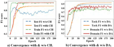
Figure 6: Convergence analysis for training and testing.
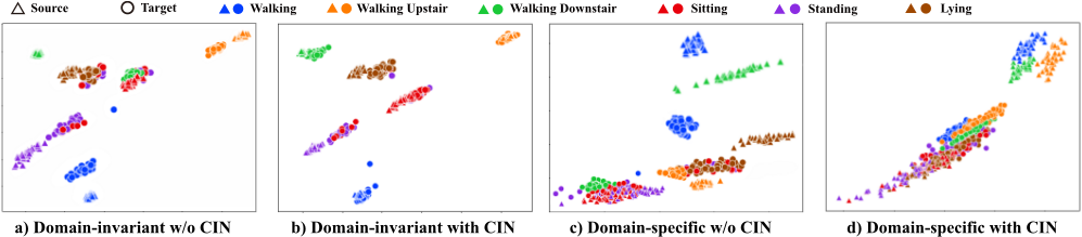
(CIN) for learning domain-specific and domain-invariant features. Initially, we compare the performance by removing the domain-specific component ("w/o CIN"). Results in Tab. 2 show reduced precisions in both datasets. We further give an intuition in Fig. 4 by projecting learned features linearly into a 2-dimensional space. By comparing Fig. 4(a) and Fig. 4(b), we find that CIN reduces the domain-invariant gap between the source and target domain. However, leveraging CIN helps to pull in the distance between them. We also drop the domain-invariant component of our model and compare the learned domain-specific features in Fig. 4(c) and Fig. 4(d). Additionally, the learned domain-specific features contain less class information in Fig. 4(d) since the distance among different categories is closer.
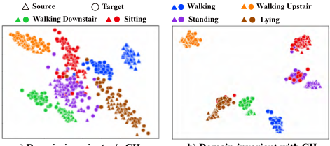
Effectiveness of class-wise hypersphere. We explore the effectiveness of class-wise hyperspheres (CH). "w/o CH" refers to without the class-wise hyperspheres constraint (CH). Results in Tab. 2 show that CH significantly improves our ability to predict target labels. In Fig. 5(a), without CH, domain-invariant features are dense and hard to distinguish.
Fig. 5(b) shows that features of each class are restricted into a very compact cluster and features from different classes are far away in the latent space. Furthermore, we also display the process of convergence with and without CH. Fig. 6(a) shows that leveraging class-wise hyperspheres makes the curve more stable and achieves a better performance. In contrast, the performances without hyperspheres are very unstable, because the classification margin is small and the classifier learned in the source data is easy to make wrong predictions on the target data.
Effectiveness of temporal data augmentation. Temporal data augmentation methods are designed for better learning of domain information. We hope that the augmented data can help the model learn plentiful domain-specific features. We compare the performance and convergence of using data augmentation or not. Fig. 6(b) displays that temporal data augmentation helps the model learn better domain-specific features for domain classification,
5 Conclusion
In this paper, we propose CADT, a time-series domain adaptation framework that disentangles domain-invariant representations from domain-specific ones using coupled interactive networks. We employ adversarial learning with a novel class-wise hypersphere constraint to learn domain-invariant representations, and introduce domain-preserving data augmentation methods. Our extensive experiments on two public datasets and three real-world applications demonstrate the effectiveness of CADT compared to several state-of-the-art baselines.
Acknowledgements
This work is supported by National Natural Science Foundation of China (No. 62176233, No. 62441605).
Contribution Statement
Youmin Chen and Xinyu Yan contributed equally to this work.
@inproceedings{ijcai2024p424,
  title     = {Disentangling Domain and General Representations for Time Series Classification},
  author    = {Chen, Youmin and Yan, Xinyu and Yang, Yang and Zhang, Jianfeng and Zhang, Jing and Pan, Lujia and Li, Juren},
  booktitle = {Proceedings of the Thirty-Third International Joint Conference on
               Artificial Intelligence, {IJCAI-24}},
  publisher = {International Joint Conferences on Artificial Intelligence Organization},
  editor    = {Kate Larson},
  pages     = {3834--3842},
  year      = {2024},
  month     = {8},
  note      = {Main Track},
  doi       = {10.24963/ijcai.2024/424},
  url       = {https://doi.org/10.24963/ijcai.2024/424},
}
TY - CPAPER TI - Disentangling Domain and General Representations for Time Series Classification AU - Chen, Youmin AU - Yan, Xinyu AU - Yang, Yang AU - Zhang, Jianfeng AU - Zhang, Jing AU - Pan, Lujia AU - Li, Juren T2 - Proceedings of the Thirty-Third International Joint Conference on Artificial Intelligence, IJCAI-24 PB - International Joint Conferences on Artificial Intelligence Organization PY - 2024 SP - 3834 EP - 3842 DO - 10.24963/ijcai.2024/424 UR - https://doi.org/10.24963/ijcai.2024/424 ER -Copied
Machine-readable versions of this paper, for tools and AI agents:





