
SpecAR-Net: Spectrogram Analysis and Representation Network for Time Series
Proceedings of the Thirty-Third International Joint Conference on Artificial Intelligence. Main Track. Pages 3917-3925.
https://doi.org/10.24963/ijcai.2024/433
Keywords
- Machine Learning: ML: Representation learning
- Machine Learning: ML: Convolutional networks
Abstract
Representing temporal-structured samples is essential for effective time series analysis tasks. So far, recurrent networks, convolution networks and transformer-style models have been successively applied in temporal data representation, yielding notable results. However, most existing methods primarily focus on modeling and representing the variation patterns within time series in the time domain. As a highly abstracted information entity, 1D time series couples various patterns such as trends, seasonality, and dramatic changes (instantaneous high dynamic), it is difficult to exploit these highly coupled properties merely by analysis tools on purely time domain. To this end, we present Spectrogram Analysis and Representation Network (SpecAR-Net). SpecAR-Net aims at learning more comprehensive representations by modeling raw time series in both time and frequency domain, where an efficient joint extraction of time-frequency features is achieved through a group of learnable 2D multi-scale parallel complex convolution blocks. Experimental results show that the SpecAR-Net achieves excellent performance on 5 major downstream tasks i.e., classification, anomaly detection, imputation, long- and short-term forecasting. Code and appendix are available at https://github.com/Dongyi2go/SpecAR_Net.
- [Abdulaal et al., 2021] Ahmed Abdulaal, Zhuanghua Liu, and Tomer Lancewicki. Practical approach to asyn- chronous multivariate time series anomaly detection and localization. Proceedings of the 27th ACM SIGKDD Con- ference on Knowledge Discovery & Data Mining, 2021.
- [Aksan and Hilliges, 2019] Emre Aksan and Otmar Hilliges. Stcn:stochastic temporal convolutional networks. In Inter- national Conference on Learning Representations (ICLR), 2019.
- [Albert Gu and Re., 2022] Karan Goel Albert Gu and Christopher Re. Efficiently modeling long sequences with structured state spaces. In International Conference on Learning Representations, 2022.
- [Bagnall et al., 2018] Anthony Bagnall, Anh Dau, Jason Lines, Michael Flynn, James Large, Aaron Bostrom, Paul Southam, and Eamonn Keogh. The uea multivariate time series classification archive, 2018, 10 2018.
- [Bai et al., 2018] Shaojie Bai, J. Kolter, and Vladlen Koltun. An empirical evaluation of generic convolutional and re- current networks for sequence modeling. 03 2018.
- [Cai et al., 2020] Ling Cai, Krzysztof Janowicz, Gengchen Mai, Bo Yan, and Rui Zhu. Traffic transformer: Captur- ing the continuity and periodicity of time series for traffic forecasting. Transactions in GIS, 24, 06 2020.
- [Challu et al., 2023] Cristian Challu, Kin G. Olivares, Boris Oreshkin, Federico Ramirez, Max Canseco, and Artur Dubrawski. Nhits: Neural hierarchical interpolation for time series forecasting. Proceedings of the AAAI Confer- ence on Artificial Intelligence, 37:6989-6997, 06 2023.
- [Chen and Shi, 2021] Wei Chen and Ke Shi. Multi-scale at- tention convolutional neural network for time series clas- sification. Neural Networks, 136:126-140, 2021.
- [Cook et al., 2020] Andrew A. Cook, Göksel Mısırlı, and Zhong Fan. Anomaly detection for iot time-series data: A survey. IEEE Internet of Things Journal, 7(7):6481-6494, 2020.
- [Dempster et al., 2020] Angus Dempster, Franc ¸ois Petitjean, and Geoffrey Webb. Rocket: exceptionally fast and accu- rate time series classification using random convolutional kernels. Data Mining and Knowledge Discovery, 34, 09 2020.
- [Franceschi et al., 2019] Jean-Yves Franceschi, Aymeric Dieuleveut, and Martin Jaggi. Unsupervised scalable representation learning for multivariate time series. In H. Wallach, H. Larochelle, A. Beygelzimer, F. d'Alché- Buc, E. Fox, and R. Garnett, editors, Advances in Neural Information Processing Systems, volume 32.
- Curran Associates, Inc., 2019.
- [Gasparin et al., 2021] Alberto Gasparin, Slobodan Lukovic, and Cesare Alippi. Deep learning for time series forecast- ing: The electric load case. CAAI Transactions on Intelli- gence Technology, 7, 09 2021.
- [Hochreiter and Schmidhuber, 1997] Sepp Hochreiter and Jürgen Schmidhuber. Long short-term memory. Neural Computation, 9(8):1735-1780, 1997.
- [Hochreiter, 1998] S. Hochreiter. The vanishing gradient problem during learning recurrent neural nets and problem solutions. International Journal of Uncertainty, Fuzziness and Knowledge-Based Systems, 06(2):-, 1998.
- [Hundman et al., 2018] Kyle Hundman, Valentino Con- stantinou, Christopher Laporte, Ian Colwell, and Tom Soderstrom. Detecting spacecraft anomalies using lstms and nonparametric dynamic thresholding. pages 387-395, 07 2018.
- [Lai et al., 2018a] Guokun Lai, Wei-Cheng Chang, Yiming Yang, and Hanxiao Liu. Modeling long-and short-term temporal patterns with deep neural networks. pages 95- 104, 06 2018.
- [Lai et al., 2018b] Guokun Lai, Wei-Cheng Chang, Yiming Yang, and Hanxiao Liu. Modeling long-and short-term temporal patterns with deep neural networks. In The 41st international ACM SIGIR conference on research & devel- opment in information retrieval, pages 95-104, 2018.
- [Liu et al., 2022a] Shizhan Liu, Hang Yu, Cong Liao, Jian- guo Li, Weiyao Lin, Alex X Liu, and Schahram Dust- dar. Pyraformer: Low-complexity pyramidal attention for long-range time series modeling and forecasting. In Inter- national Conference on Learning Representations, 2022.
- [Liu et al., 2022b] Yong Liu, Haixu Wu, Jianmin Wang, and Mingsheng Long. Non-stationary transformers: Rethink- ing the stationarity in time series forecasting. ArXiv, abs/2205.14415, 2022.
- [Livieris et al., 2020] Ioannis E. Livieris, Emmanuel G. Pin- telas, and Panagiotis P. Pintelas. A cnn-lstm model for gold price time-series forecasting. Neural Computing and Applications, 32:17351 -17360, 2020.
- [Makridakis et al., 2018] Spyros Makridakis, Evangelos Spiliotis, and Vassilios Assimakopoulos. The m4 com- petition: Results, findings, conclusion and way forward. International Journal of Forecasting, 34(4):802-808, 2018.
- [Mallet and others, 1999] Stephane Mallet et al. A wavelet tour of signal processing. Wavelet Analysis & Its Applica- tions), New York: Academic,, 1999.
- [Mathur and Tippenhauer, 2016] Aditya P. Mathur and Nils Ole Tippenhauer. Swat: a water treatment testbed for research and training on ics security. In 2016 International Workshop on Cyber-physical Systems for Smart Water Networks (CySWater), pages 31-36, 2016.
- [Maté and Jimeńez, 2021] Carlos Maté and Lucía Jimeńez. Forecasting exchange rates with the imlp: New empiri- cal insight on one multi-layer perceptron for interval time series (its). Engineering Applications of Artificial Intelli- gence, 104:104358, 2021.
- [Nikita Kitaev and Levskaya, 2020] Lukasz Kaiser Nikita Kitaev and Anselm Levskaya. Reformer: The efficient transformer. In International Conference on Learning Representations, 2020.
- [Oreshkin et al., 2019] Boris Oreshkin, Dmitri Carpo, Nico- las Chapados, and Yoshua Bengio. N-beats: Neural basis expansion analysis for interpretable time series forecast- ing. 05 2019.
- [Stoean et al., 2020] Ruxandra Stoean, Catalin Stoean, Miguel Atencia, Roberto Rodríguez-Labrada, and Gon- zalo Joya. Ranking information extracted from uncertainty quantification of the prediction of a deep learning model on medical time series data. Mathematics, 8(7), 2020.
- [Su et al., 2019] Ya Su, Youjian Zhao, Chenhao Niu, Rong Liu, Wei Sun, and Dan Pei. Robust anomaly detection for multivariate time series through stochastic recurrent neu- ral network. Proceedings of the 25th ACM SIGKDD In- ternational Conference on Knowledge Discovery & Data Mining, 2019.
- [Thill et al., 2021] Markus Thill, Wolfgang Konen, Hao Wang, and Thomas Bäck. Temporal convolutional autoen- coder for unsupervised anomaly detection in time series. Applied Soft Computing, 112:107751, 2021.
- [Wang et al., 2022] Jingyang Wang, Xiaolei Li, Jiazheng Li, Qiuhong Sun, and Haiyao Wang. Ngcu: A new rnn model for time-series data prediction. Big Data Research, 27:100296, 2022.
- [Woo et al., 2022] Gerald Woo, Chenghao Liu, Doyen Sa- hoo, Akshat Kumar, and Steven C. H. Hoi. Etsformer: Exponential smoothing transformers for time-series fore- casting. 2022.
- [Wu et al., 2021] Haixu Wu, Jiehui Xu, Jianmin Wang, and Mingsheng Long. Autoformer: Decomposition transform- ers with Auto-Correlation for long-term series forecasting. In Advances in Neural Information Processing Systems, 2021.
- [Wu et al., 2022] Haixu Wu, Jialong Wu, Jiehui Xu, Jianmin Wang, and Mingsheng Long. Flowformer: Linearizing transformers with conservation flows, 02 2022.
- [Wu et al., 2023] Haixu Wu, Tengge Hu, Yong Liu, Hang Zhou, Jianmin Wang, and Mingsheng Long. Timesnet: Temporal 2d-variation modeling for general time series analysis. In The Eleventh International Conference on Learning Representations, ICLR 2023, Kigali, Rwanda, May 1-5, 2023. OpenReview.net, 2023.
- [Xu et al., 2022] Jiehui Xu, Haixu Wu, Jianmin Wang, and Mingsheng Long. Anomaly transformer: Time series anomaly detection with association discrepancy. In Inter- national Conference on Learning Representations, 2022.
- [Yu et al., 2021] Wennian Yu, Il Yong Kim, and Chris Mechefske. Analysis of different rnn autoencoder vari- ants for time series classification and machine prognostics. Mechanical Systems and Signal Processing, 149:107322, 2021.
- [Zeng, 2023] Chen M. Zhang L. Xu Q. Zeng, A. Are trans- formers effective for time series forecasting? Proceed- ings of the AAAI Conference on Artificial Intelligence, 37:11121-11128, 06 2023.
- [Zhang et al., 2022] T. Zhang, Yizhuo Zhang, Wei Cao, J. Bian, Xiaohan Yi, Shun Zheng, and Jian Li. Less is more: Fast multivariate time series forecasting with light sampling-oriented mlp structures. ArXiv, abs/2207.01186, 2022.
- [Zhou et al., 2021a] Haoyi Zhou, Shanghang Zhang, Jieqi Peng, Shuai Zhang, Jianxin Li, Hui Xiong, and Wan- cai Zhang. Informer: Beyond efficient transformer for long sequence time-series forecasting. In Proceedings of the AAAI conference on artificial intelligence, volume 35, pages 11106-11115, 2021.
- [Zhou et al., 2021b] Haoyi Zhou, Shanghang Zhang, Jieqi Peng, Shuai Zhang, Jianxin Li, Hui Xiong, and Wancai Zhang. Informer: Beyond efficient transformer for long sequence time-series forecasting. In The Thirty-Fifth AAAI Conference on Artificial Intelligence, AAAI 2021, Virtual Conference, volume 35, pages 11106-11115. AAAI Press, 2021.
- [Zhou et al., 2022] Tian Zhou, Ziqing Ma, Qingsong Wen, Xue Wang, Liang Sun, and Rong Jin. FEDformer: Fre- quency enhanced decomposed transformer for long-term series forecasting. In Proc. 39th International Conference on Machine Learning (ICML 2022), 2022.
References were extracted automatically from the PDF and may contain errors.
Full text extracted automatically from the PDF; figures, tables and equations may differ. The PDF is the version of record.
1 Introduction
With the advent of the era of "Internet of Things" and "Comprehensive Perception", various sensors have been extensively deployed and utilized, leading to an explosive growth in the scale of time series [Cook et al., 2020]. Extracting valuable information from massive time series has become increasingly crucial. As a result, the time series analysis has attracted a growing number of researchers. Currently, time series analysis has been widely applied in numerous fields, e.g., finance [Livieris et al., 2020], electricity [Cai et al., 2020], transportation [Gasparin et al., 2021], and the healthcare sector [Stoean et al., 2020], etc.
Recently, deep learning is playing a crucial role in time series analysis. With the powerful feature representation capability, many deep time series learning methods have been proposed and achieved great success in classification, anomaly detection, short/long-term forecasting, etc. One typical category of these methods is based on recurrent neural networks (RNNs) [Wang et al., 2022; Yu et al., 2021], where the sequence modeling is completed by recursively encoding the first-order dependency between the preceding and subsequent elements. However, when modeling long-term sequences, it is easy to encounter gradient vanishing and explosion problems, and it is also difficult to enjoy the advantages of parallel processing [Hochreiter, 1998]. Another typical category is the convolution-based methods [Aksan and Hilliges, 2019; Thill et al., 2021], which can easily process sequential data in parallel. However, limited by the computation mechanism of shared convolutions in the local receptive fields, convolution models are often insufficient to characterize the longterm relationships. To overcome those shortcomings of recurrent and convolutional networks, the Self-Attention (SA) based Transformer [Liu et al., 2022a; Liu et al., 2022b] has been proposed. Transformer balances the long-term dependency encoding capability and the benefits of parallel computing, resulting in widely used backbone in various sequence modeling tasks. However, time series is coupled with multiple patterns, and the temporal dependencies captured by point-by-point representation and aggregation are often submerged [Wu et al., 2021].
As a highly abstract information body, time series couple multiple components such as trend (overall envelope), periodicity (multiple frequency components), mutagenicity (high frequency components), etc. Considering such highlycoupled property, it is almost impossible for pure-timedomain learning models to achieve complete semantic representation from time series. To overcome such limitation, introducing frequency domain analysis into modern deep backbones is proven to be an effective technical approach, and has become a current research trend. There are two notable works among these efforts, FEDformer [Zhou et al., 2022] and TimesNet [Wu et al., 2023]. Motivated by the fact that time series tend to have sparsity in frequency domain, FEDformer uses a small mount of randomly selected frequency components to reduce the complexity of time-domain SA from O(N 2 ) to O(N), resulting in a more agile model than Informer (O(log(N)N)). In the meanwhile, FEDformer keeps both low and high frequency components. By exploiting the posterior of Fourier transform, TimesNet constructs a 2D period-time space by folding the time series according to the dominant periods and conducts multi-scale 2D convolution to capture the intra-period- and inter-period-dependency.
In summary, both methods are eventually trying to achieve better sequence representation by using a selected frequency components, whether in a prior way [Zhou et al., 2022] or a posterior (data-driven) way [Wu et al., 2023]. And from the experimental results, the data-driven selection mechanism can achieve better results. While none of these approaches discuss whether the patterns of chosen frequency components over time, i.e., the joint characteristics of timefrequency domain, are helpful to the downstream tasks. In particular, TimesNet solely use the frequencies with high response values via Fourier transform to select dominant periodic components from time series. The subsequent modeling process is still carried out in the time domain, utilizing the data repeatedly guided by significant periods. There is no explicit learning mechanism to further capture/utilize the timevarying properties of the frequency domain components with strong responses. Motivated by this, this paper attempts to investigate the effectiveness of time-frequency joint learning mechanism for time series analysis tasks on the basis of significant frequency domain component filtering. Then, a unified time-frequency spectrogram analysis and representation network (SpecAR-Net) is presented.
Overall, this approach has the following benefits: firstly, it overcomes the bottleneck of one-dimensional data representation by decoupling the multiple components of time series in a higher-dimensional data space. Secondly, a concise unified framework for learning cross-domain representation is constructed, which enables the joint analysis of time and frequency domain features in time series. Technically, to facilitate the universality of the proposed method, a plugand-play SpecAR-Block is designed, which is compatible for most deep sequential models. The experimental results demonstrate that SpecAR-Net achieves good performance in five mainstream tasks, including classification, anomaly detection, long-term forecasting, short-term forecasting and imputation. Our contributions are summarized in three folds:
- A unified time-frequency joint representation framework is proposed. The framework decouples the features into three levels: global variation features (trend), local variation features (periodicity), and transient change features (mutagenicity), enabling more efficient deep semantic feature extraction for time series.
- A plug-and-play time-series representation module, SpecAR-Block is proposed, which is compatible with various deep sequence modeling frameworks, e.g., RNNs, CNNs and Tranformers. By utilizing time frequency transformation and 2D multi-scale parallel complex convolutions, it can generate comprehensive semantic representation for input sequence.
- A powerful deep sequential model with strong generalization ability is designed. SpecAR-Net has exhibited strong performance across a range of widely-used time series analysis tasks, e.g., anomaly detection, classification, long/short-term forecasting and imputation.
2 RelatedWork
Pure time-domain modeling. In essence, SpecAR-Net is a deep sequence modeling or encoding method. Initially, most of these methods were based on multi-layer perceptrons (MLP). For example, an extended MLP for predicting exchange rate trends using interval time series is presented in [Mat´e and Jime´nez, 2021]. LightTS [Zhang et al., 2022] introduced a fine-grained down-sampling strategy into an MLP and achieved excellent performance in long-term forecasting tasks. DLinear [Zeng, 2023] decomposed time series into trend and residual sequences and utilized two MLPs to model these sequences for forecasting tasks.
Then, as a method tailored for time series modeling, RNN was widely investigated. It utilizes a chain-like structure to simulate the dynamic behavior of time series, which helps extract temporal characteristics. Such as the long short-term memory (LSTM) model used in [Hochreiter and Schmidhuber, 1997]. And LSTNet proposed in [Lai et al., 2018b], which utilizes both CNNs and RNNs to extract short-term local dependencies between variables and explore long-term patterns in time series trends, respectively. More recently, LSSL [Albert Gu and Re., 2022] achieved effective modeling of long time series by parameterizing the continuous-time, recurrent, and convolutional views of the state space model.
Admittedly, RNNs are naturally suited for dealing with time series. However the risk of gradient vanishing/explosion and limitation of serial computing have obstacles for RNNs. In this context, CNNs are also favored. For example, dilated convolutions were utilized as an encoder to accept variablelength inputs for time series modeling [Bai et al., 2018]. TCN [Franceschi et al., 2019] employs multiple 1D convolutions to extract temporal information across different scales of feature maps, demonstrating certain advantages in extracting deep semantic features from time series. There's also research that indicates that CNNs exhibit superior performance to RNNs in time series modeling [Chen and Shi, 2021].
In recent years, Transformers have shown remarkable performance in the field of time series modeling [Nikita Kitaev and Levskaya, 2020]. By utilizing SA mechanisms, these methods possess inherent network architecture advantages in capturing temporal dependencies in time series. As a result, they have become popular approaches in the field of time series analysis. For instance, Informer [Zhou et al., 2021a] design ProbSparse SA mechanism and distillation operations to reduce the compuation complexity and memory consumption of the vanilla version. Inspired by the principle of exponential smoothing, ETSFormer [Woo et al., 2022] has been devised to improve the accuracy of time series prediction by using novel Exponential Smoothing Attention (ESA) and Frequency Attention (FA) mechanisms.
Frequency-guided modeling methods. These above methods provide many valuable ideas and practical tools for time series analysis. However, the modeling mechanisms are purely time-domain, which are difficult to describe and encode the highly coupled contents of the sequences, comprehensively. Considering such limitation, frequency information were incorporated into the deep models, which have achieved promising results, e.g., FEDformer [Zhou et al.,
2022] and TimesNet [Wu et al., 2023].
In order to use frequency information efficiently, FEDformer proposes to randomly select the frequency components, so that the following SA can automatically capture the important components from a compact frequency domain subspace, which maintains both high and low frequency components. Then the inverse Fourier transform is utilized to continue the time-domain modeling. FEDformer demonstrates the effectiveness of frequency component pre-filtering in modern deep backbones. Along this trail, TimesNet uses Fourier transform to locate the salient frequency components in the input series. According to these salient components, it reshapes the input as the time-period 2D representation, which helps the convolutions obtain more effective representation. Following this frequency component filtering mechanism, this work attempts to further tap the potential of the frequency-guided modeling in time series analysis. We propose to further enhance the expressive power of the backbone models by exploiting the time-varying patterns of the selected frequency components, which is ignored by existing methods.
3 Methodology
To establish a comprehensive unified representation for time series, this paper proposes SpecAR-Net from the perspective of joint time-frequency analysis. Firstly, Short Time Fourier Transform (STFT) is used for the mapping from time domain to time-frequency domain, resulting in a transform of data structure from 1D to 2D data space. Then, a group of multiscale parallel complex convolution blocks, which efficiently extracts and fuses time-frequency characteristics of the time series. Through this process, we achieve a unified representation of the time series in both time and frequency domains.
3.1 SpecAR-Block
As shown in Fig. 1, the backbone of SpecAR-Net is composed of several stacking SpecAR-Blocks. Concretely, given one time series sample, X ∈ RT×N , where T and N is time length and data dimension, respectively. A high-dimensional mapping of X is performed at the very beginning as
where X0 ∈ RT×M is the encoded features generated by the embedding layer Embed(·) : RN → RM , which consists of three components: position embedding, global time stamp embedding and scalar projection.
Then for the SpecAR-Net with L blocks, the l-th (l = 1, . . . , L) layer can be formalized as
where SpecAR(·) : RT×M → RT×M denotes the SpecAR time-frequency encoding process, the output Xl is calculated by SpecAR along with a short-cut connection of l-1-th layer.
As can be seen from the detailed part of SpecAR-Block on the below of Fig. 1, each block consists of three core modules: time-frequency transformation, multi-scale complex convolutions and feature aggregation. In specific, the time-frequency transformation (TFT) is performed to convert the temporal input features Xl-1 into time-frequency structured (i.e., spectrogram) complex tensor, Sl-1 ∈ CM×T×F , where F denotes the number of frequency bins. Then a group of parallel multi-scale 2D complex convolutions is used to encode the complex tensor. This process can be formalized as follows:
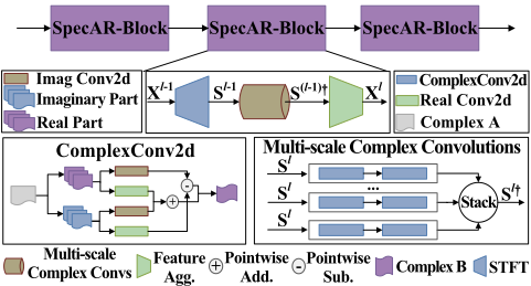
Where TFT(·) : RT →RT×F denotes a dimension/channelparallel time-frequency operator, which can be fulfilled by STFT (by default in this paper) or Wavelet Transform (WT). And MS-Conv† (·) denotes the parallel-computed complex convolutions with different dilation rates (sampling rates) in time-frequency receptive field of Sl-1 . Assume we have K different convolution blocks, then the output tensor will be in the form of S(l-1)† ∈ CM×T×F×K . More details of TFT(·) and MS-Conv† (·) are in Sec. 3.2 and 3.3.
Finally, for the feature aggregation stage, a block-wise average pooling is first conducted to compress the stacked feature tensor, S(l-1)† obtained fromMS-Conv† (·). Then a linear projection is used to transform the complex compressed features as real ones. This stage can be formalized as
Where, Avg Blk (·) : CK → C denotes the block-wise average pooling, Re/Im[·] is the element-wise real/complex part extractor, and Linear(·) denotes the complex-to-real linear projection. To further utilize the advantage of the skip connection, the fused time-frequency features, Xl† ∈ RM×T×F will be average-pooled along the frequency domain and transposed to get the shape-compatible output tensor in RT×M .
3.2 Time-Frequency Transformation
In order to decouple and analyze the periodic characteristics of time series while maintaining its temporal structure, we incorporate TFT in our SpecAR-Block. TFT can be fulfilled by the classic STFT or WT, which facilitates more efficient joint extraction of time-frequency features using 2D convolutions in subsequent learning stages. Following simplicity design principle, we use STFT by default. Fig. 2 illustrates the process of TFT for a given time series sample in an intuitive way.
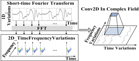
Following the symbol definition above, for each channel of the given input sequence Xl ∈ RT×M for l + 1-th SpecARBlock, the TFT calculation is formalized as
where Slm ∈ CT×F is the discrete STFT results, i.e., spectrogram of m-th channel input sequence Xlm ∈ RT×1 . Both window size and number of sample points for FFT are 2n+1, the hop length is set as 1, so that the input and output can have the same time length. The commonly used Hamming window function h(t) = 0.54 - 0.46 cos ( πt n ) is employed to modulate the input sequence. Moreover, it is also used Hanning window, Rectangular window and Blackman window, etc.
After applying the TFT to the time series, the highly coupled pure time domain data is expanded into a time-frequency representation. This transformation will enable the subsequent feature learning part to more intuitively analyze the periodic components of the input sequence and their respective evolution trends on the time-frequency distribution. However, it should be noted that the spectrogram actually carries not only the amplitude but also the phase information in each time-frequency unit, these are retained in the complex numbers. Hence, to fully utilize those contents, special treatment should be taken into consideration in the subsequent learning stage, which is discussed in the following section. Beyond that, as a crucial role in accurately representing frequencydomain features, window length determines the frequency resolution of the resulting spectrogram. Therefore, the effect of window length is also investigated in the experiments.
3.3 Multi-Scale Complex Convolutions
To make full use of the information in the spectrogram representation, i.e., the phase and the amplitude, the complex convolutions are utilized in SpecAR-Net. In addition, multiscale kernels for parallel convolutions are introduced to alleviate the contradiction of time-frequency resolution of TFT.
In order to avoid introducing more learning parameters, we use different dilation rates to achieve multi-scale feature extraction. Then the small network is designed to be constructed with K complex convolution blocks with different dilation rates but the same kernel size, 3 × 3. Given the input timefrequency tensor of l-th SpecAR-Block, Sl ∈ CM×T×F , The forward computation process can be roughly expressed as
Where Conv†k (·; d[k]) : CM → CM denotes the k-th convolution block with dilation rate of d[k] = 2k + 1. The specific calculation process for each Conv†k is as follows: assuming a complex convolution kernel w = (a + j ⊙ b) , and a complex input tensor h = (c + j ⊙ d), the complex convolution process, denoted as follows:
Finally, the ouput tensors of all the complex convolution blocks will be stacked together in block-wise to form the multi-scale feature tensor Sl† ∈ CM×T×F×K .
3.4 Temporal Order Preserving
To capture the global trend patterns of the input time series, the temporal order preserving (TOP) constraint is incorporated into our SpecAR-Net. This constraint is achieved by adding an order regression loss term on the basis of the original prediction loss. In practice, we use a temporal-shared learning function to construct such TOP loss term.
Given the final embeddings of SpecAR-Net, X∗ ∈ RT×M for an input sequence. The learning function Φ(·; u) : RM → R will encode each X∗ [t] as follows:
Where u is the temporal-shared learning parameters and t = 1, . . . , T is the time index of X∗ [t]. Based on this order regression mechanism, the TOP loss term for the current input sequence can be formalized as
Where LTOP denotes the TOP loss term, λ is the order regression penalty factor. And R(u) is the regularization term for loss LTOP, which can be written as the L1 or L2 norm of u, and we choose L2 in practice, i.e., R(u) = 12 ∥u∥22 . The loss can be expressed as the weighted summation of LTOP and the original loss for the current learning task, e.g., mean square error for forecasting or cross-entropy for classification.
4 Experiments
To verify the effectiveness and superiority of SpecAR-Net, a comprehensive set of experiments is conducted over 5 mainstream tasks, i.e., classification, anomaly detection, long-term forecasting, short-term forecasting and imputation. The benchmark datasets and corresponding experimental configurations are shown in Tab. 1. The backbones of the compared state-of-the-art (SoTA) models including RNNs (LSTM, LSTNet, LSSL), CNNs (TCN, TimesNet), MLPs (LightTS, DLinear) and Transformers (Autoformer [Wu et al., 2021], FEDformer, Informer, Reformer [Nikita Kitaev and Levskaya, 2020], Pyraformer [Liu et al., 2022a], ETSformer, Non-stationary Transformer [Liu et al., 2022b]). Furthermore, for specific tasks, cutting-edge models are also mentioned in the SoTA comparison this experiment. Specifically, N-HiTS [Challu et al., 2023] and N-BEATS [Oreshkin et al., 2019] are compared in short-term forecasting. Transformer [Xu et al., 2022] is selected for comparison in anomaly detection. For classification, Rocket [Dempster et al., 2020] and Flowformer [Wu et al., 2022] are compared.
4.1 Results onMainstreamTasks
Compared to other baseline methods, SpecAR-Net has achieved the best performance across all 5 tasks, as shown in Tab. 2 (where red and blue font denotes the best and secondbest results, respectively. ∗ in the Transformers indicates the name of ∗former.). Additionally, the results further validate the good generalization ability of SpecAR-Net, which can be regarded as a unified framework in time series analysis.
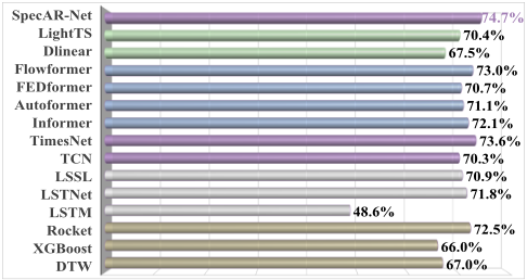
Classification (CLA) task can intuitively show the performance of our method in terms of high-level semantic representation of time series. The data used in this experiment is sourced from the UAE dataset (10 subsets) [Bagnall et al., 2018], comprising ten sub-datasets that encompass practical tasks such as gesture recognition, action recognition, audio recognition, and medical diagnosis. As shown in Fig. 3, SpecAR-Net has achieved remarkable results in classification task, with an average classification accuracy of 74.7%, surpassing other SoTA methods such as TimesNet (73.6%) and Flowformer (73%). It is worth noting that, compared to SpecAR-Net, TimesNet exhibits lower classification accuracy on most datasets, with an average accuracy reduction of 1.1%. Feature extraction can be conducted simultaneously in both time- and frequency-domains by SpecAR-Net, facilitating the capture of higher-level semantic representations.
Anomaly Detection (AD) plays a vital role in ensuring the orderly and secure operation of industrial production. However, anomaly detection often requires capturing exceptional signal within big data, which can easily get overwhelmed, making the detection task highly challenging. To fully validate the performance is such task, 5 widely-used datasets are employed, i.e., SMD [Su et al., 2019], MSL and SMAP [Hundman et al., 2018], SWaT [Mathur and Tippenhauer,
2016], and PSM [Abdulaal et al., 2021]. These datasets cover various real-world industrial applications, including service monitoring, spatial and earth sensing, and water treatment. The results are presented in Tab. 3. It is evident that our method achieved the optimal performance in the anomaly detection task, outperforming other comparative methods. The advanced Transformer-based approaches, FEDformer and Autoformer, have also both achieved good performance (84.97% and 84.26%). Frequency-domain information is introduced into the attention mechanism of both models, further highlighting the effectiveness of such information in time series representation. Comparatively, our method enables the joint extraction of deep-level time-frequency features from both the time- and frequency-domains, thereby facilitating the capture of abnormal patterns existing in time series.
Forecasting. In the long-term forecasting (LF) task, a set of benchmark datasets were utilized, including ETT [Zhou et al., 2021b], Electricity, Traffic, Weather, ExchangeRate [Lai et al., 2018a] and ILI (see download links in Appendix), which cover the application demands of 5 major real-world scenarios. Each dataset contains a segment of continuous time series, and sample data are obtained from these datasets using a sliding window approach. In the experiments, the input past length was set to 96, with ILL for 36. The prediction lengths is [96, 192, 336, 720], with ILI for [24, 36, 48, 60]. In the short-term forecasting (SF) task, we utilized the M4 dataset [Makridakis et al., 2018], which comprises 100,000 time series . These data were collected at different sampling rates, including yearly, quarterly, monthly, weekly, daily, and hourly intervals, covering a wide range of domains such as finance, industry, and demographics. For our experiments, the prediction sequence lengths is [6, 8, 13, 16, 24, 48]. Especially, all the results are averaged from four different prediction lengths for long-term forecasting, the results of shortterm forecasting tasks are calculated as weighted averages from multiple datasets with varying sample intervals. The experiments are conducted in two rounds in total. In the first round, MSE is used as loss function, and it achieved good results in both short-term and long-term forecasting tasks, although it did not reach the optimal level. See Tab.7 and 9 in Appendix for more details. In the second round, SpecAR-Net was conducted by introducing a order-preserving into the loss function. As shown in Tab. 4 and 5, our method achieves the best performance in both long- and short-term forecasting, indicating a positive role of the "order" information in time series forecasting. The order-preserving is equivalent to using the "order" information as prior knowledge to constrain the learning process of the model and compensate for the lost "order" information during feature extraction, ensuring that the model output possess a certain degree of sequentiality. Meanwhile, it also shows that our method is highly scalable.
Imputation (IMP) task relies on historical data to recover the missing data. This technique serves as the foundation of big data analytics, ensuring the temporal and spatial integrity of time series, thus supporting various subsequent tasks such as forecasting, classification, and anomaly detection. This experiment was conducted on 6 benchmark datasets, including ETT (4 subsets), Electricity and Weather. Random masking with masking rates of [12.5%, 25%, 37.5%, 50%] was used to simulate missing values. The experiment was conducted in two rounds. The first round of the experiment was conducted without order-preserving. And SpecAR-Net exhibits consistent performance with TimesNet, which is the best-performing method among the comparison methods. See Tab.11 in Appendix for more details. Tab. 6 presents the experimental results (average from 4 different mask ratios) after incorporating order-preserving, where SpecARNet achieves the best performance. This indicates that the monotonicity constraint is beneficial for capturing the global trend patterns in time series. Moreover, it also suggests that SpecAR-Net possesses strong capabilities in extracting timeand frequency-varying patterns.
| No. | Tasks | Datasets | Metrics | Series Length |
|---|---|---|---|---|
| 1 | Forecasting | Long-term: ETT(4subsets), ILI, Weather, Exchange, Electricity | MSE, MAE | 6∼720 (ILI:24∼60) |
| Short-term:M4(6 subsets) | SMAPE, MASE, OWA | 6∼48 | ||
| 2 | Imputation | ETT, Electricity, Weather | MSE, MAE | 96 |
| 3 | Classification | UEA(10 subsets) | Accuracy | 29∼1751 |
| 4 | Anomaly Detection | SMD, MSL, SMAP, SWaT, PSM | Precision, Recall, F1-Socre | 100 |
| Models | SpecAR-Net (ours) | TimesNet (2023) | Dlinear (2023) | ETS∗ (2022) | LightTS (2022) | Stationary (2022) | FED∗ (2022) | In∗ (2021) | Auto∗ (2021) |
|---|---|---|---|---|---|---|---|---|---|
| CLA(Accuracy) | 74.7 | 73.6 | 67.50 | 71.0 | 70.4 | 72.7 | 70.7 | 72.1 | 71.1 |
| AD(F1-Scores) | 86.45 | 86.34 | 82.46 | 82.87 | 84.23 | 82.08 | 84.97 | 78.83 | 84.26 |
| SF(OWA) | 0.850 | 0.851 | 1.051 | 1.172 | 1.051 | 0.930 | 0.918 | 1.230 | 0.939 |
| LF(MSE)(ILL) | 2.051 | 2.139 | 2.616 | 2.497 | 7.382 | 2.077 | 2.847 | 5.137 | 3.006 |
| IMP(MSE)(ETTh1) | 0.071 | 0.078 | 0.201 | 0.202 | 0.284 | 0.094 | 0.117 | 0.161 | 0.103 |
| Models | SpecAR-Net (ours) | TimesNet (ResNeXt) | TimesNet (Inception) | ETS∗ (2022) | LightTS (2022) | Stationary (2022a) | FED∗ (2022) | Dlinear (2023) | Auto∗ (2021) | In∗ (2021) |
|---|---|---|---|---|---|---|---|---|---|---|
| SMD | 86.55 | 85.81 | 85.12 | 83.13 | 82.53 | 84.62 | 85.08 | 77.10 | 85.11 | 81.65 |
| MSL | 81.72 | 85.15 | 84.18 | 85.03 | 78.95 | 77.5 | 78.57 | 84.88 | 79.05 | 84.06 |
| SMAP | 73.28 | 71.52 | 70.85 | 69.50 | 69.21 | 71.09 | 70.76 | 69.26 | 71.12 | 69.92 |
| SWaT | 93.42 | 91.74 | 92.10 | 84.91 | 93.33 | 79.88 | 93.19 | 87.52 | 92.74 | 81.43 |
| PSM | 97.28 | 97.47 | 95.21 | 91.76 | 97.15 | 97.29 | 97.23 | 93.55 | 93.29 | 77.10 |
| Avg F1 | 86.45 | 86.34 | 85.49 | 82.87 | 84.23 | 82.08 | 84.97 | 82.46 | 84.26 | 78.83 |
| Models | SpecAR-Net (ours) | TimesNet (2023) | N-HiTS (2022) | N-BEATS (2019) | ETS∗ (2022) | LightTS (2022) | Dlinear (2023) | FED∗ (2022) | Stationary (2022a) | Auto∗ (2021) |
|---|---|---|---|---|---|---|---|---|---|---|
| SMAPE | 11.844 | 11.829 | 11.927 | 11.851 | 14.718 | 13.525 | 13.639 | 12.840 | 12.780 | 12.909 |
| MASE | 1.582 | 1.585 | 1.613 | 1.599 | 2.408 | 2.111 | 2.095 | 1.701 | 1.756 | 1.771 |
| OWA | 0.850 | 0.851 | 0.861 | 0.855 | 1.172 | 1.051 | 1.051 | 0.918 | 0.930 | 0.939 |
4.2 Detailed Analysis
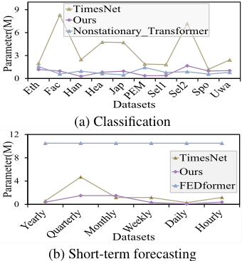
Model Complexity & Performance. To further analyze the performance of SpecAR-Net in the representation of time series, we selected comparable models with better performance in classification and forecasting tasks for model complexity analysis. Results in Fig. 4.2 show that better performance can be obtained by our method in the condition of less learnable parameters. This further illustrates the superiority of the proposed time-frequency joint learning mechanism.
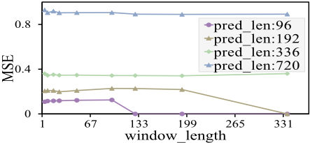
Effects of TF Resolution. The window length directly affects the time- and frequency-resolution of STFT, which reflect the richness of information in the time and frequency domains, which has a significant impact on extracting timefrequency variation. Therefore, in this experiment, different window lengths of [4, 8, 16, 24, 48, 96, 192, 336] were selected to investigate their effects on the model performance. Fig. 5 demonstrates that SpecAR-Net achieves optimal performance when the prediction lengths are [96, 192, 336, 720], corresponding to window lengths with [4, 24, 192, 192]. This finding indicates that the requirements for time-frequency resolution vary across different temporal analysis tasks, suggesting a varying dependency on both time- and frequencyfeatures. According to the Heisenberg uncertainty principle [Mallet and others, 1999], it is impossible for the timeand frequency-resolution to simultaneously reach their optimal values. In order to ensure that our model has good time series representation capability while maintaining a suitable computational complexity, window lengths are set as [8, 16, 24] in this paper.
| Models | SpecAR-Net (ours) | TimesNet (2023) | ETS∗ (2022) | LightTS (2022) | Dlinear (2023) | FED∗ (2022) | ||||||
|---|---|---|---|---|---|---|---|---|---|---|---|---|
| Metrics | MSE | MAE | MSE | MAE | MSE | MAE | MSE | MAE | MSE | MAE | MSE | MAE |
| ETTm1 | 0.398 | 0.407 | 0.400 | 0.406 | 0.429 | 0.425 | 0.435 | 0.437 | 0.403 | 0.407 | 0.448 | 0.452 |
| ETTm2 | 0.291 | 0.332 | 0.291 | 0.333 | 0.293 | 0.342 | 0.409 | 0.436 | 0.35 | 0.401 | 0.305 | 0.349 |
| ETTh1 | 0.458 | 0.455 | 0.458 | 0.450 | 0.542 | 0.510 | 0.491 | 0.479 | 0.456 | 0.452 | 0.440 | 0.460 |
| ETTh2 | 0.416 | 0.427 | 0.414 | 0.427 | 0.439 | 0.452 | 0.602 | 0.543 | 0.559 | 0.515 | 0.437 | 0.449 |
| Eelctricity | 0.192 | 0.294 | 0.192 | 0.295 | 0.208 | 0.323 | 0.229 | 0.329 | 0.212 | 0.300 | 0.214 | 0.327 |
| Traffic | 0.625 | 0.335 | 0.620 | 0.336 | 0.621 | 0.396 | 0.622 | 0.392 | 0.625 | 0.383 | 0.610 | 0.376 |
| Weather | 0.257 | 0.284 | 0.259 | 0.287 | 0.271 | 0.334 | 0.261 | 0.312 | 0.265 | 0.317 | 0.309 | 0.360 |
| ExchangeRate | 0.384 | 0.425 | 0.416 | 0.443 | 0.410 | 0.427 | 0.385 | 0.447 | 0.354 | 0.414 | 0.519 | 0.500 |
| ILL | 2.051 | 0.903 | 2.139 | 0.931 | 2.497 | 1.004 | 7.382 | 2.003 | 2.616 | 1.090 | 2.847 | 1.144 |
| Models | SpecAR-Net (ours) | TimesNet (2023) | ETS. (2022) | LightTS (2022) | DLinear (2023) | FED∗ (2022) | ||||||
|---|---|---|---|---|---|---|---|---|---|---|---|---|
| Metrics | MSE | MAE | MSE | MAE | MSE | MAE | MSE | MAE | MSE | MAE | MSE | MAE |
| ETTm1 | 0.026 | 0.105 | 0.027 | 0.107 | 0.120 | 0.253 | 0.104 | 0.218 | 0.093 | 0.206 | 0.062 | 0.177 |
| ETTm2 | 0.021 | 0.087 | 0.022 | 0.089 | 0.208 | 0.327 | 0.046 | 0.151 | 0.096 | 0.208 | 0.101 | 0.215 |
| ETTh1 | 0.071 | 0.178 | 0.078 | 0.187 | 0.202 | 0.329 | 0.284 | 0.373 | 0.201 | 0.306 | 0.117 | 0.246 |
| ETTh2 | 0.046 | 0.141 | 0.049 | 0.146 | 0.367 | 0.436 | 0.119 | 0.250 | 0.142 | 0.259 | 0.163 | 0.279 |
| Electricity | 0.092 | 0.210 | 0.092 | 0.210 | 0.214 | 0.339 | 0.131 | 0.262 | 0.132 | 0.260 | 0.130 | 0.259 |
| Weather | 0.031 | 0.057 | 0.030 | 0.054 | 0.076 | 0.171 | 0.055 | 0.117 | 0.052 | 0.110 | 0.099 | 0.203 |
5 Conclusions
SpecAR-Net can be used as a universal foundational model for time-frequency representation and analysis of time series. Through the time-frequency transformation, SpecARNet overcomes the limitations of semantic representation in 1D time series caused by the coupling of multiple components such as trending, periodicity, and abruptness. This facilitates the simultaneous extraction and fusion of timefrequency variation patterns from a 2D space. Experimental results demonstrate that SpecAR-Net achieves optimal performance in 5 tasks, including classification, anomaly detection, imputation, long- and short-term forecasting.
Acknowledgements
This work is supported by National Natural Science Foundation of China (No. 62206258).
Contribution Statement
Yi Dong∗ , Liwen Zhang∗ and Youcheng Zhang∗ are authors of equal contributions: Yi contributed code implementation, experimental operation and the draft of the paper; Liwen contributed idea, algorithm design, and writing of introduction, method and rebuttal; Youcheng contributed experiment design, paper structure and paper polishing. Zhe Ma† is the corresponding author.
@inproceedings{ijcai2024p433,
  title     = {SpecAR-Net: Spectrogram Analysis and Representation Network for Time Series},
  author    = {Dong, Yi and Zhang, Liwen and Zhang, Youcheng and Peng, Shi and Chen, Wen and Ma, Zhe},
  booktitle = {Proceedings of the Thirty-Third International Joint Conference on
               Artificial Intelligence, {IJCAI-24}},
  publisher = {International Joint Conferences on Artificial Intelligence Organization},
  editor    = {Kate Larson},
  pages     = {3917--3925},
  year      = {2024},
  month     = {8},
  note      = {Main Track},
  doi       = {10.24963/ijcai.2024/433},
  url       = {https://doi.org/10.24963/ijcai.2024/433},
}
TY - CPAPER TI - SpecAR-Net: Spectrogram Analysis and Representation Network for Time Series AU - Dong, Yi AU - Zhang, Liwen AU - Zhang, Youcheng AU - Peng, Shi AU - Chen, Wen AU - Ma, Zhe T2 - Proceedings of the Thirty-Third International Joint Conference on Artificial Intelligence, IJCAI-24 PB - International Joint Conferences on Artificial Intelligence Organization PY - 2024 SP - 3917 EP - 3925 DO - 10.24963/ijcai.2024/433 UR - https://doi.org/10.24963/ijcai.2024/433 ER -Copied
Machine-readable versions of this paper, for tools and AI agents:





