
Deep Frequency Derivative Learning for Non-stationary Time Series Forecasting
Proceedings of the Thirty-Third International Joint Conference on Artificial Intelligence. Main Track. Pages 3944-3952.
https://doi.org/10.24963/ijcai.2024/436
Keywords
- Data Mining: DM: Mining spatial and/or temporal data
- Machine Learning: ML: Time series and data streams
Abstract
While most time series are non-stationary, it is inevitable for models to face the distribution shift issue in time series forecasting. Existing solutions manipulate statistical measures (usually mean and std.) to adjust time series distribution. However, these operations can be theoretically seen as the transformation towards zero frequency component of the spectrum which cannot reveal full distribution information and would further lead to information utilization bottleneck in normalization, thus hindering forecasting performance. To address this problem, we propose to utilize the whole frequency spectrum to transform time series to make full use of data distribution from the frequency perspective. We present a deep frequency derivative learning framework, DERITS, for non-stationary time series forecasting. Specifically, DERITS is built upon a novel reversible transformation, namely Frequency Derivative Transformation (FDT) that makes signals derived in the frequency domain to acquire more stationary frequency representations. Then, we propose the Order-adaptive Fourier Convolution Network to conduct adaptive frequency filtering and learning. Furthermore, we organize DERITS as a parallel-stacked architecture for the multi-order derivation and fusion for forecasting. Finally, we conduct extensive experiments on several datasets which show the consistent superiority in both time series forecasting and shift alleviation.
- Models LTSF-Linear +RevIN +Dish-TS +FDT Metrics MAE RMSE MAE RMSE MAE RMSE MAE RMSE Exchange 96 0.038 0.052 0.040 0.055 0.039 0.053 0.036 0.050 192 0.053 0.069 0.052 0.070 0.055 0.071 0.050 0.068 336 0.064 0.085 0.069 0.094 0.068 0.090 0.060 0.082 720 0.092 0.116 0.115 0.145 0.110 0.132 0.090 0.114 Weather 96 0.040 0.081 0.042 0.085 0.039 0.082 0.037 0.080 192 0.048 0.089 0.045 0.089 0.046 0.090 0.043 0.088 336 0.056 0.098 0.053 0.097 0.055 0.099 0.050 0.095 720 0.065 0.106 0.061 0.108 0.060 0.105 0.056 0.103 ILI 24 0.167 0.214 0.151 0.199 0.156 0.203 0.141 0.196 36 0.179 0.231 0.168 0.228 0.171 0.230 0.158 0.212 48 0.165 0.216 0.158 0.214 0.160 0.214 0.151 0.198 60 0.166 0.212 0.161 0.204 0.164 0.210 0.152 0.196 Electricity 96 0.045 0.075 0.046 0.078 0.044 0.074 0.041 0.072 192 0.043 0.070 0.042 0.070 0.043 0.071 0.040 0.068 336 0.044 0.071 0.043 0.070 0.042 0.070 0.040 0.067 720 0.054 0.080 0.048 0.076 0.050 0.077 0.048 0.076 ETTm1 96 0.055 0.080 0.054 0.078 0.052 0.077 0.051 0.072 192 0.060 0.087 0.058 0.086 0.057 0.085 0.056 0.084 336 0.065 0.093 0.062 0.090 0.064 0.092 0.060 0.088 720 0.072 0.099 0.070 0.100 0.071 0.102 0.066 0.093
- [Ariyo et al., 2014] Adebiyi A Ariyo, Adewumi O Adewumi, and Charles K Ayo. Stock price predic- tion using the arima model. In 2014 UKSim-AMSS 16th international conference on computer modelling and simulation, pages 106-112. IEEE, 2014.
- [Asuncion and Newman, 2007] Arthur Asuncion and David Newman. Uci machine learning repository, 2007.
- [Bai et al., 2018] Shaojie Bai, J. Zico Kolter, and Vladlen Koltun. An empirical evaluation of generic convolutional and recurrent networks for sequence modeling. CoRR, abs/1803.01271, 2018.
- [Ben-Akiva et al., 1998] Moshe Ben-Akiva, Michel Bier- laire, Haris Koutsopoulos, and Rabi Mishalani. Dynamit: a simulation-based system for traffic prediction. In DAC- CORD short term forecasting workshop, volume 12. Delft The Netherlands, 1998.
- [Brockwell and Davis, 2009] Peter J Brockwell and Richard A Davis. Time series: theory and methods. Springer science & business media, 2009.
- [Cao et al., 2020] Defu Cao, Yujing Wang, Juanyong Duan, Ce Zhang, Xia Zhu, Congrui Huang, Yunhai Tong, Bix- iong Xu, Jing Bai, Jie Tong, and Qi Zhang. Spectral temporal graph neural network for multivariate time-series forecasting. In NeurIPS, 2020.
- [Deb et al., 2017] Chirag Deb, Fan Zhang, Junjing Yang, Siew Eang Lee, and Kwok Wei Shah. A review on time se- ries forecasting techniques for building energy consump- tion. Renewable and Sustainable Energy Reviews, 74:902- 924, 2017.
- [Fan et al., 2022] Wei Fan, Shun Zheng, Xiaohan Yi, Wei Cao, Yanjie Fu, Jiang Bian, and Tie-Yan Liu. DEPTS: deep expansion learning for periodic time series forecast- ing. In ICLR. OpenReview.net, 2022.
- [Fan et al., 2023] Wei Fan, Pengyang Wang, Dongkun Wang, Dongjie Wang, Yuanchun Zhou, and Yanjie Fu. Dish-ts: a general paradigm for alleviating distribution shift in time series forecasting. In Proceedings of the AAAI Conference on Artificial Intelligence, volume 37, pages 7522-7529, 2023.
- [Hirsa and Neftci, 2013] Ali Hirsa and Salih N Neftci. An introduction to the mathematics of financial derivatives. Academic press, 2013.
- [Holt, 1957] Charles C Holt. Forecasting trends and seasonal by exponentially weighted moving averages. ONR Memo- randum, 52(2), 1957.
- [Huang et al., 1998] Norden E Huang, Zheng Shen, Steven R Long, Manli C Wu, Hsing H Shih, Quanan Zheng, Nai-Chyuan Yen, Chi Chao Tung, and Henry H Liu. The empirical mode decomposition and the hilbert spectrum for nonlinear and non-stationary time series analysis. Proceedings of the Royal Society of London. Se- ries A: mathematical, physical and engineering sciences, 454(1971):903-995, 1998.
- [Katznelson, 1970] Y. Katznelson. An introduction to har- monic analysis. Cambridge University Press,, 1970.
- [Kim et al., 2022] Taesung Kim, Jinhee Kim, Yunwon Tae, Cheonbok Park, Jang-Ho Choi, and Jaegul Choo. Re- versible instance normalization for accurate time-series forecasting against distribution shift. In International Con- ference on Learning Representations, 2022.
- [King, 1966] Benjamin F King. Market and industry fac- tors in stock price behavior. the Journal of Business, 39(1):139-190, 1966.
- [Lai et al., 2018] Guokun Lai, Wei-Cheng Chang, Yiming Yang, and Hanxiao Liu. Modeling long-and short-term temporal patterns with deep neural networks. In SIGIR, pages 95-104, 2018.
- [Liu et al., 2022a] Minhao Liu, Ailing Zeng, Muxi Chen, Zhijian Xu, Qiuxia Lai, Lingna Ma, and Qiang Xu. Scinet: time series modeling and forecasting with sample convo- lution and interaction. Advances in Neural Information Processing Systems, 35:5816-5828, 2022.
- [Liu et al., 2022b] Yong Liu, Haixu Wu, Jianmin Wang, and Mingsheng Long. Non-stationary transformers: Explor- ing the stationarity in time series forecasting. Advances in Neural Information Processing Systems, 35:9881-9893, 2022.
- [Liu et al., 2023] Zhiding Liu, Mingyue Cheng, Zhi Li, Zhenya Huang, Qi Liu, Yanhu Xie, and Enhong Chen. Adaptive normalization for non-stationary time series forecasting: A temporal slice perspective. In Thirty- seventh Conference on Neural Information Processing Systems, 2023.
- [Lorenz, 1956] Edward N Lorenz. Empirical orthogonal functions and statistical weather prediction, volume 1. Massachusetts Institute of Technology, Department of Me- teorology Cambridge, 1956.
- [Nie et al., 2023] Yuqi Nie, Nam H. Nguyen, Phanwadee Sinthong, and Jayant Kalagnanam. A time series is worth 64 words: Long-term forecasting with transformers. In International Conference on Learning Representations, 2023.
- [Nussbaumer and Nussbaumer, 1982] Henri J Nussbaumer and Henri J Nussbaumer. The fast Fourier transform. Springer, 1982.
- [Ogasawara et al., 2010] Eduardo Ogasawara, Leonardo C Martinez, Daniel De Oliveira, Geraldo Zimbrão, Gisele L Pappa, and Marta Mattoso. Adaptive normalization: A novel data normalization approach for non-stationary time series. In The 2010 International Joint Conference on Neu- ral Networks (IJCNN), pages 1-8. IEEE, 2010.
- [Oreshkin et al., 2019] Boris N Oreshkin, Dmitri Carpov, Nicolas Chapados, and Yoshua Bengio. N-beats: Neural basis expansion analysis for interpretable time series fore- casting. arXiv preprint arXiv:1905.10437, 2019.
- [Oreshkin et al., 2020] Boris N. Oreshkin, Dmitri Carpov, Nicolas Chapados, and Yoshua Bengio. N-beats: Neural basis expansion analysis for interpretable time series fore- casting. In International Conference on Learning Repre- sentations, 2020.
- [Paszke et al., 2019] Adam Paszke, Sam Gross, Francisco Massa, Adam Lerer, James Bradbury, Gregory Chanan, Trevor Killeen, Zeming Lin, Natalia Gimelshein, Luca Antiga, Alban Desmaison, Andreas Köpf, Edward Z. Yang, Zachary DeVito, Martin Raison, Alykhan Tejani, Sasank Chilamkurthy, Benoit Steiner, Lu Fang, Junjie Bai, and Soumith Chintala. Pytorch: An imperative style, high- performance deep learning library. In NeurIPS, pages 8024-8035, 2019.
- [Priestley and Rao, 1969] MB Priestley and T Subba Rao. A test for non-stationarity of time-series. Journal of the Royal Statistical Society Series B: Statistical Methodol- ogy, 31(1):140-149, 1969.
- [Salinas et al., 2020] David Salinas, Valentin Flunkert, Jan Gasthaus, and Tim Januschowski. Deepar: Probabilistic forecasting with autoregressive recurrent networks. Inter- national Journal of Forecasting, 36(3):1181-1191, 2020.
- [Vaswani et al., 2017] Ashish Vaswani, Noam Shazeer, Niki Parmar, Jakob Uszkoreit, Llion Jones, Aidan N Gomez, Łukasz Kaiser, and Illia Polosukhin. Attention is all you need. In Advances in neural information processing sys- tems, pages 5998-6008, 2017.
- [Whittle, 1951] Peter Whittle. Hypothesis testing in time se- ries analysis. Almqvist & Wiksells boktr., 1951.
- [Whittle, 1963] Peter Whittle. Prediction and regulation by linear least-square methods. English Universities Press, 1963.
- [Wiles et al., 2021] Olivia Wiles, Sven Gowal, Florian Stim- berg, Sylvestre Alvise-Rebuffi, Ira Ktena, Krishnamurthy Dvijotham, and Taylan Cemgil. A fine-grained analysis on distribution shift. arXiv preprint arXiv:2110.11328, 2021.
- [Woo et al., 2022a] Gerald Woo, Chenghao Liu, Doyen Sa- hoo, Akshat Kumar, and Steven Hoi. Deeptime: Deep time-index meta-learning for non-stationary time-series forecasting. arXiv preprint arXiv:2207.06046, 2022.
- [Woo et al., 2022b] Gerald Woo, Chenghao Liu, Doyen Sa- hoo, Akshat Kumar, and Steven C. H. Hoi. Cost: Con- trastive learning of disentangled seasonal-trend represen- tations for time series forecasting. In ICLR. OpenRe- view.net, 2022.
- [Wu et al., 2021] Haixu Wu, Jiehui Xu, Jianmin Wang, and Mingsheng Long. Autoformer: Decomposition transform- ers with auto-correlation for long-term series forecasting. In NeurIPS, pages 22419-22430, 2021.
- [Yi et al., 2023a] Kun Yi, Qi Zhang, Longbing Cao, Shoujin Wang, Guodong Long, Liang Hu, Hui He, Zhendong Niu, Wei Fan, and Hui Xiong. A survey on deep learning based time series analysis with frequency transformation. arXiv preprint arXiv:2302.02173, 2023.
- [Yi et al., 2023b] Kun Yi, Qi Zhang, Wei Fan, Shoujin Wang, Pengyang Wang, Hui He, Ning An, Defu Lian, Longbing Cao, and Zhendong Niu. Frequency-domain MLPs are more effective learners in time series forecast- ing. In Thirty-seventh Conference on Neural Information Processing Systems, 2023.
- [Yi et al., 2024] Kun Yi, Qi Zhang, Wei Fan, Hui He, Liang Hu, Pengyang Wang, Ning An, Longbing Cao, and Zhen- dong Niu. Fouriergnn: Rethinking multivariate time series forecasting from a pure graph perspective. Advances in Neural Information Processing Systems, 36, 2024.
- [Zeng et al., 2023] Ailing Zeng, Muxi Chen, Lei Zhang, and Qiang Xu. Are transformers effective for time series fore- casting? In AAAI, pages 11121-11128. AAAI Press, 2023.
- [Zhang et al., 2017] Liheng Zhang, Charu C. Aggarwal, and Guo-Jun Qi. Stock price prediction via discovering multi- frequency trading patterns. In KDD, pages 2141-2149, 2017.
- [Zhou et al., 2021] Haoyi Zhou, Shanghang Zhang, Jieqi Peng, Shuai Zhang, Jianxin Li, Hui Xiong, and Wancai Zhang. Informer: Beyond efficient transformer for long sequence time-series forecasting. In Proceedings of AAAI, 2021.
- [Zhou et al., 2022] Tian Zhou, Ziqing Ma, Qingsong Wen, Xue Wang, Liang Sun, and Rong Jin. FEDformer: Fre- quency enhanced decomposed transformer for long-term series forecasting. In ICML, 2022.
References were extracted automatically from the PDF and may contain errors.
Full text extracted automatically from the PDF; figures, tables and equations may differ. The PDF is the version of record.
1 Introduction
Time series forecasting has been playing an important role in a variety of real-world industries, such as traffic analysis [Ben-Akiva et al., 1998], weather prediction [Lorenz, 1956], financial estimation [King, 1966; Ariyo et al., 2014], energy planning [Deb et al., 2017], etc. Following by classic statistical methods (e.g., ARIMA [Whittle, 1963]), many
* Corresponding Author.
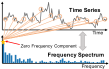
- (a) Transformation with only the zero frequency component.
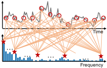
Figure 1: Given one time series and its frequency spectrum, the main comparison between existing works (a) and our method (b).
deep machine learning-based time series forecasting methods [Salinas et al., 2020; Oreshkin et al., 2019] have recently achieved superior performance in different scenarios. Despite the remarkable success, the non-stationarity widely existing in time series data has still been a critical but under-addressed challenge for accurate forecasting [Priestley and Rao, 1969; Huang et al., 1998; Brockwell and Davis, 2009].
Since time series data are usually collected at a high frequency over a long duration, such non-stationary sequences with millions of timesteps inevitably let forecasting models face the distribution shifts over time. This would lead to performance degradation at test time [Kim et al., 2022] due to the covariate shift or the conditional shift [Woo et al., 2022a]. For this issue, pioneer works [Ogasawara et al., 2010] propose to normalize time series data with global statistics; one recent work [Kim et al., 2022] proposes to use instance statistics to normalize time series against distribution shifts. Then, some work brings statistical information into self-attention computation [Liu et al., 2022b]; another work [Fan et al., 2023] transform time series with learnable statistics and consider shifts input and output sequences, and [Liu et al., 2023] utilize predicted sliced statistics for adaptive normalization.
Most of these existing works focus on transforming each timestep of time series with certain statistics (usually mean and std.) After our careful theoretical analysis 1 , we have found that these operations can actually be regarded as the normalization towards the zero frequency component of the spectrum in the frequency domain, as shown in Figure 1(a). However, they cannot fully utilize distribution information of time series signals; moreover, this would lead to information utilization bottleneck in normalization and thus hinders the performance of time series forecasting. To address this problem, we propose to utilize the whole frequency spectrum for the transformation of time series, to make full use of distribution information of time series from the frequency perspective and in the meanwhile transform time series into more stationary space thus making more accurate forecasting. Figure 1(b) has shown our method with the whole frequency spectrum.
1 We leave the details of our theoretical analysis in Appendix B.1
Motivated by this view, we then present a deep frequency derivative learning framework, DERITS, for non-stationary time series forecasting. The core idea of DERITS lies in two folds: (i) employing the whole frequency spectrum to take the derivative of time series signals, and (ii) learning frequency dependencies on more stationary transformed representations. Specifically, we first propose a novel transformation for time series signals in DERITS, namely Frequency Derivative Transformation (FDT), which mainly includes two stages. In the first stage, the raw signals in the time domain are transformed into the frequency domain with Fourier transform [Nussbaumer and Nussbaumer, 1982] for further learning. In the second stage, the transformed frequency components are derived with respect to timestamps to get more stationary frequency representations. Inspired by the derivative in mathematics [Hirsa and Neftci, 2013], FDT let models aim for modeling gradients of signals rather than raw input signals, which could mitigate their burden of forecasting with distribution shifts by resolving non-stationary factors (e.g., the shift of trends) in the original time series through one- or high-order derivation.
After acquiring more stationary representations, we further propose a novel architecture, Order-adaptive Fourier Convolution Network (OFCN) in DERITS for the frequency filtering and dependency learning to accomplish the forecasting. Concretely, OFCN is composed of (i) Order-adaptive frequency filter that adaptively extracts meaningful patterns by excluding high-frequency noises for derived signals of different orders, and (ii) Fourier convolutions that conduct dependency mappings and learning for complex values in the frequency domain. Since OFCN is operating in the projection space by FDT, we thus utilize the inverse Frequency Derivative Transformation to recover the predicted frequency components back to the original time domain. Inspired by previous work [Kim et al., 2022], we let all stages of FDT fully reversible and symmetric and make OFCN predict in the more stationary frequency space, which reveals our superiority in enhancing forecasting against distribution shifts. Furthermore, in order for the multi-order derivative learning, we have organized DERITS as a parallel-stacked architecture to fuse representations of different orders. Specifically, DERITS is composed of several parallel branches, each of which represents an order of derivation and prediction corresponding for its FDT and OFCN. Note that the Fourier convolution adapted in each branch is not parameter-sharing and after the distinct processing of different branches, the outputs are fused to achieve the final time series forecasting. In summary, our main contribution can be listed as follows:
- Motivated by our theoretical analysis towards existing time series normalization techniques from the frequency spectrum perspective, we propose to utilize the whole frequency spectrum for the transformation of time series.
- We present a deep frequency derivative learning framework, namely DERITS, built upon our proposed Frequency Derivative Transformation (with its inverse) for non-stationary time series forecasting.
- We introduce the novel Order-adaptive Fourier Convolution Network, for the frequency dependency learning and organize DERITS as a parallel-stacked architecture to fuse multi-order representations for forecasting.
- We have conducted extensive experiments on seven realworld datasets, which have demonstrated the consistent superiority compared with state-of-the-art methods in both time series forecasting and shift alleviation.
2 RelatedWork
2.1 Time Series Forecasting with Non-stationarity
Time series forecasting is a longstanding research topic. Traditionally, researchers have proposed statistical approaches, including exponentially weighted moving averages [Holt, 1957] and ARMA [Whittle, 1951]. Recently, with the advanced development of deep learning, many deep time series forecasting methods have been developed, including RNN-based methods (e.g., deepAR [Salinas et al., 2020], LSTNet [Lai et al., 2018]), CNN-based methods (e.g., SCINet [Liu et al., 2022a], TCN [Bai et al., 2018]), MLP-based Methods (e.g., DLinear [Zeng et al., 2023], N-BEATS [Oreshkin et al., 2020]) and Transformer-based methods (e.g., Autoformer [Wu et al., 2021], PatchTST [Nie et al., 2023]). While time series are non-stationary, existing works try to normalize time series with global statistics [Ogasawara et al., 2010], instance statistics [Kim et al., 2022], learnable statistics [Fan et al., 2023] and sliced statistics [Liu et al., 2023] in order to relieve the influence of distribution shift on forecasting.
2.2 Frequency Analysis in Time Series Modeling
The frequency analysis has been widely used to extract knowledge of the frequency domain in time series modeling and forecasting [Yi et al., 2023a]. Specifically, SFM [Zhang et al., 2017] adopts Discrete Fourier Transform to decompose the hidden state of time series by LSTM into frequency components; StemGNN [Cao et al., 2020] adopts Graph Fourier Transform to perform graph convolutions and FourierGNN [Yi et al., 2024] uses Discrete Fourier Transform to computes series-wise correlations. Autoformer [Wu et al., 2021] replaces self-attention in Transformer [Vaswani et al., 2017] and proposes the auto-correlation mechanism implemented by Fast Fourier Transform. FEDformer [Zhou et al., 2022] introduces Discrete Fourier Transform-based frequency enhanced attention. DEPTS [Fan et al., 2022] utilizes Discrete Cosine Transform to extract periodic patterns. In addition, [Woo et al., 2022b] transforms hidden features of time series into the frequency domain with Discrete Fourier Transform to enhance the time series representation learning. [Yi et al., 2023b] combines Fast Fourier Transform with multi-layer perceptrons for time series forecasting.
3 ProblemFormulation
Time Series Forecasting Let x = [x1; x2; · · · ; xT ] ∈ RT×D be regularly sampled multi-variate time series with T timestamps and D variates, where xt ∈ RD denotes the multi-variate values at timestamp t. In the task of time series forecasting, we use Xt ∈ RL×D to denote the lookback window, a length-L segment of x ending at timestamp t (exclusive), namely Xt = xt-L:t = [xt-L; xt-L+1; · · · ; xt-1]. Similarly, we represent the horizon window as a length-H segment of x starting from timestamp t (inclusive) as Yt, so we have Yt = xt:t+H = [xt; xt+1; · · · ; xt+H-1]. The classic time series forecasting formulation is to project lookback values Xt into horizon values Yt. Specifically, a typical forecasting model Fθ : RL×D → RH×D produces forecasts by ˆYt = fθ(Xt) where ˆYt stands for the forecasting results and θ encapsulates the model parameters.
Non-stationarity and Distribution Shifts In this paper, we aim to study the problem of non-stationarity in deep time series forecasting. As aforementioned in Section 1, long time series with millions of timesteps let forecasting models face distribution shifts over time due to the nonstationarity. The distribution shifts in time series forecasting are usually the covariate shift [Wiles et al., 2021; Woo et al., 2022a]. Specifically, given a stochastic process, let p (xt, xt-1, . . . , xt-L+1) be the unconditional joint distribution of a length L segment where xt is the value of univariate time series at timestamp t. The stochastic process experiences covariate shift if any two segments are drawn from different distributions, i.e. p (xt-L, xt-L+1 . . . , xt-1) ̸= p (xt′-L, xt′-L+1, . . . , xt′-1) , ∀t ̸= t′ . Subsequently, let p (xt | xt-1, . . . , xt-L) represents the conditional distribution of xt, such a stochastic process experiences conditional shift if two segments have different conditional distributions, i.e. p (xt | xt-1, . . . , xt-L+1, xt-L) ̸= p (xt′ | xt′-1, . . . , xt′-L+1, xt′-L) , ∀t ̸= t′ .
4 Methodology
In this section, we elaborate on our proposed deep frequency derivative learning framework, DERITS, designed for nonstationary time series forecasting. First, we introduce our novel reversible transformation, Frequency Derivative Transformation (FDT) in Section 4.1. Then, to fuse multi-order information, we present the parallel-stacked frequency derivative learning architecture in Section 4.2. Finally, we introduce our Order-adaptive Fourier Convolution Network (OFCN) for frequency learning in Section 4.3.
4.1 Frequency Derivative Transformation
As aforementioned in Section 1, to fully utilize the whole frequency spectrum for the transformation of time series with sufficient distribution information, we propose the novel Frequency Derivative Transformation (FDT) to achieve more stationary frequency representations of time series signals. For this aim, FDT mainly includes two distinct stages respectively for domain transformation and frequency derivation.
Domain Transformation
In the first stage, to be specific, we make use of fast Fourier transform [Nussbaumer and Nussbaumer, 1982] to enable the decomposition of time series signals from the time domain into their inherent frequency components. Formally, given the time domain input signals X(t), we convert it into the frequency domain by:
where F is the fast Fourier transform, f is the frequency variable, t is the integral variable, and j is the imaginary unit, defined as the square root of -1; ∫ ∞ -∞ X(t) cos(2πf t)dt is the real part of X and is abbreviated as Re(X); ∫ ∞ -∞ X(t) sin(2πft)dt is the imaginary part and is abbreviated as Im(X). After that we can rewrite X as X = Re(X ) + jIm(X ).
Frequency Derivation
In the second stage, with the transformed frequency components, we propose to utilize the whole frequency spectrum for the signal derivation, in order to represent time series in a more stationary space. The basic idea is to perform our proposed Fourier Derivative Operator in the frequency domain, which is defined as follows:
Definition 1 (Fourier Derivative Operator). Given the time domain input signals X(t) and its corresponding frequency components X(f), we then define R(X(f)) := (j2πf)X(f) as the Fourier Derivative Operator (FDO), where f is the frequency variable and j is the imaginary unit.
In the derivation, different order usually represents different signal representations. We propose to incorporate multiorder information in DERITS to further enhance the forecasting. For this aim, we extend above definition and further define the k-order Fourier Derivative Operator Rk as:
With such two stages, we can finally write the k-order Frequency Derivation Transformation FDTk as:
where X(t) is the time domain input signal; F stands for fast Fourier transform and f is the frequency variable.
Proposition 1. Given X(t) in the time domain and X(f) in the frequency domain correspondingly, the k-order Fourier Derivative Operator on X (f ) is equivalent to k-order derivation on X(t) with respect to t in the time domain, written by:
where F is Fourier transform, dk dtk is k-order derivative with respect to t, and j is the imaginary unit.
We leave the detailed proof in Appendix B.2. With such a equivalence, we can find out FDT can actually achieve more stationary representations in the lower order by derivation. For example, the shifts caused by a single trend signal in time series can nearly degraded be zero. We include the specific analysis in Appendix D. Then, with less distribution shifts and non-stationarity by FDT, the deep networks can have large potential to perform more accurate forecasting.
4.2 Frequency Derivative Learning Architecture
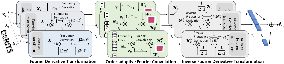
The main architecture of DERITS is depicted in Figure 2, which is built upon the Frequency Derivative Transformation and its inverse for the frequency derivative learning.
FDT/iFDT As mentioned in Section 4.1, DERITS needs to conduct predictions in a more stationary frequency space achieved by frequency derivative transformation. We naturally need to recover the predictions back to the time domain for final forecasting and evaluation. To make FDT fully reversible, we let both stages of FDT reversible, including Fourier transform and Fourier Derivation. Specifically, following Equation (3), we can symmetrically write the inverse frequency derivative transformation (iFDT) of k order as:
where R-1 k is the inverse process of Fourier Derivative Operator of k order; F -1 is the inverse Fourier transform; X(f) is the frequency components that need to be recovered to the time domain. Actually, the inverse process R-1 k is equivalent to an integration operator in the time domain. More details can be found in Appendix D.
The Parallel-Stacked Architecture
To conduct the multi-order frequency derivation transformation and learning, we have organized our DERITS framework as a parallel-stacked architecture, where each branch represents an order of frequency derivation learning, as shown in Figure 2. Let DERITS have K branches in total. For each branch, we first take lookback values Xt to frequency derivative transformation by:
where FDTk is the k-order FDT and X k t is the frequency derivative representation for Xkt at timestamp t. Then, the learned representations for each branch are taken to the Fourier Convolution Network (FCN) for frequency dependency learning. Since our FCN is order-adaptive in each parallel branch, we also take k as input with the computation by:
where Hk t are the predicted frequency components for X k t . Note that FourierConvolution is not parameter-sharing for different branches. After that, we recover the predictions to the time domain by:
where Hkt is the recovered representation of k order in the time domain. After acquiring it, we finally fuse the multiorder representations from parallel branches for the forecasting with MLP layers, which is given by:
where ˆYt are forecasting results by DERITS for evaluation.
4.3 Order-adaptive Fourier Convolution Network
Apart from the frequency derivative transformation, another aim of DERITS is to accomplish the dependency learning with the derived signals in the frequency domain. We thus introduce a novel network architecture, namely Orderadaptive Fourier Convolution Network (OFCN) to enable the frequency learning. Specifically, OFCN is composed of two important components, i.e., order-adaptive frequency filter and Fourier convolutions, which are illustrated as follows:
Order-adaptive Frequency Filter We aim to fuse multiorder derived signal information for forecasting, while it is notable that different order corresponds to different frequency comments. Since time series include not only meaningful patterns but also high-frequency noises, we develop an orderadaptive frequency filter to enhance the learning process.
Supposing there are S frequencies in X k t , we sort X k t on the frequencies in a descending order of amplitude for each frequency to get X ′kt for k order. Then, we design an adaptive mask mk to concentrate on only S 2(K-k) frequency components of X k t for further learning. We write the adaptive frequency filtering process by:
| Models Metrics | DERITS MAE RMSE | FreTS MAE RMSE | PatchTST MAE RMSE | LTSF-Linear MAE RMSE | FEDformer MAE RMSE | Autoformer MAE RMSE | Informer MAE RMSE | NSTransformer MAE RMSE | |||||||||
|---|---|---|---|---|---|---|---|---|---|---|---|---|---|---|---|---|---|
| Exchange | 96 192 336 720 | 0.035 0.050 0.060 0.086 | 0.050 0.066 0.083 0.108 | 0.037 0.050 0.062 0.088 | 0.051 0.067 0.082 0.110 | 0.039 0.055 0.071 0.132 | 0.052 0.074 0.093 0.166 | 0.038 0.053 0.064 0.092 | 0.052 0.069 0.080 0.116 | 0.050 0.060 0.070 0.142 | 0.067 0.080 0.095 0.174 | 0.054 0.065 0.085 0.150 | 0.070 0.083 0.101 0.181 | 0.066 0.068 0.093 0.117 | 0.084 0.088 0.127 0.170 | 0.052 0.062 0.077 0.140 | 0.068 0.082 0.098 0.172 |
| Weather | 96 192 336 720 | 0.030 0.037 0.042 0.050 | 0.070 0.078 0.090 0.094 | 0.032 0.040 0.046 0.055 | 0.071 0.081 0.093 0.099 | 0.034 0.042 0.049 0.056 0.016 | 0.074 0.084 0.094 0.102 | 0.040 0.048 0.056 0.065 | 0.081 0.089 0.098 0.106 | 0.050 0.051 0.057 0.064 | 0.088 0.092 0.100 0.109 | 0.064 0.061 0.059 0.065 | 0.104 0.103 0.101 0.110 | 0.101 0.097 0.115 0.132 | 0.139 0.134 0.155 0.175 | 0.055 0.057 0.056 0.063 | 0.092 0.099 0.099 0.108 |
| Traffic | 48 96 192 336 | 0.019 0.018 0.017 0.018 | 0.037 0.034 0.036 0.037 | 0.018 0.020 0.019 0.020 | 0.036 0.038 0.038 0.039 0.065 | 0.018 0.020 0.021 0.041 0.042 | 0.032 0.035 0.039 0.040 | 0.020 0.022 0.020 0.021 | 0.039 0.042 0.040 0.041 | 0.022 0.023 0.022 0.021 0.049 | 0.036 0.044 0.042 0.040 0.072 | 0.026 0.033 0.035 0.032 | 0.042 0.050 0.053 0.050 0.075 0.099 | 0.023 0.030 0.034 0.035 | 0.039 0.047 0.053 0.054 | 0.024 0.025 0.030 0.031 | 0.038 0.046 0.048 0.047 |
| 96 192 336 720 | 0.036 0.038 | 0.062 0.065 | 0.039 0.040 0.046 | 0.064 0.072 0.079 | 0.043 0.055 | 0.067 0.066 0.067 0.081 | 0.045 0.043 0.044 | 0.075 0.070 | 0.049 0.051 | 0.072 0.075 | 0.051 0.072 0.084 | 0.115 0.119 | 0.094 0.105 0.112 0.116 | 0.124 0.138 0.144 | 0.050 0.052 0.064 0.068 | 0.073 0.080 0.090 0.094 | |
| Electricity | 96 | 0.041 0.048 | 0.070 0.076 | 0.052 | 0.087 0.091 | 0.065 0.069 | 0.091 0.094 | 0.054 0.063 0.067 | 0.071 0.080 0.089 | 0.055 0.072 0.076 | 0.077 0.096 0.100 | 0.088 0.079 0.086 | 0.105 0.114 0.119 | 0.093 0.103 0.112 | 0.148 0.121 | ||
| ETTh1 | 192 336 720 | 0.060 0.066 0.068 0.080 | 0.086 0.093 0.095 0.107 | 0.061 0.065 0.070 0.082 | 0.096 0.108 | 0.073 0.087 | 0.099 0.113 | 0.075 0.083 | 0.094 0.097 | 0.080 0.090 | 0.105 0.116 | 0.088 0.102 | 0.136 | 0.125 | 0.137 0.145 0.157 | 0.075 0.078 0.085 | 0.098 0.104 |
| 96 192 | 0.050 0.055 | 0.075 0.080 | 0.052 0.057 | 0.077 0.083 | 0.055 0.059 | 0.082 0.085 | 0.055 0.060 | 0.110 0.080 0.087 | 0.063 0.068 | 0.087 0.093 | 0.081 0.083 | 0.109 0.112 | 0.070 0.082 | 0.096 0.107 | 0.096 0.064 0.070 | 0.109 0.124 | |
| 336 | 0.087 0.098 | ||||||||||||||||
| ETTm1 | 720 | 0.060 0.064 | 0.086 0.094 | 0.062 0.069 | 0.089 0.096 | 0.064 0.070 | 0.091 0.097 | 0.065 0.072 | 0.093 0.099 | 0.075 0.081 | 0.102 0.108 | 0.091 0.093 | 0.125 0.126 | 0.090 0.115 | 0.119 0.149 | 0.079 0.086 | 0.110 0.114 |
where mk is the mask vector of length S for filtering; vk is a randomly-initialized vector of order k which is learnable; H′kt are the filtered frequency representations. In particular, Equation (10) is inspired by that the low-order derived representations include more noises than more stationary highorder representations and thus should be filtered. To filter frequencies, we design an exponential-masking mechanism for mk to select S 2(K-k) frequencies while filtering others.
Fourier Convolutions Given the filtered signal representations in the frequency domain, the subsequent step involves acquiring the dependencies for time series forecasting. Considering that the representations are complex values, it is intuitive to devise a network in which all operations are conducted in the frequency domain. According to the convolution theorem [Katznelson, 1970], the Fourier transform of a convolution of two signals equals the point-wise product of their Fourier transforms in the frequency domain. Accordingly, we employ Fourier convolution layers that involve performing a product in the frequency domain, to capture these dependencies. Specifically, given H′kt achieved by order-adaptive filtering, we compute it as follows:
where Wk is the weighted matrix to conduct the convolutions in the frequency domain; Hk t is the output by our orderadaptive Fourier convolution network when the order is k. Equation (11) is intuitive which aims to directly learn the dependencies on the filtered components for forecasting.
5 Experiments
In this section, in order to evaluate the performance of our model, we conduct extensive experiments on six real-world time series benchmarks to compare with the state-of-the-art time series forecasting methods. Furthermore, we conduct a detailed analysis of our model for better evaluation.
5.1 Experimental Setup
Datasets We follow previous work [Wu et al., 2021; Zhou et al., 2022; Nie et al., 2023; Yi et al., 2023b] to evaluate our DERITS on different representative datasets from various application scenarios, including Electricity [Asuncion and Newman, 2007], Traffic [Wu et al., 2021], ETT [Zhou et al., 2021], Exchange [Lai et al., 2018], ILI [Wu et al., 2021], and Weather [Wu et al., 2021]. We preprocess all datasets following the recent frequency learning work [Yi et al., 2023b] to normalize the datasets and split the datasets into training, validation, and test sets by the ratio of 7:2:1. We leave more dataset details in Appendix A.1.
Baselines We conduct a comprehensive comparison of the forecasting performance between our model DERITS and several representative and state-of-the-art (SOTA) models on the six datasets, including Transformer-based models: Informer [Zhou et al., 2021], Autoformer [Wu et al., 2021], FEDformer [Zhou et al., 2022], PatchTST [Nie et al., 2023]; MLP-based model: LSTF-Linear [Zeng et al., 2023]; Frequency domain-based model: FreTS [Yi et al., 2023b]. Besides, we also consider the existing normalization methods towards distribution shifts in time series forecasting, including RevIN [Kim et al., 2022], NSTransformer [Liu et al., 2022b]
| Models | LTSF-Linear | +RevIN | +Dish-TS | +FDT | |||||
|---|---|---|---|---|---|---|---|---|---|
| Metrics | MAE | RMSE | MAE | RMSE | MAE | RMSE | MAE | RMSE | |
| 96 | 0.038 | 0.052 | 0.040 | 0.055 | 0.039 | 0.053 | 0.036 | 0.050 | |
| Exchange | 192 | 0.053 | 0.069 | 0.052 | 0.070 | 0.055 | 0.071 | 0.050 | 0.068 |
| 336 | 0.064 | 0.085 | 0.069 | 0.094 | 0.068 | 0.090 | 0.060 | 0.082 | |
| 720 | 0.092 | 0.116 | 0.115 | 0.145 | 0.110 | 0.132 | 0.090 | 0.114 | |
| Weather | 96 336 | 0.040 | 0.081 | 0.042 0.053 | 0.085 0.097 | 0.039 0.055 | 0.082 | 0.037 | 0.080 0.095 |
| 192 | 0.048 | 0.089 | 0.045 | 0.089 | 0.046 | 0.090 | 0.043 | 0.088 | |
| 720 24 | 0.056 0.065 | 0.098 0.106 | 0.061 | 0.108 | 0.060 | 0.099 0.105 | 0.050 0.056 | 0.103 | |
| ILI | 36 | 0.167 | 0.214 0.231 | 0.151 0.168 | 0.199 0.228 | 0.156 | 0.203 | 0.141 | 0.196 |
| 48 | 0.179 0.165 | 0.216 | 0.158 | 0.214 | 0.171 0.160 | 0.230 0.214 | 0.158 0.151 | 0.212 0.198 | |
| 60 96 | 0.166 0.045 | 0.212 0.075 | 0.161 0.046 | 0.204 0.078 | 0.164 0.044 | 0.210 | 0.152 | 0.196 0.072 | |
| Electricity | 192 | 0.043 | 0.070 | 0.042 | 0.070 | 0.043 | 0.074 | 0.041 | 0.068 |
| 336 | 0.044 | 0.071 | 0.043 | 0.070 | 0.071 | 0.040 | |||
| 0.042 | 0.070 | 0.040 | 0.067 | ||||||
| 720 | 0.054 | 0.080 | 0.048 | 0.076 | 0.050 | 0.077 | 0.048 | 0.076 | |
| 96 | 0.055 | 0.080 | 0.054 | 0.078 | 0.052 | 0.077 | 0.051 | 0.072 | |
| 0.087 | 0.058 | 0.086 | 0.057 | 0.085 | 0.084 | ||||
| ETTm1 | 192 336 | 0.060 0.065 | 0.093 | 0.062 | 0.090 | 0.064 | 0.092 | 0.056 0.060 | 0.088 |
| 720 | 0.072 | 0.099 | 0.070 | 0.100 | 0.071 | 0.102 | 0.066 | 0.093 | |
and Dish-TS [Fan et al., 2023]. All the baselines we reproduced are implemented based on their official code and we leave more baseline details in Appendix A.2.
Implementation Details We conduct our experiments on a single NVIDIA RTX 3090 24GB GPU with PyTorch 1.8 [Paszke et al., 2019]. We take MSE (Mean Squared Error) as the loss function and report the results of MAE (Mean Absolute Errors) and RMSE (Root Mean Squared Errors) as the evaluation metrics. A lower MAE/RMSE indicates better performance of time series forecasting. More detailed information about the implementation is included Appendix A.3.
5.2 Overall Performance
To verify the effectiveness of DERITS, we conduct the performance comparison of multivariate time series forecasting in several benchmark datasets. Table 1 presents the overall forecasting performance in the metrics of MAE and RMSE under different prediction lengths. In brief, the experimental results demonstrate that DERITS achieves the best performances in most cases as shown in Table 1. Quantitatively, compared with the best results of transformer-based models, DERITS has an average decrease of more than 20% in MAE and RMSE. Compared with more recent frequency learning model, FreTS [Yi et al., 2023b] and the state-of-the-art transformer model, PathchTST [Nie et al., 2023], DERITS can still outperform them in general. This has shown the great potential of DERITS in the time series forecasting task.
5.3 Comparison with Normalization Techniques
In this section, we further compare our performance with the recent normalization technique, RevIN [Kim et al., 2022] and Dish-TS [Fan et al., 2023] that handle distribution shifts in time series forecasting. Table 2 has shown the performance comparison in time series forecasting taking the LTSFLinear [Zeng et al., 2023]. Since FDT transforms signals to the frequency domain, we implement a simple single-layer Linear model in the frequency domain. From the results, we can observe that the existing RevIN and Dish-TS can only improve the backbone in some shifted datasets. In some situations, it might lead to worse performances. Nevertheless, our FDT can usually achieve the best performance. A potential explanation is that FDT transforms data with full frequency spectrum and thus achieves stable improvement, while other normalization techniques cannot reveal full data distribution and thus cannot make use of them for transformation.
| Datasets Metrics | Exchange | ILI | Weather | |||
|---|---|---|---|---|---|---|
| MAE | RMSE | MAE | RMSE | MAE | RMSE | |
| k = 0 | 0.041 | 0.058 | 0.179 | 0.231 | 0.040 | 0.099 |
| k = 1 | 0.037 | 0.053 | 0.159 | 0.213 | 0.038 | 0.081 |
| k = 2 | 0.035 | 0.050 | 0.157 | 0.212 | 0.037 | 0.080 |
| k = 3 | 0.036 | 0.052 | 0.162 | 0.216 | 0.037 | 0.081 |
5.4 Model Analysis
Impact of FrequencyDerivative Transformation It is notable that our proposed FDT plays an important role in DERITS, and we aim to analysis the impact of FDT on the model performance. Thus, we consider a special case of FDT, which is when we set k = 0, the derivation is removed and FDT is degraded to naive Fourier transform. In addition to this setting, we also vary different orders (k) of derivation to test the effectiveness. Table 3 has shown the results on three datasets. We can easily observe that the performance of DeRiTS can beat the variant version without the derivation, which has demonstrate the effectiveness of FDT. Moreover, with the increase of order, the original time series would be derived too much. This might cause the information loss which leads to performance degradation accordingly.
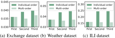
Impact of Multi-order Stacked Architecture As aforementioned in Section 4.2, we organize DERITS as a parallelstacked architecture for multi-order fusion. Thus we aim to study the impact of such a stacked architecture. In contrast to multi-order stacked DERITS, we have considered another situation of individual-order DERITS that removes the parallel-stacked architecture. Figure 3 has shown the performance comparison with individual-order DERITS in the Exchange, ILI, and Weather datasets. It can be easily observed that without the parallel-stacked architecture for multi-order fusion, the individual-order DERITS achieves much worse performance than the original one even under different orders, which signifies the necessity of our multi-order design in the frequency derivative learning architecture.
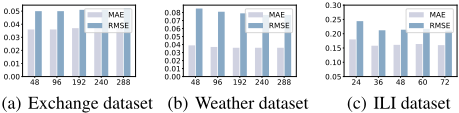
Lookback Analysis We aim to examine the impact of the lookback window on forecasting performance of DERITS. Figure 4 has demonstrated the experimental results on the Exchange, Weather, and ILI datasets. Specifically, we maintain the prediction length as 96 and and vary the lookback length from 48 to 288 on Exchange and Weather datasets. For the ILI dataset, we keep the prediction length at 36 and alter the lookback window size from 24 to 72. From the results, we can observe that in most cases, larger lookback length would bring up less prediction errors; this is because larger input includes more temporal information. Also, larger input length would also bring more noises hindering forecasting, while our DERITS can achieve comparatively stable performance.
| Length | 96 | 192 | 336 | 480 |
|---|---|---|---|---|
| NS-FEDformer | 137.7 | 160.4 | 192.8 | 227.2 |
| NS-Autoformer | 44.41 | 59.23 | 78.29 | 101.5 |
| NS-Transformer | 30.24 | 41.38 | 50.21 | 61.88 |
| DERITS | 12.57 | 13.87 | 14.93 | 15.93 |
Efficiency Analysis To conduct the efficiency analysis for our framework, we report the training time of DERITS across various prediction lengths, and we also include the training time of the Non-Stationary transformer [Liu et al., 2022b] for comparison, coupled with its corresponding backbones such as FEDformer, Autoformer and Transformer. The experiments are conducted under the prediction length with the same input length of 96 on the Exchange dataset. As shown in Table 4, the results prominently highlight that our model exhibits superior efficiency metrics. Our DERITS significantly reduces the number of parameters thus enhancing the computation speed. In particular, our model showcases an average speed that is several times faster than the baselines. These findings underscore the efficiency gains achieved by our model, positioning it as a compelling choice for nonstationary time series forecasting.
5.5 Visualization Analysis
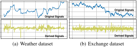
FDT and Non-stationarity To study the Fourier derivative transformation in DERITS, we visualize the original signals and derived signals for comparison. Since the direct outputs of FDT are complex values that are difficult to visualize completely, we thus transform the derived frequency components back to the time domain via inverse FDT, which allows us to show the corresponding time values for visualization. Specifically, we choose two non-stationary time series from the Weather dataset and Exchange dataset, respectively. As shown in Figure 5, we can observe the original signals have included obvious non-stationary oscillations and trends. In contrast, the derived signals exhibit a larger degree of stationarity compared with raw data. This further reveals that learning in the derivative representation of signals is more stationary and thus can achieve better performance.
Case Study of Forecasting To further analysis the model performance, we carry out the case study for non-stationary time series forecasting. Figure 6 demonstrates the visualization of forecasting results of DERITS and NSTransformer [Liu et al., 2022b] with the prediction length as 96 and lookback length as 96. Upon careful observation of it, it becomes evident that DERITS can be capable of aligning with the ground truth when the time series distribution is largely shifted, while the baseline method deviates from the true values. This demonstrates our model's adaptability to shifts. We include more visualizations in Appendix E.
6 Conclusion Remarks
In this paper, we propose to address non-stationary time series forecasting from the frequency perspective. Specifically, we utilize the whole frequency spectrum for the transformation of time series in order to make full use of time series distribution. Motivated by this point, we propose a deep frequency derivative learning framework DERITS for non-stationary forecasting, which is mainly composed of the Frequency Derivative Transformation and the Order-adaptive Fourier Convolution Network with a parallel-stacked architecture. Extensive experiments on real-world datasets have demonstrated its superiority. Moreover, distribution shifts and non-stationarity are actually a pervasive and crucial topic for time series forecasting. Thus we hope that the new perspective of frequency derivation together with the DERITS framework can facilitate more future related research.
Acknowledgments
This work was partially supported by the National Natural Science Foundation of China (No. 62072153) the Anhui Provincial Key Technologies R&D Program (No. 2022h11020015), the Shanghai Baiyulan Talent Plan Pujiang Project (23PJ1413800), and the National Natural Science Foundation of China (No. 623B2043).
@inproceedings{ijcai2024p436,
  title     = {Deep Frequency Derivative Learning for Non-stationary Time Series Forecasting},
  author    = {Fan, Wei and Yi, Kun and Ye, Hangting and Ning, Zhiyuan and Zhang, Qi and An, Ning},
  booktitle = {Proceedings of the Thirty-Third International Joint Conference on
               Artificial Intelligence, {IJCAI-24}},
  publisher = {International Joint Conferences on Artificial Intelligence Organization},
  editor    = {Kate Larson},
  pages     = {3944--3952},
  year      = {2024},
  month     = {8},
  note      = {Main Track},
  doi       = {10.24963/ijcai.2024/436},
  url       = {https://doi.org/10.24963/ijcai.2024/436},
}
TY - CPAPER TI - Deep Frequency Derivative Learning for Non-stationary Time Series Forecasting AU - Fan, Wei AU - Yi, Kun AU - Ye, Hangting AU - Ning, Zhiyuan AU - Zhang, Qi AU - An, Ning T2 - Proceedings of the Thirty-Third International Joint Conference on Artificial Intelligence, IJCAI-24 PB - International Joint Conferences on Artificial Intelligence Organization PY - 2024 SP - 3944 EP - 3952 DO - 10.24963/ijcai.2024/436 UR - https://doi.org/10.24963/ijcai.2024/436 ER -Copied
Machine-readable versions of this paper, for tools and AI agents:





