
Symplectic Neural Gaussian Processes for Meta-learning Hamiltonian Dynamics
Proceedings of the Thirty-Third International Joint Conference on Artificial Intelligence. Main Track. Pages 4210-4218.
https://doi.org/10.24963/ijcai.2024/465
Keywords
- Machine Learning: ML: Meta-learning
- Multidisciplinary Topics and Applications: MTA: Physical sciences
Abstract
We propose a meta-learning method for modeling Hamiltonian dynamics from a limited number of data. Although Hamiltonian neural networks have been successfully used for modeling dynamics that obey the energy conservation law, they require many data to achieve high performance. The proposed method meta-learns our neural network-based model using datasets in various dynamical systems, such that our model can predict vector fields of unseen systems. In our model, a system representation is inferred from given small data using an encoder network. Then, the system-specific vector field is predicted by modeling the Hamiltonian using a Gaussian process (GP) with neural network-based mean and kernel functions that depend on the inferred system representation. This GP-based Hamiltonian allows us to analytically obtain predictions that are adapted to small data while imposing the constraint of the conservation law. The neural networks are shared across systems, which enables us to learn knowledge from multiple systems, and use it for unseen systems. In our experiments, we demonstrate that the proposed method outperforms existing methods for predicting dynamics from a small number of observations in target systems.
- [Baxter, 2000] Jonathan Baxter. A model of inductive bias learning. Journal of Artificial Intelligence Research, 12:149-198, 2000.
- [Bertinetto et al., 2018] Luca Bertinetto, Joao F Henriques, Philip Torr, and Andrea Vedaldi. Meta-learning with dif- ferentiable closed-form solvers. In International Confer- ence on Learning Representations, 2018.
- [Braun and Kivshar, 1998] Oleg M Braun and Yuri S Kivshar. Nonlinear dynamics of the Frenkel-Kontorova model. Physics Reports, 306(1-2):1-108, 1998.
- [Chang and Zeng, 2023] Cheng Chang and Tieyong Zeng. A hybrid data-driven-physics-constrained Gaussian pro- cess regression framework with deep kernel for uncer- tainty quantification. Journal of Computational Physics, 486:112129, 2023.
- [Chang et al., 2023] Cheng Chang, Tieyong Zeng, and Zhouping Xin. A conservative hybrid physics-informed neural network method for ampère-Nernst-Planck equa- tions. SSRN 4435273, 2023.
- [Che et al., 2018] Zhengping Che, Sanjay Purushotham, Kyunghyun Cho, David Sontag, and Yan Liu. Recurrent neural networks for multivariate time series with missing values. Scientific Reports, 8(1):6085, 2018.
- [Chen et al., 2018] Ricky TQ Chen, Yulia Rubanova, Jesse Bettencourt, and David K Duvenaud. Neural ordinary dif- ferential equations. Advances in Neural Information Pro- cessing Systems, 31, 2018.
- [Chen et al., 2020] Zhengdao Chen, Jianyu Zhang, Martin Arjovsky, and Léon Bottou. Symplectic recurrent neural networks. In International Conference on Learning Rep- resentations, 2020.
- [Chen et al., 2021] Yuhan Chen, Takashi Matsubara, and Takaharu Yaguchi. Neural symplectic form: learn- ing Hamiltonian equations on general coordinate sys- tems. Advances in Neural Information Processing Sys- tems, 34:16659-16670, 2021.
- [Chen et al., 2022a] Yuyan Chen, Bin Dong, and Jinchao Xu. Meta-MgNet: Meta multigrid networks for solving parameterized partial differential equations. Journal of computational physics, 455:110996, 2022.
- [Chen et al., 2022b] Zhijie Chen, Mingquan Feng, Junchi Yan, and Hongyuan Zha. Learning neural Hamiltonian dynamics: a methodological overview. arXiv preprint arXiv:2203.00128, 2022.
- [Daniels and Nemenman, 2015] Bryan C Daniels and Ilya Nemenman. Efficient inference of parsimonious phe- nomenological models of cellular dynamics using S- systems and alternating regression. PLOS ONE, 10(3):e0119821, 2015.
- [Dormand and Prince, 1980] John R Dormand and Peter J Prince. A family of embedded runge-kutta formulae. Jour- nal of Computational and Applied Mathematics, 6(1):19- 26, 1980.
- [Finn et al., 2017] Chelsea Finn, Pieter Abbeel, and Sergey Levine. Model-agnostic meta-learning for fast adapta- tion of deep networks. In Proceedings of the 34th Inter- national Conference on Machine Learning, pages 1126- 1135, 2017.
- [Finzi et al., 2020] Marc Finzi, Ke Alexander Wang, and Andrew G Wilson. Simplifying Hamiltonian and Lagrangian neural networks via explicit constraints. Advances in Neural Information Processing Systems, 33:13880-13889, 2020.
- [Fortuin et al., 2019] Vincent Fortuin, Heiko Strathmann, and Gunnar Rätsch. Meta-learning mean functions for Gaussian processes. arXiv preprint arXiv:1901.08098, 2019.
- [Garnelo et al., 2018] Marta Garnelo, Dan Rosenbaum, Christopher Maddison, Tiago Ramalho, David Saxton, Murray Shanahan, Yee Whye Teh, Danilo Rezende, and SM Ali Eslami. Conditional neural processes. In Inter- national Conference on Machine Learning, pages 1690- 1699, 2018.
- [Graves and Graves, 2012] Alex Graves and Alex Graves. Long short-term memory. Supervised sequence labelling with recurrent neural networks, pages 37-45, 2012.
- [Greydanus et al., 2019] Samuel Greydanus, Misko Dzamba, and Jason Yosinski. Hamiltonian neural networks. Advances in Neural Information Processing Systems, 32, 2019.
- [Haussler, 1988] David Haussler. Quantifying inductive bias: AI learning algorithms and valiant's learning frame- work. Artificial Intelligence, 36(2):177-221, 1988.
- [He and Zou, 2021] Horace He and Richard Zou. functorch: JAX-like composable function transforms for PyTorch. https://github.com/pytorch/functorch, 2021. Link
- [Iwata and Tanaka, 2022] Tomoharu Iwata and Yusuke Tanaka. Few-shot learning for spatial regression via neural embedding-based Gaussian processes. Machine Learning, pages 1-19, 2022.
- [Kingma and Ba, 2015] Diederik P. Kingma and Jimmy Ba. Adam: A method for stochastic optimization. In Interna- tional Conference on Learning Representations, 2015.
- [Lee et al., 2021] Seungjun Lee, Haesang Yang, and Woojae Seong. Identifying physical law of Hamiltonian systems via meta-learning. In International Conference on Learn- ing Representations, 2021.
- [Leonessa et al., 2001] Alexander Leonessa, Wassim M Haddad, and VijaySekhar Chellaboina. Nonlinear sys- tem stabilization via hierarchical switching control. IEEE Transactions on Automatic Control, 46(1):17-28, 2001.
- [Mattheakis et al., 2022] Marios Mattheakis, David Sondak, Akshunna S Dogra, and Pavlos Protopapas. Hamiltonian neural networks for solving equations of motion. Physical Review E, 105(6):065305, 2022.
- [Paszke et al., 2019] Adam Paszke, Sam Gross, Francisco Massa, Adam Lerer, James Bradbury, Gregory Chanan, Trevor Killeen, Zeming Lin, Natalia Gimelshein, Luca Antiga, et al. Pytorch: An imperative style, high- performance deep learning library. Advances in Neural Information Processing Systems, 32, 2019.
- [Patacchiola et al., 2020] Massimiliano Patacchiola, Jack Turner, Elliot J Crowley, Michael O'Boyle, and Amos J Storkey. Bayesian meta-learning for the few-shot setting via deep kernels. Advances in Neural Information Pro- cessing Systems, 33:16108-16118, 2020.
- [Psaros et al., 2022] Apostolos F Psaros, Kenji Kawaguchi, and George Em Karniadakis. Meta-learning PINN loss functions. Journal of Computational Physics, 458:111121, 2022.
- [Raghu et al., 2020] Aniruddh Raghu, Maithra Raghu, Samy Bengio, and Oriol Vinyals. Rapid learning or fea- ture reuse? Towards understanding the effectiveness of MAML. In International Conference on Learning Rep- resentations, 2020.
- [Rath et al., 2021] Katharina Rath, Christopher G Albert, Bernd Bischl, and Udo von Toussaint. Symplectic Gaus- sian process regression of maps in Hamiltonian systems. Chaos: An Interdisciplinary Journal of Nonlinear Science, 31(5):053121, 2021.
- [Ravi and Larochelle, 2017] Sachin Ravi and Hugo Larochelle. Optimization as a model for few-shot learning. In International Conference on Learning Representations, 2017.
- [Rothfuss et al., 2021] Jonas Rothfuss, Vincent Fortuin, Martin Josifoski, and Andreas Krause. PACOH: Bayes- optimal meta-learning with PAC-guarantees. In Inter- national Conference on Machine Learning, pages 9116- 9126, 2021.
- [Snell et al., 2017] Jake Snell, Kevin Swersky, and Richard Zemel. Prototypical networks for few-shot learning. Ad- vances in Neural Information Processing Systems, 30, 2017.
- [Tanaka et al., 2022] Yusuke Tanaka, Tomoharu Iwata, and Naonori Ueda. Symplectic spectrum Gaussian processes: Learning Hamiltonians from noisy and sparse data. In Ad- vances in Neural Information Processing Systems, 2022.
- [Thangamuthu et al., 2022] Abishek Thangamuthu, Gunjan Kumar, Suresh Bishnoi, Ravinder Bhattoo, NM Krish- nan, and Sayan Ranu. Unravelling the performance of physics-informed graph neural networks for dynamical systems. Advances in Neural Information Processing Sys- tems, 35:3691-3702, 2022.
- [Tong et al., 2021] Yunjin Tong, Shiying Xiong, Xingzhe He, Guanghan Pan, and Bo Zhu. Symplectic neural net- works in Taylor series form for Hamiltonian systems. Journal of Computational Physics, 437:110325, 2021.
- [Toth et al., 2020] Peter Toth, Danilo J Rezende, Andrew Jaegle, Sébastien Racanière, Aleksandar Botev, and Irina Higgins. Hamiltonian generative networks. In Interna- tional Conference on Learning Representations, 2020.
- [Vinyals et al., 2016] Oriol Vinyals, Charles Blundell, Tim- othy Lillicrap, Daan Wierstra, et al. Matching networks for one shot learning. In Advances in Neural Information Processing Systems, pages 3630-3638, 2016.
- [Vovk, 2013] Vladimir Vovk. Kernel ridge regression. Em- pirical Inference: Festschrift in Honor of Vladimir N. Vap- nik, pages 105-116, 2013.
- [Wilson et al., 2016] Andrew Gordon Wilson, Zhiting Hu, Ruslan Salakhutdinov, and Eric P Xing. Deep kernel learn- ing. In Artificial intelligence and statistics, pages 370- 378, 2016.
- [Zhong et al., 2020] Yaofeng Desmond Zhong, Biswadip Dey, and Amit Chakraborty. Symplectic ODE-net: Learn- ing Hamiltonian dynamics with control. In International Conference on Learning Representations, 2020.
References were extracted automatically from the PDF and may contain errors.
Full text extracted automatically from the PDF; figures, tables and equations may differ. The PDF is the version of record.
1 Introduction
Modeling the dynamics of physical systems given time-series data is important in various fields, such as physics [Braun and Kivshar, 1998], biology [Daniels and Nemenman, 2015], and engineering [Leonessa et al., 2001]. Neural networks have been widely used for modeling the dynamics due to its high representation learning capability [Chen et al., 2018; Che et al., 2018]. By incorporating inductive biases, we can learn underlying behaviors beyond the given data [Haussler, 1988; Baxter, 2000; Chang and Zeng, 2023; Chang et al., 2023]. Hamiltonian neural networks (HNNs) [Greydanus et al., 2019; Mattheakis et al., 2022; Chen et al., 2022b] incorporate an inductive bias of physics, where the total energy of the system is conserved. HNNs have been shown to be effective in learning Hamiltonian dynamics from data [Finzi et al., 2020;
Zhong et al., 2020; Chen et al., 2020; Chen et al., 2021; Tong et al., 2021; Tanaka et al., 2022]. However, they require a large amount of data for training. In real-world applications, preparing sufficient data incurs a high cost and is time-consuming.
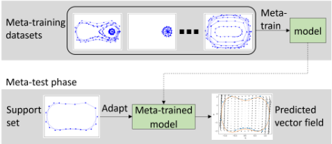
In this paper, we propose a meta-learning method for modeling Hamiltonian dynamics from a limited number of data. The proposed method meta-learns our neural network-based model using meta-training datasets in various dynamical systems, such that it can model unseen systems given small data. Figure 1 illustrates our problem setting.
The meta-learning framework is formulated as a bilevel optimization, where the inner optimization corresponds to the adaptation of the system-specific components in our model, and the outer optimization corresponds to the estimation of the system-shared components. We model a system-specific Hamiltonian using a Gaussian process (GP), by which we can incorporate the inductive bias of the energy conservation law. By this GP framework, we can analytically obtain a vector field that is adapted to given small data in the inner optimization. This enables effective backpropagation through the inner optimization, which is required for each outer optimization iteration.
In system-specific GPs for Hamiltonian, we use neural network-based mean and kernel functions that depend on a system representation. The system representation is obtained using an encoder network from given small data. Using the system representation yields a system-specific vector field. With the neural networks, we can flexibly model various vector fields. The neural networks are shared across all systems, by which we can learn common knowledge in multiple systems, and use the knowledge for newly given systems. We call our model the symplectic neural Gaussian process (SNGP) since our neural network-based GP incorporates the symplectic structure for the energy conservation law. The neural network parameters are trained by minimizing the expected test error of vector fields when a few data are given, which is calculated using meta-training datasets by an episodic training framework [Finn et al., 2017].
The main contributions of this paper are as follows: 1) We propose a neural network-based GP model for modeling Hamiltonian dynamics that obeys the conservation law, where the adaptation to given data can be performed in a closed form. 2) We develop a meta-learning procedure for our model to improve the expected test predictive performance on vector fields. 3) We empirically demonstrate that the proposed method performs well in modeling Hamiltonian dynamics with a limited number of data.
2 RelatedWork
Meta-learning has been successfully used for improving the prediction performance on unseen tasks with few data by learning to learn from various tasks [Finn et al., 2017; Vinyals et al., 2016; Snell et al., 2017; Rothfuss et al., 2021; Psaros et al., 2022; Chen et al., 2022a]. However, these existing methods are not for Hamiltonian dynamics except for [Lee et al., 2021]. [Lee et al., 2021] proposed to metalearn HNNs using gradient-based methods [Finn et al., 2017; Raghu et al., 2020], which require iterative optimization procedures for adaptation. The backpropagation through such procedures is costly in terms of memory, and the total number of iterations must be kept small [Finn et al., 2017]. On the other hand, the proposed method can perform adaptation in a closed form with GPs. The effectiveness of closed-form adaptation has been shown in meta-learning for classification and regression tasks [Bertinetto et al., 2018; Fortuin et al., 2019; Patacchiola et al., 2020; Iwata and Tanaka, 2022]. Although GPs have been used for modeling Hamiltonian [Rath et al., 2021; Tanaka et al., 2022], these methods cannot perform meta-learning. The proposed method enables meta-learning by effectively integrating the GP-based Hamiltonian in neural networks. Our model is related to neural processes (NPs) [Garnelo et al., 2018] as both use neural networks for task (system) representation inference and for prediction with inferred task representations. However, since NP prediction is based on fully parametric models, they are less flexible in adapting to given data than GPs. In contrast, our GP-based model enables swift adaptation by explicitly solving an optimization problem for adaptation.
3 Preliminaries: HamiltonianMechanics
In the Hamiltonian system, the continuous-time evolution is described in phase space, which is the product space of generalized coordinates xq = (xq1 , . . . , xqM ) and generalized momenta xp = (xp1 , . . . , xpM ), where M is the degree of freedom. Let x = (xq , xp ) ∈ RJ , be a state of the system, where J = 2M. The system's evolution is determined by Hamiltonian H(x) : RJ → R, which denotes the system's total energy. In particular, the dynamics of a Hamiltonian system with additive dissipative terms is given by
where ∇H(x) is the gradient of the Hamiltonian with respect to state x, A ∈ RJ×J is a skew-symmetric matrix, R ∈ RJ×J is a positive semi-definite dissipation matrix, I is the identity matrix, and O is the zero matrix. The dynamics of this system conserves the total energy when R = O. An example of the dissipation matrix is R = diag(0, . . . , 0, r1, . . . , rM), representing a dissipative system with friction coefficient rm ≥ 0. Eq. (1) defines the time derivatives of the state by function f(x) : RJ → RJ , which is a special kind of vector field that has a symplectic geometric structure (called Hamiltonian vector field or symplectic gradient).
The Hamiltonian neural network (HNN) is a representative method for modeling the dynamics that obeys Hamiltonian mechanics without manually designed Hamiltonians. In HNNs, a Hamiltonian is modeled by a neural network, and the dynamics is derived using Eq. (1) as follows,
where NN is a neural network. The gradient of the neural network is calculated with automatic differentiation [Paszke et al., 2019]. The parameters of the HNN are estimated by minimizing the error between observed and predicted vector fields, ‖ f - ˆ fHNN(x) ‖2 .
4 ProposedMethod
4.1 ProblemFormulation
In the meta-training phase, we are given time-series datasets of D dynamical systems, {Dd}Dd=1 , where Dd = {{(xdbn, fdbn)}Ndb n=1 }Bd b=1 is Bd sequences in the dth system, xdbn ∈ RJ is the nth state of the rth sequence, fdbn ∈ RJ is its time derivative, and Nrd is the number of observations. In the meta-test phase, we are given a small number of timeseries data S = {{(xSbn , f S bn )}N S n=1 }BS b=1 , which are called a support set, in an unseen system, which is different from the meta-training systems. Our aim is to predict the vector fields, which are the time derivatives of the system's states, and to forecast the time-series in such meta-test systems, as shown in Figure 1. We assume that all systems obey Hamiltonian dynamics with additive dissipation, although the Hamiltonians are unknown, and the Hamiltonians are different across systems. When analytic time derivatives are unavailable, we obtain them by calculating their finite difference approximation from the sequences of the states.
4.2 Symplectic Neural Gaussian Process Model
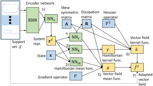
Our symplectic neural Gaussian process (SNGP) model gives system-specific vector field ˆ f S (x) that obey Hamiltonian dynamics given support set S. We use superscript S when the function or variable depends on support set S. Figure 2 illustrates our model.
First, we obtain system representation zS ∈ RKz from support set S using the following encoder network,
where RNN is a recurrent neural network (RNN), NNz is a feed-forward neural network, and [·, ·] represents the vector concatenation. With the RNN, we can extract information on the dynamics in each sequence with arbitrary lengths. The encoder network is a permutation invariant neural network [Che et al., 2018], which can handle an arbitrary number of sequences, and which can obtain a system representation that does not depend on the order of sequences. Here, we assume the time-series are regularly sampled. In the case of irregularly-sampled time series, we can additionally input the timestamp to the RNN as in [Che et al., 2018], [xSbn , f S bn , tSbn ], instead of [xSbn , f S bn ], where tSbn is the nth timestamp of the rth sequence.
Next, we model system-specific Hamiltonian HS by the following GP with deep kernels [Wilson et al., 2016],
where NNm : RJ+Kz → R is a mean function based on a feed-forward neural network, γ is a deep kernel function based on the RBF kernel,
α, β, η ∈ R+ are the kernel parameters, NNk : RJ+Kz → RKg is a feed-forward neural network, and δ(x, x′ ) = 1 if x and x′ are identical, and zero otherwise. With system representation zS for the input of neural networks, NNm and NNk, we can make their outputs depend on support set S. With deep kernels, we can flexibly transform states such that the GP can model the Hamiltonian appropriately. When the system is dissipative, elements in the dissipation matrix r = (r1, . . . , rM) is obtained from system representation zS as follows,
where NNr : RKz → RM is a feed-forward neural network. Neural networks, RNN, NNz, NNm, and NNk, are shared across different systems, which enables us to learn knowledge that is useful across systems, and use it for unseen systems.
Since (A-R)∇ is a linear operator, and a GP with linear transformation is again a GP [Rath et al., 2021], systemspecific vector field f S (x) = (A - R)∇HS (x) is represented by the following a multi-output GP using Eqs. (1,4),
where
and ∇2 is the Hessian operator. The gradient and Hessian operators are calculated with automatic differentiation [Paszke et al., 2019; He and Zou, 2021]. By using the GP with deep kernels, we can model a system-specific vector field that obey Hamiltonian dynamics.
Since the prior distribution of the vector field is a GP in Eq. (7), the predictive value of the vector field adapted to support set S, which is the posterior mean of the GP, is given by
where K ∈ RBSN S J×BSN S J is the kernel matrix evaluated between states in the support set, KbN S+n,b′N S+n′ = k(xSbn , xSb′ n′ , zS ), k = ((k(x, xbn, zS ))N S n=1 )BS b=1 ∈ RBSN S J×J is the kernels evaluated between state x and states in the support set, f S = ((f S bn ))N S n=1 )BS b=1 ∈ RBSN S J
is the observed vector fields of the support set, and m = (µ(xSbn ))N S n=1 )BS b=1 ∈ RBSN S J is the predicted vector fields of the support set by mean function µ.
Eq. (10) minimizes the mean squared error on the support set with a regularizer [Vovk, 2013]. An advantage of our model is that the predictive value given the support set is analytically calculated without iterative optimization, by which we can minimize the expected test error effectively based on a stochastic gradient descent method in our metalearning framework.
4.3 Meta-learning
The system-shared parameters θ in the SNGP are parameters in neural networks, RNN, NNz, NNm, NNk, NNr, and kernel parameters, α, β, η. We train them by minimizing the expected test mean squared error using an episodic training framework [Ravi and Larochelle, 2017],
where Ed represents the expectation over systems, and ES,Q∼Dd represents the expectation over support and query sets that are generated from meta-training dataset Dd in the dth system. Query set Q = {{(xQbn , f Q bn )}N Q n=1 }BQ b=1 is a timeseries data set that is different from the support set used for adapting GP, by which we can evaluate the test error. Minimizing our meta-learning loss in Eq. (11) is a bilevel optimization problem. In the inner optimization, a systemspecific prediction model is adapted to the support set based on the GP framework as described in Section 4.2. In the outer optimization, system-shared parameters are estimated by minimizing the error on the query set when the systemspecific prediction model obtained in the inner optimization is used.
Algorithm 1 shows the meta-training procedure of the proposed model. The expectation in Eq. (11) is approximated by the Monte Carlo method in Lines 3-5, where a system, support and query instances are randomly sampled from the meta-training datasets. In Line 7, the inner optimization is performed, which corresponds to obtaining the posterior mean of the GP in Eq. (10). When the distributions of systems are the same between meta-training and meta-test phases, and a sufficient number of meta-training datasets are given, the expected error in the meta-test phase is improved by the minimization in Eq. (11).
The computational complexity of calculating the test error for a query set is O((BSN SJ)3 ) since we need the inverse of the kernel matrix whose size is BSN SJ × BSN SJ. In few-shot settings, which is our focus, the number of support instances BSN S is small, and the proposed method can metalearn our model efficiently.
5 Expriments
5.1 Data
We used six types of dynamical systems: mass-spring, pendulum, and Duffing systems without friction, and those with Algorithm 1 Meta-learning procedure of our SNGP model.
Input: Meta-training data D, number of support sequences BS , number of support observations N S , number of query sequences BQ, number of query observations N Q
Output: Trained model parameters θ
- 1: Initialize model parameters θ.
- 2: while End condition is satisfied do
- 3: Randomly select system index d from {1, · · · ,D}.
- 4: Randomly sample BS sequences with N S observations for support set S fromDd.
- 5: Randomly sample BQ sequences with N Q observations for query set Q from Dd such that there is no overlap between the support and query sequences.
- 6: Calculate system representation zS using Eq. (3).
- 7: Calculate predictive vector field values ˆ f S (x) adapted to support set S using Eq. (10).
- 8: Calculate test error 1 N Q ∑(x,f)∈Q ‖ f - ˆ f S (x) ‖2 .
- 9: Update system-shared parameters θ using the gradient of the test error by a stochastic gradient method.
- 10: end while
friction. In each type, physical parameters were different across systems as in [Lee et al., 2021].
The Hamiltonian of the one-dimensional mass-spring system without friction is given by H(x) = 12 kxq2 + xp2 2m , where k is the spring constant, and m is the mass constant. For each system, k ∈ [5, 6] and m ∈ [0.5, 1.5] were determined uniformly randomly within their given range. The initial coordinates for each sequence were determined uniformly randomly from [1, 2].
The Hamiltonian of the pendulum system without friction with a single degree of freedom is H(x) = mgℓ(1 - cos(xq )) + xp2 2mℓ2 , where g is the gravitational constant, m is the mass constant, and ℓ is the length of the pendulum. Length ℓ ∈ [0.5, 1.5] was determined uniformly randomly for each system. and g = 9.8 and m = 1 were fixed for all systems. The initial coordinates were determined uniformly randomly from [1, π].
The Hamiltonian of the Duffing system without friction is H(x) = 1 2 xp2 + α4 xq4 + β2 xq2 , where β = [-10, 0] was determined uniformly randomly for each system, and α = 10 was fixed. The initial coordinates were randomly determined from [0.5, 1.5]. In systems with friction, the friction coefficient was uniformly randomly determined in [0, 1].
In all systems, a state is a two-dimensional vector, x = (xq , xp ) ∈ R2 , or M = 2. and the initial momentum was set to zero. For each system, 30 sequences of the states were sampled at a frequency of five Hz for four seconds with additive Gaussian noise with standard deviation 10-2 . For each type, five systems were used for meta-training, three for metavalidation, and six for meta-test. The number of support sequences was {1, 3, 5}, and the number of query sequences was 10. The time derivatives were obtained by the central finite difference approximation. The experiments were conducted ten times by resampling the meta-training, metavalidation, and meta-test systems.
For the evaluation measurement, we used the test mean squared errors of the predicted trajectories of the query sets in the meta-test systems given the initial states. To obtain trajectories, we integrated models with the fourth-order RungeKutta integrator in scipy.integrate.solve ivp with error tolerance to 10-12 [Dormand and Prince, 1980].
5.2 ComparedMethods
We compared the proposed method (Ours) with the following methods: Hamiltonian neural process (HNP), meta-learning Hamiltonian neural network (MHNN) [Lee et al., 2021], meta-learning Gaussian process (MGP) [Iwata and Tanaka, 2022], neural process (NP) [Garnelo et al., 2018], metalearning neural network (MNN), Symplectic Gaussian process (SGP) [Rath et al., 2021], Hamiltonian neural network (HNN) [Greydanus et al., 2019], neural network (NN), and Gaussian process (GP). Ours, HNP, HHNN, MGP, NP, and MNN are meta-learning methods that give system-adapted models by training with multiple meta-training systems. Ours, HNP, MHNN, HGP, and HNN use the inductive bias of the conservation law with Hamiltonian.
With neural process-based methods (HNP and NP), system representations were obtained by Eq. (3) as the same with the proposed method. HNP used a neural network for modeling Hamiltonian H(x), and NP used it for modeling vector field f (x), where the system representation and the state were taken as the input. HNP corresponds to the proposed method without adaptation with GPs. MHNN and MNN used modelagnostic meta-learning (MAML) [Finn et al., 2017] for metalearning, where MHNN used a Hamiltonian neural network, and MNN used a feed-forward neural network for their models. MGP used a GP with deep kernel for modeling the vector field, where the GP was adapted for each system, and the deep kernel was shared across systems. SGP used a GP with the Gaussian kernel for modeling the Hamiltonian. In HNN and NN, a neural network was shared across all systems, and trained using the meta-training datasets. In GP, a GP with the Gaussian kernel was adapted for each system.
5.3 Settings
For obtaining system representation in Eq. (3), we used the bidirectional LSTM [Graves and Graves, 2012] for RNN with 32 hidden units, where the sequence of the states was used for input. For NNz and NNk, we used three-layered feedforward neural networks with 32 hidden and output units. For NNm, we used four-layered feed-forward neural networks with 32 hidden units. For the activation function, we used the hyperbolic tangent. We optimized our models using Adam [Kingma and Ba, 2015] with learning rate 10-3 , and batch dataset size four. The meta-validation datasets were used for early stopping, for which the maximum number of meta-training epochs was 5,000.
In the compared methods, we used the same neural network architectures and training procedures as the proposed method. In MAML-based methods (MHNN and MNN), we used learning rate 10-2 and five epochs for inner optimization. For neural networks in HNP, MHNN, NP, HNN, and NN, we used four-layered feed-forward neural networks. In MGP, HGP, and GP, kernel parameters of RBF kernels were optimized using the meta-training datasets.
We implemented all methods with PyTorch [Paszke et al., 2019]. For gradient and Hessian operators in Eqs. (8,9), we used functorch [He and Zou, 2021].
5.4 Results
Table 1 shows the test mean squared errors of trajectories. In all cases, the proposed method achieved the lowest error. The test error by HNP was high since the system adaptation is modeled only by neural networks. On the other hand, the proposed method performs the system adaptation by minimizing the training error, which leads to better performance. Since MHNN uses an iterative optimization with a small number of steps for system adaptation, it was difficult to adapt to various systems. In contrast, the proposed method can obtain a solution of the inner optimization in a closed form using GPs. MGP, NP, MNN, NN and GP do not use the inductive bias on the Hamiltonian systems. Therefore, the performance of these methods was low. Since HNN and NN use the same models for all systems, they cannot handle the difference among systems, and resulted in their high error. Since GP modeled the vector field for each system, its performance was low, especially when the number of support sequences was small. The proposed method achieved better performance with a small number of support sequences using knowledge in other systems with different Hamiltonians by sharing neural networks.
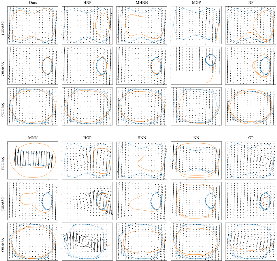
Figure 3 shows the predicted trajectories on the Duffing without friction system with one support sequence per system. The proposed method successfully estimated systemspecific vector fields and trajectories. The methods that model the Hamiltonian, i.e., the proposed method, HNP, MNN, HGP, and HNN, estimated the vector field that obeyed the conservation law. On the other hand, the other methods estimated diverging or decaying vector fields, even though it was a conservation system. These results indicate the effectiveness of modeling the Hamiltonian.
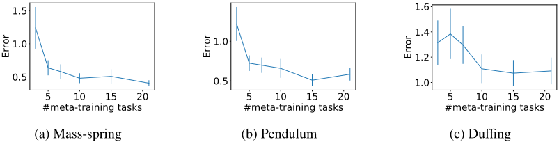
Figure 4 shows the test mean squared errors with different numbers of meta-training systems. As the number of the meta-training systems increased, the error decreased. This result indicates that the proposed method improved the performance by using knowledge in different systems.
Table 2 shows the test mean squared errors in ablation study. Removing system representations, neural networkbased mean functions, and neural network-based kernel functions decreased the performance. This result indicates that the system-shared neural networks in our model is important for meta-learning to share knowledge across different dynamical systems. Note that all methods in Table 2 are newly proposed in this paper, and our model can adapt to each system based on the GP framework even without system representations.
Additional experimental results, such as the errors of predicted vector fields, the errors of predicted total energies, computational time for meta-training, and computational time for predicting vector fields, are shown in the supplementary material. In most of the cases, the proposed method outperformed the compared methods for predicting vector fields. The proposed method achieved low errors in all cases for predicting total energies. In the other methods, predicted total energies were sometimes diverged from the ground truth, which resulted in high variance of their errors. The proposed method took a longer time than HNP, MGP, and HGP since it contains them as components. The meta-training time by the proposed method was shorter than MAML-based methods (MHNN and MNN) since the MAML-based methods need iterative optimization for system adaptation. The inference time by the proposed method was short for predicting vector fields given meta-trained models.
| N S | Ours | HNP | MHNN | MGP | NP | MNN | HGP | HNN | NN | GP |
|---|---|---|---|---|---|---|---|---|---|---|
| 1 | 0.638 | 1.543 | 2.783 | 3.962 | 1.502 | 1.067 | 1.687 | 5.209 | 3.390 | 2.892 |
| 3 | 0.669 | 1.809 | 3.969 | 1.856 | 1.688 | 1.145 | 1.250 | 5.209 | 3.390 | 1.367 |
| 5 | 0.649 | 1.497 | 3.265 | 1.500 | 1.696 | 1.304 | 0.879 | 5.209 | 3.390 | 1.083 |
| (b) Mass-spring with friction | ||||||||||
| N S | Ours | HNP | MHNN | MGP | NP | MNN | HGP | HNN | NN | GP |
| 1 | 0.217 | 5.994 | 0.757 | 1.834 | 0.454 | 0.493 | 0.834 | 1.043 | 1.068 | 1.341 |
| 3 | 0.183 | 6.302 | 0.738 | 0.606 | 0.504 | 0.446 | 0.511 | 1.043 | 1.068 | 0.527 |
| 5 | 0.192 | 6.269 | 0.721 | 0.418 | 0.587 | 0.454 | 0.451 | 1.043 | 1.068 | 0.370 |
| (c) Pendulumwithout friction | ||||||||||
| N S | Ours | HNP | MHNN | MGP | NP | MNN | HGP | HNN | NN | GP |
| 1 | 0.723 | 1.542 | 9.312 | 4.317 | 2.055 | 3.844 | 8.556 | 7.468 | 4.469 | 7.339 |
| 3 | 0.708 | 1.715 | 10.864 | 0.997 | 2.190 | 3.778 | 1.522 | 7.468 | 4.469 | 2.899 |
| 5 | 0.499 | 1.772 | 9.805 | 0.817 | 2.167 | 3.931 | 0.569 | 7.468 | 4.469 | 1.565 |
| (d) Pendulum with friction | ||||||||||
| N S | Ours | HNP | MHNN | MGP | NP | MNN | HGP | HNN | NN | GP |
| 1 | 1.053 | 35.484 | 3.007 | 1.708 | 1.832 | 1.323 | 4.664 | 3.738 | 3.034 | 2.753 |
| 3 | 0.660 | 34.132 | 2.642 | 0.634 | 1.717 | 1.141 | 2.127 | 3.738 | 3.034 | 1.190 |
| 5 | 0.561 | 35.520 | 2.500 | 0.540 | 1.513 | 1.095 | 2.050 | 3.738 | 3.034 | 0.769 |
| (e) Duffing without friction | ||||||||||
| N S | Ours | HNP | MHNN | MGP | NP | MNN | HGP | HNN | NN | GP |
| 1 | 1.384 | 1.574 | 2.776 | 6.663 | 1.338 | 2.067 | 2.968 | 2.195 | 2.158 | 2.402 |
| 3 | 1.306 | 1.503 | 2.354 | 5.421 | 1.186 | 1.657 | 1.819 | 2.195 | 2.158 | 2.140 |
| 5 | 1.251 | 1.350 | 2.276 | 6.826 | 1.318 | 1.654 | 1.526 | 2.195 | 2.158 | 2.013 |
| (f) Duffing with friction | ||||||||||
| N S | Ours | HNP | MHNN | MGP | NP | MNN | HGP | HNN | NN | GP |
| 1 | 0.333 | 20.328 | 0.752 | 1.093 | 0.575 | 0.706 | 1.277 | 0.804 | 1.070 | 0.951 |
| 3 | 0.347 | 21.369 | 0.645 | 1.130 | 0.502 | 0.650 | 0.523 | 0.804 | 1.070 | 0.708 |
| 5 | 0.327 | 22.780 | 0.628 | 1.117 | 0.586 | 0.654 | 0.438 | 0.804 | 1.070 | 0.656 |
| Ours | w/o-zS | w/o-NNm | w/o-NNk |
| 0.650 | 0.684 | 0.826 | 0.852 |
Table 2: Ablation studies of our model: test mean squared errors of trajectories averaged over all cases. 'w/o-zS ' is the proposed method without system representations. 'w/o-NNm' is the proposed method without neural network-based mean functions, where zero mean functions are used. 'w/o-NNk' is the proposed method without neural network-based kernel functions, where state x is directly inputted into RBF kernels.
6 Conclusion
We proposed a neural network-based meta-learning method that effectively extracts common knowledge from data in multiple dynamical systems. The proposed method can learn dynamics that exactly conserves the total energy by modeling Hamiltonian, where a system-specific Hamiltonian adapted to given data is obtained in a closed form using GPs. Our experiments demonstrate that the proposed method achieves better performance than the existing methods with a small number of training data.
Although our results are encouraging as a data-efficient method for modeling Hamiltonian systems, there are some limitations to overcome. First, we plan to apply our method to systems with a larger number of states by improving computational efficiency using random Fourier features for GPs [Tanaka et al., 2022]. Second, we will improve data efficiency of the proposed method further by using constrained HNNs [Finzi et al., 2020] and graph neural networks [Thangamuthu et al., 2022]. Third, we would like to extend our method to find state spaces by combining with Hamiltonian generative networks [Toth et al., 2020].
@inproceedings{ijcai2024p465,
  title     = {Symplectic Neural Gaussian Processes for Meta-learning Hamiltonian Dynamics},
  author    = {Iwata, Tomoharu and Tanaka, Yusuke},
  booktitle = {Proceedings of the Thirty-Third International Joint Conference on
               Artificial Intelligence, {IJCAI-24}},
  publisher = {International Joint Conferences on Artificial Intelligence Organization},
  editor    = {Kate Larson},
  pages     = {4210--4218},
  year      = {2024},
  month     = {8},
  note      = {Main Track},
  doi       = {10.24963/ijcai.2024/465},
  url       = {https://doi.org/10.24963/ijcai.2024/465},
}
TY - CPAPER TI - Symplectic Neural Gaussian Processes for Meta-learning Hamiltonian Dynamics AU - Iwata, Tomoharu AU - Tanaka, Yusuke T2 - Proceedings of the Thirty-Third International Joint Conference on Artificial Intelligence, IJCAI-24 PB - International Joint Conferences on Artificial Intelligence Organization PY - 2024 SP - 4210 EP - 4218 DO - 10.24963/ijcai.2024/465 UR - https://doi.org/10.24963/ijcai.2024/465 ER -Copied
Machine-readable versions of this paper, for tools and AI agents:





