
Temporal Domain Generalization via Learning Instance-level Evolving Patterns
Proceedings of the Thirty-Third International Joint Conference on Artificial Intelligence. Main Track. Pages 4255-4263.
https://doi.org/10.24963/ijcai.2024/470
Keywords
- Machine Learning: ML: Regression
- Machine Learning: ML: Multi-task and transfer learning
- Machine Learning: ML: Incremental learning
- Machine Learning: ML: Classification
Abstract
Temporal Domain Generalization (TDG) aims at learning models under temporally evolving data distributions and achieving generalization to unseen future data distributions following the evolving trend. Existing advanced TDG methods learn the evolving patterns through the collective behaviors observed at the population-level of instances, such as time-varying statistics and parameters, tending to overlook the impact of individual-level instance evolving processes on the decision boundary. However, a major obstacle is that datasets at different timestamps may comprise unrelated instances and there is no inherent existence of the instance-level evolving trajectories, which hinders us from learning how the decision boundary changes. To address the above challenges, we propose a Continuous-Time modelling Optimal Transport trajectories (CTOT) framework in this paper. Specifically, we utilize optimal transport to align the data distributions between each pair of adjacent source domains to construct instance evolving trajectories. Subsequently, they are modelled by a continuous-time model and extrapolated to generate future virtual instances, which help the model to adapt its decision boundary to the future domain. Extensive experiments on multiple classification and regression benchmarks demonstrate the effectiveness of the proposed CTOT framework. The code and appendix are both available on https://github.com/JinYujie99/CTOT.
- [Bai et al., 2023] Guangji Bai, Chen Ling, and Liang Zhao. Temporal domain generalization with drift-aware dynamic neural networks. In The Eleventh International Confer- ence on Learning Representations, 2023.
- [Biloš et al., 2023] Marin Biloš, Kashif Rasul, Anderson Schneider, Yuriy Nevmyvaka, and Stephan Günnemann. Modeling temporal data as continuous functions with stochastic process diffusion. In International Conference on Machine Learning, pages 2452-2470. PMLR, 2023.
- [Blanchard et al., 2021] Gilles Blanchard, Aniket Anand Deshmukh, Ürun Dogan, Gyemin Lee, and Clayton Scott. Domain generalization by marginal transfer learning. The Journal of Machine Learning Research, 22(1):46-100, 2021.
- [Bui et al., 2021] Manh-Ha Bui, Toan Tran, Anh Tran, and Dinh Phung. Exploiting domain-specific features to en- hance domain generalization. Advances in Neural Infor- mation Processing Systems, 34:21189-21201, 2021.
- [Cha et al., 2021] Junbum Cha, Sanghyuk Chun, Kyungjae Lee, Han-Cheol Cho, Seunghyun Park, Yunsung Lee, and Sungrae Park. Swad: Domain generalization by seeking flat minima. Advances in Neural Information Processing Systems, 34:22405-22418, 2021.
- [Chen et al., 2018] Ricky TQ Chen, Yulia Rubanova, Jesse Bettencourt, and David K Duvenaud. Neural ordinary dif- ferential equations. Advances in neural information pro- cessing systems, 31, 2018.
- [Chu et al., 2022] Xu Chu, Yujie Jin, Wenwu Zhu, Yasha Wang, Xin Wang, Shanghang Zhang, and Hong Mei. Dna: Domain generalization with diversified neural averaging. In International Conference on Machine Learning, pages 4010-4034. PMLR, 2022.
- [Courty et al., 2014] Nicolas Courty, Rémi Flamary, and De- vis Tuia. Domain adaptation with regularized optimal transport. In Machine Learning and Knowledge Discovery in Databases: European Conference, ECML PKDD 2014, Nancy, France, September 15-19, 2014. Proceedings, Part I 14, pages 274-289. Springer, 2014.
- [Courty et al., 2017] Nicolas Courty, Rémi Flamary, Amaury Habrard, and Alain Rakotomamonjy. Joint distribution optimal transportation for domain adaptation. Advances in neural information processing systems, 30, 2017.
- [Cuturi, 2013] Marco Cuturi. Sinkhorn distances: Light- speed computation of optimal transport. Advances in neu- ral information processing systems, 26, 2013.
- [Damodaran et al., 2018] Bharath Bhushan Damodaran, Benjamin Kellenberger, Rémi Flamary, Devis Tuia, and Nicolas Courty. Deepjdot: Deep joint distribution optimal transport for unsupervised domain adaptation. In Proceedings of the European conference on computer vision (ECCV), pages 447-463, 2018.
- [Deng et al., 2020] Ruizhi Deng, Bo Chang, Marcus A Brubaker, Greg Mori, and Andreas Lehrmann. Modeling continuous stochastic processes with dynamic normalizing flows. Advances in Neural Information Processing Sys- tems, 33:7805-7815, 2020.
- [Flamary et al., 2016] Rémi Flamary, Nicholas Courty, Davis Tuia, and Alain Rakotomamonjy. Optimal transport for domain adaptation. IEEE Trans. Pattern Anal. Mach. Intell, 1(1-40):2, 2016.
- [Garg et al., 2021] Vikas Garg, Adam Tauman Kalai, Kat- rina Ligett, and Steven Wu. Learn to expect the unex- pected: Probably approximately correct domain general- ization. In International Conference on Artificial Intelli- gence and Statistics, pages 3574-3582. PMLR, 2021.
- [Gulrajani and Lopez-Paz, 2021] Ishaan Gulrajani and David Lopez-Paz. In search of lost domain generalization. In International Conference on Learning Representations, 2021.
- [Jin et al., 2022] Yujie Jin, Xu Chu, Yasha Wang, and Wenwu Zhu. Domain generalization through the lens of angular invariance. In International Joint Conference on Artificial Intelligence, 2022. IJCAI
- [Kantorovich, 1942] Leonid V Kantorovich. On the translo- cation of masses. In Dokl. Akad. Nauk. USSR (NS), vol- ume 37, pages 199-201, 1942.
- [Kidger et al., 2021] Patrick Kidger, James Foster, Xuechen Li, and Terry J Lyons. Neural sdes as infinite-dimensional gans. In International conference on machine learning, pages 5453-5463. PMLR, 2021.
- [Kidger, 2021] Patrick Kidger. On neural differential equa- tions. PhD thesis, University of Oxford, 2021.
- [Li et al., 2018] Da Li, Yongxin Yang, Yi-Zhe Song, and Timothy Hospedales. Learning to generalize: Meta- learning for domain generalization. In Proceedings of the AAAI conference on artificial intelligence, volume 32, 2018.
- [Li et al., 2020] Xuechen Li, Ting-Kam Leonard Wong, Ricky TQ Chen, and David Duvenaud. Scalable gradi- ents for stochastic differential equations. In International Conference on Artificial Intelligence and Statistics, pages 3870-3882. PMLR, 2020.
- [Lu et al., 2018] Jie Lu, Anjin Liu, Fan Dong, Feng Gu, Joao Gama, and Guangquan Zhang. Learning under concept drift: A review. IEEE transactions on knowledge and data engineering, 31(12):2346-2363, 2018.
- [Mahajan et al., 2021] Divyat Mahajan, Shruti Tople, and Amit Sharma. Domain generalization using causal match- ing. In International Conference on Machine Learning, pages 7313-7324. PMLR, 2021.
- [Monge, 1781] Gaspard Monge. Mémoire sur la théorie des déblais et des remblais. Mem. Math. Phys. Acad. Royale Sci., pages 666-704, 1781.
- [Nasery et al., 2021] Anshul Nasery, Soumyadeep Thakur, Vihari Piratla, Abir De, and Sunita Sarawagi. Training for the future: A simple gradient interpolation loss to gen- eralize along time. Advances in Neural Information Pro- cessing Systems, 34:19198-19209, 2021.
- [Ortiz-Jimenez et al., 2019] Guillermo Ortiz-Jimenez, Mireille El Gheche, Effrosyni Simou, Hermina Petric Maretic, and Pascal Frossard. Cdot: Continuous do- main adaptation using optimal transport. arXiv preprint arXiv:1909.11448, 2019.
- [Peyré et al., 2019] Gabriel Peyré, Marco Cuturi, et al. Com- putational optimal transport: With applications to data sci- ence. Foundations and Trends® in Machine Learning, 11(5-6):355-607, 2019.
- [Qin et al., 2022] Tiexin Qin, Shiqi Wang, and Haoliang Li. Generalizing to evolving domains with latent structure- aware sequential autoencoder. In International Conference on Machine Learning, pages 18062-18082. PMLR, 2022.
- [Rubanova et al., 2019] Yulia Rubanova, Ricky TQ Chen, and David K Duvenaud. Latent ordinary differential equa- tions for irregularly-sampled time series. Advances in neu- ral information processing systems, 32, 2019.
- [Santambrogio, 2015] Filippo Santambrogio. Optimal trans- port for applied mathematicians. Birkäuser, NY, 55(58- 63):94, 2015.
- [Schirmer et al., 2022] Mona Schirmer, Mazin Eltayeb, Ste- fan Lessmann, and Maja Rudolph. Modeling irregular time series with continuous recurrent units. In Interna- tional Conference on Machine Learning, pages 19388- 19405. PMLR, 2022.
- [Tang et al., 2024] Yugui Tang, Kuo Yang, Shujing Zhang, and Zhen Zhang. Wind power forecasting: A temporal do- main generalization approach incorporating hybrid model and adversarial relationship-based training. Applied En- ergy, 355:122266, 2024.
- [Terrell and Scott, 1992] George R Terrell and David W Scott. Variable kernel density estimation. The Annals of Statistics, pages 1236-1265, 1992.
- [Torralba and Efros, 2011] Antonio Torralba and Alexei A Efros. Unbiased look at dataset bias. In CVPR 2011, pages 1521-1528. IEEE, 2011.
- [Torres et al., 2021] Luis Caicedo Torres, Luiz Manella Pereira, and M Hadi Amini. A survey on optimal trans- port for machine learning: Theory and applications. arXiv preprint arXiv:2106.01963, 2021.
- [Wang et al., 2020a] Hao Wang, Hao He, and Dina Katabi. Continuously indexed domain adaptation. arXiv preprint arXiv:2007.01807, 2020.
- [Wang et al., 2020b] Yufei Wang, Haoliang Li, and Alex C Kot. Heterogeneous domain generalization via domain mixup. In ICASSP 2020-2020 IEEE International Con- ference on Acoustics, Speech and Signal Processing (ICASSP), pages 3622-3626. IEEE, 2020.
- [Wang et al., 2022] Jindong Wang, Cuiling Lan, Chang Liu, Yidong Ouyang, Tao Qin, Wang Lu, Yiqiang Chen, Wen- jun Zeng, and Philip Yu. Generalizing to unseen domains: A survey on domain generalization. IEEE Transactions on Knowledge and Data Engineering, 2022. IJCAI
- [Xie et al., 2023] Mixue Xie, Shuang Li, Longhui Yuan, Chi Harold Liu, and Zehui Dai. Evolving standardization for continual domain generalization over temporal drift. In Thirty-seventh Conference on Neural Information Pro- cessing Systems, 2023.
- [Zeng et al., 2023] Qiuhao Zeng, Wei Wang, Fan Zhou, Charles Ling, and Boyu Wang. Foresee what you will learn: Data augmentation for domain generalization in non-stationary environments. In Proceedings of the AAAI Conference on Artificial Intelligence, volume 37, pages 11147-11155, 2023.
- [Zhang et al., 2022] Hanlin Zhang, Yi-Fan Zhang, Weiyang Liu, Adrian Weller, Bernhard Schölkopf, and Eric P Xing. Towards principled disentanglement for domain general- ization. In Proceedings of the IEEE/CVF Conference on Computer Vision and Pattern Recognition, pages 8024- 8034, 2022.
- [Zhao, 2023] Liang Zhao. Influenza outbreak event predic- tion via Twitter. UCI Machine Learning Repository, 2023. DOI: https://doi.org/10.24432/C5CP7V. DOI
References were extracted automatically from the PDF and may contain errors.
Full text extracted automatically from the PDF; figures, tables and equations may differ. The PDF is the version of record.
1 Introduction
The success of most machine learning methods typically lies on the assumption that the training (source) data and test (target) data are independently and identically distributed. When this assumption does not hold, i.e., in the presence of distribution shift, the model's performance may degrade dramatically [Torralba and Efros, 2011]. To alleviate this problem, Domain Generalization (DG) has been studied widely in recent years [Wang et al., 2022], whose aim is to learn a robust model from source domains that can generalize to unseen target domains. Existing DG methods focus on generalization across discrete and stationary domains. However, in many real-world applications, data distribution may continuously evolve over time, leading to the emergence of temporal domains [Bai et al., 2023; Tang et al., 2024]. For example, in seasonal flu prediction via Twitter data [Bai et al., 2023], as the platform undergoes user growth, the formation of new relationships, and shifts in demographic distribution, the correlation between user profiles and flu predictions changes over time, leading to outdated models that cannot generalize well to the future. Most DG methods fail to achieve satisfactory performance under temporal distribution shift, since they treat each domain in a separate manner and do not consider the continuous evolving pattern of domains. To address the challenge, Temporal Domain Generalization (TDG) has been proposed recently [Nasery et al., 2021; Bai et al., 2023; Xie et al., 2023], with the goal of training a model based on historical source domains that can generalize to future target domains in a dynamically changing environment.
∗Corresponding author.
In contrast to the mainstream DG methods which try to learn domain-invariant representations across domains, the key to successful TDG is capturing and leveraging the evolving patterns of domain data distribution to achieve generalization[Qin et al., 2022; Zeng et al., 2023; Xie et al., 2023; Bai et al., 2023]. For example, DRAIN [Bai et al., 2023] assumes time-varying model parameters and uses recurrent neural networks to autoregressively predict the optimal parameters of the next domain, trying to capture the temporal drift of model parameters. EvoS [Xie et al., 2023] assumes that the feature distribution in each domain follows a Gaussian distribution and learns the evolving patterns of its sufficient statistics, namely, the mean and the standard deviation.While progress has been made, a common challenge is that they learn the evolving patterns from the collective behaviors of instances at the population-level. On one hand, as the optimal parameters of the model are mainly determined by the instances near the decision boundary, utilizing the drift of parameters to reflect data distribution shifts leads to a loss of instance-level information. On the other hand, the assumption of a unimodal and symmetric Gaussian distribution may be overly simplistic and may not adequately address the more complex data distributions encountered in practical scenarios. In summary, they ignore the impact of instance-level evolving processes on the decision boundary.
In this paper, we argue that capturing the evolving processes at the individual instance granularity would be better suited for various complex or irregular data distributions, providing us with finer-grained information on how the decision boundary changes. However, in TDG, such instance evolving trajectories do not naturally exist, since different temporal domains may consist of entirely unrelated instances without any inherent correspondence between them, which presents a fundamental challenge for TDG.
To address the challenge, we propose a Continuous-Time modelling Optimal Transport trajectories (CTOT) framework to tackle the aforementioned issue. CTOT makes no assumption about the moments or other statistics of the data, and focuses on capturing the evolving patterns at the instancelevel rather than population-level. Specifically, CTOT consists of two steps: instance evolving trajectory mining and continuous-time modelling of trajectories. In the first step, CTOT uses optimal transport [Torres et al., 2021] as a principled way to seek instance-to-instance correspondence by aligning data distributions between each pair of adjacent temporal domains, whose optimization objective is to minimize a transportation cost in the joint space of representation and label. Bridging each pair of adjacent temporal domains with the instance-to-instance correspondence makes us obtain multiple instance evolving trajectories over time. Then, in the second step, CTOT utilizes the continuous-time modelling capability of neural differential equations [Chen et al., 2018; Li et al., 2020] to learn the latent evolving dynamic from these trajectories and extrapolate them into the future to generate virtual instances. These virtual instances facilitate the model's adaptation of its decision boundary to the future domain, achieved by fitting a new prediction model based on them. To avoid the degeneration caused by unlimited temporal drift, we further introduce a novel regularization term which restricts limited temporal drift within any given short time interval. We conduct extensive experiments on multiple TDG benchmark datasets in both classification and regression tasks to validate the effectiveness of CTOT and demonstrate that it achieves superior performance over the existing baselines. The main contributions are summarized as follows:
- For the first time in TDG, we propose to capture temporal evolving patterns at the instance-level, rather than from the collective behaviors of instances.
- We propose a novel framework CTOT, which consists of instance evolving trajectory mining via optimal transport, and continuous-time modelling of trajectories through neural differential equations.
- Experimental results show that CTOT achieves superior performance than state-of-the-art methods on multiple classification and regression benchmark datasets.
2 RelatedWork
2.1 Domain Generalization (DG)
DG aims at generalizing the model trained on multiple source domains to perform well on a related but unseen target domain [Gulrajani and Lopez-Paz, 2021; Wang et al., 2022].
Existing DG methods can be broadly categorized into three groups: (1) Data manipulation: This category of methods implicitly reduce domain gap by data augmentation or data generation [Wang et al., 2020b; Garg et al., 2021]. (2) Representation learning: This line of work tries to learn invariant or causal representations across domains by techniques such as domain-invariant learning, causal inference and feature disentanglement [Blanchard et al., 2021; Mahajan et al., 2021; Zhang et al., 2022; Jin et al., 2022]. This category stands out as the most prominent and extensively researched in DG. (3) Other general learning strategies: A common strategy is meta-learning, which constructs metalearning tasks to simulate domain shift [Li et al., 2018; Bui et al., 2021]. Another prevalent strategy is weight averaging, which enhances the generalization ability of a model by averaging the model weights during training [Cha et al., 2021; Chu et al., 2022]. Existing DG methods treat each domain separately, thus are not well suited for handling continuous distribution shift [Zeng et al., 2023].
2.2 Temporal Domain Generalization (TDG)
TDG is a challenging but less-explored case of DG, which aims to achieve generalization from historical domains to future domains under temporal distribution shift. Different from DG, TDG focuses on capturing and leveraging the evolving patterns of domain distribution. To address the problem of TDG, GI [Nasery et al., 2021] introduces a timesensitive model architecture and supervises the first-order Taylor expansion of the loss function, encouraging the model to learn decision functions that are smooth over time. LSSAE [Qin et al., 2022] employs variational inference to capture the evolving dynamic of covariate shift and concept shift in the latent space. Recently, DRAIN [Bai et al., 2023] assumes time-varying parameters within a fixed model architecture and uses recurrent neural networks to autoregressively predict the optimal parameters of the next domain. EvoS [Xie et al., 2023] assumes Gaussian feature distributions and employs an attention module to learn the evolving patterns of its mean and variance. However, a common drawback is that they focus on the collective behaviors observed at the populationlevel of instances, and ignore the impact of individual-level evolving processes on the decision boundary. In contrast to them, we try to capture instance-level evolving patterns and predict the data distribution in the future, which provides finer-grained information on how the decision boundary changes. Another work that is also based on data augmentation is DDA [Zeng et al., 2023], which simulates the unseen target data by mapping source data through a metalearned transformation function. Although conceptually similar to our approach in predicting future instances, it does not model the correspondence at the instance-level.
2.3 Optimal Transport for Domain Adaptation
Optimal Transport (OT) [Monge, 1781; Kantorovich, 1942] aims to obtain a solution for transporting mass from one distribution to another. In machine learning, OT is often used to measure similarity between distributions or datasets, especially when they do not share the same support, which is known as Wasserstein distance. When computing OT between discrete distributions, the optimal mapping matrix provides correspondences between the instances in each distributions [Peyr´e et al., 2019; Torres et al., 2021]. Since this correspondence is estimated w.r.t. the OT criterion in an unsupervised manner, it has drawn attention on problems of transfer and alignment between datasets, particularly in Domain Adaptation (DA) [Courty et al., 2014; Flamary et al., 2016]. The main idea is to estimate a mapping of the instances between source and target distributions, which allows to transport labeled source instances onto the target distribution without labels. Labeled source instances of the same class are constrained to remain close during transport. Then, a new classifier is trained on the transported empirical distribution, which is expected to perform well on the target domain. To relax the covariate shift assumption, [Courty et al., 2017; Damodaran et al., 2018] propose to align the joint distribution by simultaneously optimizing for an OT mapping and the target prediction function that solves the transfer problem. In this paper, to tackle the challenge arising from the absence of inherently existing instance-level evolving trajectories, we for the first time utilize OT as a principled way to seek correspondences between the instances from each pair of adjacent temporal domains. This approach derives multiple instance evolving trajectories over time, and enables us to learn and extrapolate the evolving patterns from them to predict how the decision boundary changes.
3 Preliminaries
3.1 Optimal Transport
Optimal Transport solves a constrained optimization problem with the aim of transporting mass from one distribution to another. We now briefly review the well-known optimal transport formulations. Let Ω be a compact measurable space and P(Ω) be the set of all the probability measures over Ω. Suppose there are two distinct distributions µ1, µ2 ∈ P(Ω), the Monge problem [Monge, 1781] seeks a map γ0 : Ω → Ω that pushes µ1 towards µ2:
where γ#µ1 is the image measure of µ1 by γ, satisfying
and the cost function c : Ω×Ω → R is a distance function defined over the metric space Ω. The Kantorovich formulation [Kantorovich, 1942] is a convex relaxation of the Monge problem. Let Π(µ1, µ2) be the space of joint probability distributions with marginals µ1 and µ2 in P(Ω×Ω), it searches a general coupling γ ∈ Π(µ1, µ2) that minimizes the transportation cost between µ1 and µ2:
The minimizers for this problem are called optimal transport plans between µ1 and µ2. The Kantorovich relaxation is easier to solve by linear program, with less constraints on the existence and uniqueness of solutions [Santambrogio, 2015]. Regularizing the structure of γ, for instance through entropic regularization [Cuturi, 2013], helps to promote the optimization procedure and the uniqueness of solution.
3.2 Neural Differential Equations
Neural Differential Equations (NDEs) are suitable for modelling dynamical systems and time series, with deterministic or stochastic evolving dynamics. Neural Ordinary Differential Equations (ODEs) [Chen et al., 2018] parameterize the continuous dynamics of a dh-dimensional latent state ht by an ODE specified by a neural network ϕθ : Rdh × R → Rdh :
where θ denotes the learnable parameters. As the stochastic analogue of neural ODEs, neural stochastic differential equations (SDEs) [Li et al., 2020; Kidger et al., 2021] define a latent temporal process with an SDE that consists of a deterministic term and a stochastic term:
where θ denotes all learnable parameters of the model, σθ : Rdh ×R → Rdh×dw is the diffusion function andWt is a dwdimensional Brownian motion. The model parameters θ are trained by backpropagating through the computational graph of the differential equation solver and performing stochastic gradient descent as usual (Chapter 5 of [Kidger, 2021]).
4 ProposedMethod
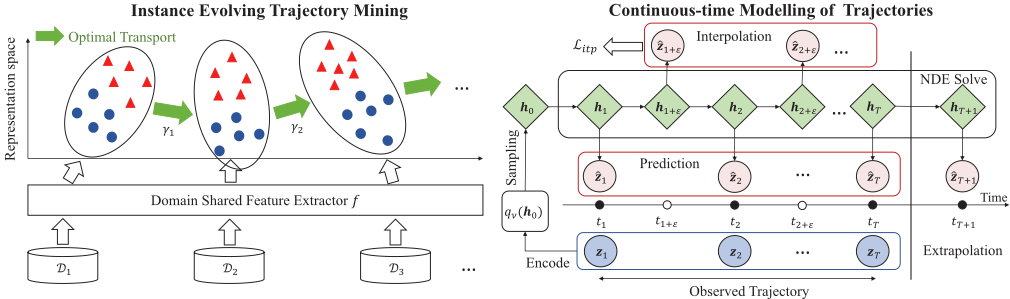
In this section, we first provide the problem formulation for TDG and then introduce our proposed CTOT framework, as depicted in Figure 1. Specifically, starting with the observed source domains, CTOT first conducts a pretraining phase to obtain a shared feature extractor that transforms input features into a representation space, then it employs OT to mine instance evolving trajectories in the joint space of representation and label. Leveraging NDEs, CTOT fits the trajectories and extrapolates them into the future domain to predict the subsequent states of the instances. These predicted virtual instances assist the model in adapting its decision boundary to the future domain. The pseudo code of the overall CTOT is provided in Appendix A.2.
4.1 ProblemFormulation
In TDG, we consider prediction tasks over an input space X and an output space Y where the joint distribution P(x, y|t) evolves with time t. In the training stage, we are given T observed source domains D1,D2, . . . ,DT sampled from data distributions on T arbitrary timestamps t1 ≤ t2 ≤ . . . ≤ tT , with each Ds = {(xis , yis ) ∼ P(x, y|ts)}ns i=1 , s = 1, 2, . . . , T where xis ∈ X, yis ∈ Y, ns denote the instance feature, label and sample size at timestamp ts, respectively. The goal of TDG is to learn a model which can generalize well on some target domain in the near future, i.e., DT+1. Note that the model is only tested once on time tT+1, differing from the online learning setting where regret is computed incrementally. Following existing TDG works [Nasery et al., 2021; Qin et al., 2022; Bai et al., 2023], we further make a necessary assumption that the joint distribution P(x, y|t) drifts smoothly over time following some underlying but unknown patterns. The main challenge of TDG is to characterize the evolving patterns of data distribution and achieve generalization using the learned evolving patterns. In the next two subsections, we will detail the two key components of CTOT: instance evolving trajectory mining and continuoustime modelling of instance evolving trajectories.
4.2 Instance Evolving TrajectoryMining
Our key insight is that capturing the instance-level evolving processes would be better suited for various complex or irregular data distributions, providing us with finer-grained information on how the decision boundary changes. For example, in influenza outbreak event prediction via Twitter [Zhao, 2023], where the task involves utilizing the counts of specific keywords across all tweets in a given region and the goal is to predict whether there will be an influenza outbreak in that region during the next week, we can get access to the information of the same region at different timestamps. However, in the case of TDG, there are no ground truth instance-toinstance correspondences between domains, or different temporal domains Ds may comprise unrelated instances (xis , yis ) without inherent correspondences. Therefore, such instance evolving trajectories do not naturally exist. To tackle the challenge, we propose to utilize OT as a principled way to seek instance-to-instance correspondences between domains and construct the instance evolving trajectories to facilitate the learning of temporal evolving patterns.
Specifically, in the context of deep learning, a model is usually composed of a feature extractor f : X → Z which maps from the original input space X to a representation space Z, and a task head g : Z → Y which outputs predictions to accomplish the task, such as classification and regression. Compared to the input space, the representation space typically exhibits advantages such as higher discriminability, lower dimensionality and better adaptability to downstream tasks through training. For these reasons, we choose to conduct instance evolving trajectory mining in the product space of representation and label, i.e., Z × Y, rather than X × Y. To obtain such a representation space, we pretrain a domainshared feature extractor f and equip each domain s with its domain-specific task head gs to accommodate the concept drift [Lu et al., 2018]. The f and {gs}Ts=1 are jointly trained on all source domains with the pretraining loss:
where ℓtask denotes the loss function associated with a specific task, which can be cross entropy loss for classification or mean-squared-error for regression. As discovered in [Gulrajani and Lopez-Paz, 2021], even in the presence of covariate shift across domains, feature extractors trained using empirical risk minimization (ERM) on mixed source domains exhibit good domain generalization capabilities if the number of source domains is sufficient. Therefore, we expect that after pretraining, f can extract features for completing the prediction task and can generalize well to the target domain.
Then, we encode each instance xis with the frozen feature extractor f to get its representation zis = f(xis ). We construct instance-to-instance correspondences between adjacent source domains by minimizing the transportation cost between them. Let µs be the empirical joint distributions of domain s over the space Ω = Z × Y, which is:
where δz,y is the Dirac function located at (z, y). We apply the Kantorovich formulation (Eq. (3)) to this discrete case to search the optimal transport plan γs between the distributions of domain s and domain s + 1, which is given by:
where ⟨·, ·⟩F denotes the Frobenius dot product, and ∆s is the transportation polytope of nonnegative matrices between two uniform distributions with dimensions ns and ns+1, i.e.,
and C ≥ 0 is the cost function matrix whose term C(i, j) = c(zis , yis , zjs+1 , yjs+1 ) denotes the transportation cost between instance (zis , yis ) and (zjs+1 , yjs+1 ). In this paper, we use a specific form of joint cost which separately considers the distance between representations and the discrepancy between labels: c(zi , yi , zj , yj ) = d(zi , zj ) + αdl(yi , yj ). Following [Damodaran et al., 2018], the distance d is chosen as squared Euclidean distance d(zi , zj ) = ∥zi -zj ∥22 . For classification, we choose the label discrepancy dl to be cross-entropy, which means the distance is 0 for instances of the same class and infinite for instances of different classes. For regression, we choose dl to be squared-loss, i.e., dl(yi , yj ) = ∥yi - yj ∥2 . The scalar α is a parameter weighting the contributions of the two terms. Convergence speedup techniques such as entropic regularization [Cuturi, 2013] are compatible with our framework and we omit it for simplicity of notation. For each instance (zis , yis ) at timestamp ts, we take the the instance (zjs+1 , yjs+1 ) at ts+1 with the maximum transportation probability in solution of Eq. (8), as its subsequent state to form instance-to-instance correspondence,i.e.,
and the value of γs[i, j] can be treated as the confidence of this correspondence relationship. We build instance-toinstance correspondences as Eq. (10) for each pair of adjacent domains, thus obtaining multiple complete instance evolving trajectories from timestamp t1 to tT , denoted by Dtra = {(zis , yis , ts)s=T s=1 }Ni=1 . Note that in practice, there may be an imbalance in the number of instances among source domains. To avoid information loss, we construct correspondences simultaneously in both forward and backward directions from the domain with the largest number of instances and obtain totally N = max{n1, n2, . . . , nT } trajectories.
4.3 Continuous-time Modelling of Trajectories
After obtaining the instance evolving trajectories Dtra, we choose to use NDEs to model them in continuous time for these reasons: (1) They offer the flexibility to handle irregularly-sampled time series, and in TDG there may be irregular time intervals between the sampled timestamps {ts}Ts=1 . (2) They are suitable for modelling continuous dynamics, and in TDG we assume the data distribution drifts smoothly following some underlying continuous dynamics. (3) They exhibit stronger extrapolation capabilities than recurrent neural networks (RNNs), especially when observations are sparse [Rubanova et al., 2019]. Note that there are other advanced continuous-time modelling approaches based on stochastic process [Deng et al., 2020; Schirmer et al., 2022; Biloˇs et al., 2023], we leave them for future work and focus only on NDEs in this paper. Specifically, we follow the latent variable time series model proposed in [Chen et al., 2018], where the generative model is defined by an NDE:
where θ denotes all the learnable parameters of the model, hs is the latent state with its initial state h0 sampled from a prior , and the dynamic of hs is governed by an NDE. ψθ is an encoder which generates the observations. For classification, we learn an NDE for each class separately to model the evolving dynamic of the representations zs within that category (We only include one NDE in Eq. (12) to keep the notation simple). For regression, we learn a single NDE which models the evolving dynamic of the concatenation of zs and ys. More detailed formulas are provided in Appendix A.1.
The model is trained to fit the trajectory data Dtra using a variational autoencoder framework [Chen et al., 2018; Li et al., 2020]. We compute the approximate posterior based on a trajectory of observations {zs, ys, ts}Ts=1 (omit the superscript i for simplicity) as:
where mh0 and vh0 are the mean and variance of the posterior, which are parameterized by some neural networks with parameters ν. Abbreviate the posterior as qν , the optimization objective is to maximize the evidence lower bound (ELBO):
To avoid the degenerated dynamics caused by unlimited temporal drift, we propose a regularization term that constrains smooth distribution shifts between two timestamps. Specifically, we interpolate some timestamps ts+ϵ (0 < ϵ < 1) between ts and ts+1, and generate the virtual instance (ˆzs+ϵ, ˆ ys+ϵ) at ts+ϵ according to Eq. (11) to Eq. (13). Since it represents the instance evolved up to time ts+ϵ, we use a weighted ensemble of the domain-specific task heads gs and gs+1, with 1 - ϵ and ϵ as weights respectively, to make prediction for the interpolated instance:
which is then regularized by the prediction loss w.r.t. the task:
The rationale here lies in the fact that the domain-specific task head gs reflects the conditional distribution p(y|z) of that domain, and we attempt to learn evolving patterns that exhibit smoothness over time, ensuring limited temporal drift within any given short time interval. Overall, the optimization objective is maximizing Eq. (15) while minimizing Eq. (17), with two hyperparameters λkl and λitp controlling the trade-off of the KL term and the interpolation loss, respectively.
Finally, we extrapolate the learned NDE dynamic of latent state into the future tT+1 to collect a set of virtual instances ˆDT+1 = {(ˆziT+1 , ˆ yiT+1 )}Ni=1 . They are used to adapt the model's decision boundary to the future to make predictions for the real test domainDT+1. In classification tasks, for each class k, we use kernel density estimation [Terrell and Scott, 1992] to estimate the conditional distribution p(z|y = k), and use time series forecasting methods to predict the prior p(y = k). The classification is performed using Bayes' rule:
In regression tasks, we fit a regression model based on the virtual representations and labels. More detailed descriptions are provided in Appendix A.3.
| Method | Classification (%) | Regression | |||||
|---|---|---|---|---|---|---|---|
| 2-Moons | Rot-MNIST | ONP | Shuttle | Elec2 | House | Appliance | |
| Offline | 22.4±4.6 | 18.6±4.0 | 33.8±0.6 | 0.77±0.10 | 23.0±3.1 | 11.0±0.36 | 10.2±1.1 |
| LastDomain | 14.9±0.9 | 17.2±3.1 | 36.0±0.2 | 0.91±0.18 | 25.8±0.6 | 10.3±0.16 | 9.1±0.7 |
| IncFinetune | 16.7±3.4 | 10.1±0.8 | 34.0±0.3 | 0.83±0.07 | 27.3±4.2 | 9.7±0.01 | 8.9±0.5 |
| CDOT [Ortiz-Jimenez et al., 2019] | 9.3±1.0 | 14.2±1.0 | 34.1±0.0 | 0.94±0.17 | 17.8±0.6 | - | - |
| CIDA [Wang et al., 2020a] | 10.8±1.6 | 9.3±0.7 | 34.7±0.6 | DNC | 14.1±0.2 | 9.7±0.06 | 8.7±0.2 |
| GI [Nasery et al., 2021] | 3.5±1.4 | 7.7±1.3 | 36.4±0.8 | 0.29±0.05 | 16.9±0.7 | 9.6±0.02 | 8.2±0.6 |
| LSSAE [Qin et al., 2022] | 9.9±1.1 | 9.8±3.6 | 38.8±1.1 | 0.22±0.01 | 16.1±1.4 | - | - |
| DDA [Zeng et al., 2023] | 9.7±1.5 | 7.6±0.7 | 34.0±0.3 | 0.21±0.02 | 12.8±1.1 | 9.5±0.12 | 6.1±0.1 |
| DRAIN [Bai et al., 2023] | 3.2±1.2 | 7.5±1.1 | 38.3±1.2 | 0.26±0.05 | 12.7±0.8 | 9.3±0.14 | 6.4±0.4 |
| EvoS [Xie et al., 2023] | 3.0±0.4 | 7.3±0.6 | 35.4±0.2 | 0.23±0.01 | 11.8±0.5 | 9.8±0.10 | 7.2±0.1 |
| CTOT (ODE) | 1.5±0.6 | 6.8±0.2 | 33.8±0.3 | 0.19±0.03 | 10.6±1.8 | 8.7±0.08 | 5.4±0.8 |
| CTOT (SDE) | 2.0±1.2 | 6.7±0.2 | 33.3±0.4 | 0.19±0.01 | 10.2±1.7 | 8.6±0.09 | 5.1±0.4 |
5 Experiments
In this section, we conduct extensive experiments to demonstrate the effectiveness of CTOT, including baseline comparisons (Section 5.2), ablation studies (Section 5.3) and hyperparameter sensitivity analysis (Section 5.4).
5.1 Experimental Settings
Datasets. Following existing works [Nasery et al., 2021; Bai et al., 2023], we conduct experiments on the following five classification datasets: Rotated Moons (2-Moons), Rotated MNIST (Rot-MNIST), Online News Popularity (ONP), Shuttle, and Electrical Demand (Elec2); and the following two regression datasets: House prices dataset (House), Appliances energy prediction dataset (Appliance). The first two datasets are synthetic, where the rotation angle serves as a proxy for time. The remaining datasets are real-world datasets with temporally evolving characteristics. More dataset details can be found in Appendix B.1.
Comparison Methods. We compare CTOT against three group of baseline methods. Time-Agnostic Baselines: These methods do not consider the temporal drift, including Offline (train on all source domains), LastDomain (train on the last source domain) and IncFinetune (sequentially train on each source domain). Continuous Domain Adaptation: CDOT [Ortiz-Jimenez et al., 2019] and CIDA [Wang et al., 2020a]. Temporal Domain Generalization: GI [Nasery et al., 2021], LSSAE [Qin et al., 2022], DDA [Zeng et al., 2023], DRAIN [Bai et al., 2023] and EvoS [Xie et al., 2023]. More baseline details can be found in Appendix B.2.
Implementation Details. To ensure a fair comparison, the network architectures for the feature extractor and task head are kept the same across all the compared methods, as employed in [Nasery et al., 2021; Bai et al., 2023]. For tuning hyperparameters, we consider data from the last source domain (DT ) as the validation set. We control the number of generated instances to be close to the number of instances in a single source domain. For each method, the experiments are repeated 5 times with different random seeds, and we report the mean results and standard deviation. More details are given in Appendix B.3 and B.4.
5.2 Performance Comparisons
Table 1 shows the comparative results of test performance on the target domain. As shown, CTOT outperforms all the baselines on the seven datasets. Additionally, we observe that CTOT with SDE demonstrates superior performance than CTOT with ODE on five of the seven datasets. This improvement is attributed to the injected noise term in an SDE, which reflects the stochasticity in the latent dynamics and the uncertainty of the instance evolving trajectories, thereby enhancing generalization. It is worth noting that the ONP dataset is exceptional, which has been shown by [Nasery et al., 2021; Bai et al., 2023] to not exhibit a strong temporal distribution shift. Therefore, the performance of all TDG baselines on ONP cannot surpass that of the time-agnostic Offline method. However, CTOT outperforms Offline on ONP, demonstrating our approach's effectiveness in capturing both time-invariant information and temporal evolving patterns. Furthermore, CTOT is applicable for both classification and regression tasks, whereas some baselines, including CDOT and LSSAE, are only suitable for classification. These results demonstrate the effectiveness and generality of CTOT. We also provide a qualitative analysis which visualizes the decision boundary predicted by CTOT in Appendix B.5.
5.3 Ablation Studies
To verify the effectiveness of all components of CTOT, we conduct ablation studies on three datasets including 2-Moons, Elec2 and House. The results are shown in Table 2.
Effect of optimal transport. To verify the effectiveness of mining instance evolving trajectories through OT, we compare CTOT with two variants: (1) CT+R, where the trajectories are constructed by randomly matching instances between each pair of adjacent domains, and (2) CT+N, where for each instance, we select the one in the next domain that is nearest to it in representation space, constructing the trajectory accordingly. As shown in Table 2, the performance of these two variants is comparatively poorer. This implies that constructing instance correspondences using a naive approach is difficult to accurately reflect the temporal trends, while OT has a stronger ability to align distributions by minimizing the global transportation cost.
| Ablation | OT | Time Model | w/ Litp | Classification (%) | Regression | |
|---|---|---|---|---|---|---|
| 2-Moons | Elec2 | House | ||||
| CT+R | × (Random) | ODE | ✓ | 7.1±3.0 | 18.4±8.7 | 9.6±0.33 |
| CT+N | × (Nearest) | ODE | ✓ | 25.3±0.8 | 19.4±9.1 | 9.3±0.26 |
| RNN+OT | ✓ | RNN | × | 3.5±1.4 | 16.2±0.6 | 9.3±0.32 |
| CTOT- | ✓ | ODE | × | 3.0±1.0 | 14.8±0.8 | 9.0±0.22 |
| CTOT | ✓ | ODE | ✓ | 1.5±0.6 | 10.6±1.8 | 8.7±0.08 |
Effect of continuous-time modelling. We further compare CTOT with two variants: (1) RNN+OT, where we employ an RNN model to fit the trajectory data and predict future data, and (2) CTOT-, where the interpolation loss Litp is not applied. We observe from Table 2 that the performance of RNN+OT is worse than CTOT-, and both are inferior to CTOT. As elaborated in [Rubanova et al., 2019], standard RNNs perform worse when observations are sparse and exhibit limited extrapolation capabilities compared to continuous-time models. Besides, applying the interpolation loss helps the model learn smoother temporal dynamics, leading to the generation of higher-quality extrapolated instances.
5.4 Hyperparameter Sensitivity Analysis
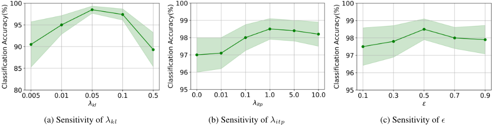
In this section, we study the effects of some key hyperparameters in our method, including the KL loss coefficient λkl, interpolation loss coefficient λitp, and interpolation point ϵ. We vary these hyperparameters and report the average and the standard deviation of the accuracy with five different random seeds on 2-Moons dataset using CTOT with ODEs.
The results of λkl are shown in Figure 2a. The curve exhibits a bell shape, which means that small λkl might result in a significant gap between the prior and posterior, impacting the quality of generated instances and large λkl might hinder the model from fitting the instance evolving trajectories. Overall, an appropriate KL coefficient is essential to learning the latent variable model defined in Eq. (11) to Eq. (13).
The results of λitp are shown in Figure 2b. We observe that the curve also exhibits a bell shape, indicating that too small λitp cannot effectively constrain the smooth distribution shift between time steps, while excessively large λitp might lead to overfitting on interpolated virtual instances, compromising the learning from real instance evolving trajectories.
The results of ϵ are reported in Figure 2c. It is shown that interpolation with different values of ϵ achieves high performance across a wide range. This suggests that our method is not highly sensitive to the specific value chosen for ϵ.
6 Conclusion
In this paper, we propose a CTOT framework for TDG. The key insight is to capture temporal evolving patterns at the instance level rather than relying on the collective behaviors of instances. The proposed CTOT framework involves two components: instance evolving trajectory mining by optimal transport and continuous-time modelling of trajectories. To facilitate the learning of continuous-time dynamics, we also introduce a novel interpolation loss which avoids the degeneration caused by unlimited temporal drift. Extensive experiments on multiple benchmark datasets demonstrate the effectiveness of CTOT compared with state-of-the-art methods.
Ethical Statement
There are no ethical issues.
Acknowledgments
This work was supported by the National Natural Science Foundation of China (U23A20468). L. Ma was supported by the Xuzhou Scientific and Technological Projects (KC23143).
@inproceedings{ijcai2024p470,
  title     = {Temporal Domain Generalization via Learning Instance-level Evolving Patterns},
  author    = {Jin, Yujie and Yang, Zhibang and Chu, Xu and Ma, Liantao},
  booktitle = {Proceedings of the Thirty-Third International Joint Conference on
               Artificial Intelligence, {IJCAI-24}},
  publisher = {International Joint Conferences on Artificial Intelligence Organization},
  editor    = {Kate Larson},
  pages     = {4255--4263},
  year      = {2024},
  month     = {8},
  note      = {Main Track},
  doi       = {10.24963/ijcai.2024/470},
  url       = {https://doi.org/10.24963/ijcai.2024/470},
}
TY - CPAPER TI - Temporal Domain Generalization via Learning Instance-level Evolving Patterns AU - Jin, Yujie AU - Yang, Zhibang AU - Chu, Xu AU - Ma, Liantao T2 - Proceedings of the Thirty-Third International Joint Conference on Artificial Intelligence, IJCAI-24 PB - International Joint Conferences on Artificial Intelligence Organization PY - 2024 SP - 4255 EP - 4263 DO - 10.24963/ijcai.2024/470 UR - https://doi.org/10.24963/ijcai.2024/470 ER -Copied
Machine-readable versions of this paper, for tools and AI agents:





