
Towards Counterfactual Fairness-aware Domain Generalization in Changing Environments
Proceedings of the Thirty-Third International Joint Conference on Artificial Intelligence. Main Track. Pages 4560-4568.
https://doi.org/10.24963/ijcai.2024/504
Keywords
- Machine Learning: ML: Causality
- AI Ethics, Trust, Fairness: ETF: Fairness and diversity
- Machine Learning: ML: Generative models
- Machine Learning: ML: Time series and data streams
Abstract
Recognizing domain generalization as a commonplace challenge in machine learning, data distribution might progressively evolve across a continuum of sequential domains in practical scenarios. While current methodologies primarily concentrate on bolstering model effectiveness within these new domains, they tend to neglect issues of fairness throughout the learning process. In response, we propose an innovative framework known as Disentanglement for Counterfactual Fairness-aware Domain Generalization (DCFDG). This approach adeptly removes domain-specific information and sensitive information from the embedded representation of classification features. To scrutinize the intricate interplay between semantic information, domain-specific information, and sensitive attributes, we systematically partition the exogenous factors into four latent variables. By incorporating fairness regularization, we utilize semantic information exclusively for classification purposes. Empirical validation on synthetic and authentic datasets substantiates the efficacy of our approach, demonstrating elevated accuracy levels while ensuring the preservation of fairness amidst the evolving landscape of continuous domains.
- [Bai et al., 2022] Guangji Bai, Chen Ling, and Liang Zhao. Temporal domain generalization with drift-aware dynamic neural networks. arXiv preprint arXiv:2205.10664, 2022.
- [Finn et al., 2017] Chelsea Finn, Pieter Abbeel, and Sergey Levine. Model-agnostic meta-learning for fast adaptation of deep networks. In International conference on machine learning, pages 1126-1135. PMLR, 2017.
- [Goodfellow et al., 2014] Ian Goodfellow, Jean Pouget- Abadie, Mehdi Mirza, Bing Xu, David Warde-Farley, Sherjil Ozair, Aaron Courville, and Yoshua Bengio. Gen- erative adversarial nets. Advances in neural information processing systems, 27, 2014.
- [Grari et al., 2021] Vincent Grari, Sylvain Lamprier, and Marcin Detyniecki. Fairness without the sensitive at- tribute via causal variational autoencoder. arXiv preprint arXiv:2109.04999, 2021. IJCAI
- [Hernán and Robins, 2018] Miguel A Hernán and James M Robins. Causal inference. International encyclopedia of statistical science, pages 1-10, 2018.
- [Hitchcock and Pearl, 2001] C. Hitchcock and J. Pearl. Causality: Models, reasoning and inference. Philosoph- ical Review, 110(4):639, 2001.
- [Hochreiter and Schmidhuber, 1997] Sepp Hochreiter and Jürgen Schmidhuber. Long short-term memory. Neural computation, 9(8):1735-1780, 1997.
- [Ilse et al., 2020] Maximilian Ilse, Jakub M Tomczak, Chris- tos Louizos, and Max Welling. Diva: Domain invariant variational autoencoders. In Medical Imaging with Deep Learning, pages 322-348. PMLR, 2020.
- [Kim and Mnih, 2018] Hyunjik Kim and Andriy Mnih. Dis- entangling by factorising. In International Conference on Machine Learning, pages 2649-2658. PMLR, 2018.
- [Kim et al., 2021] Hyemi Kim, Seungjae Shin, JoonHo Jang, Kyungwoo Song, Weonyoung Joo, Wanmo Kang, and Il- Chul Moon. Counterfactual fairness with disentangled causal effect variational autoencoder. In Proceedings of the AAAI Conference on Artificial Intelligence, volume 35, pages 8128-8136, 2021.
- [Kingma and Welling, 2013] Diederik P Kingma and Max Welling. Auto-encoding variational bayes. arXiv preprint arXiv:1312.6114, 2013.
- [Kohavi and others, 1996] Ron Kohavi et al. Scaling up the accuracy of naive-bayes classifiers: A decision-tree hy- brid. In Kdd, volume 96, pages 202-207, 1996.
- [Kusner et al., 2017] Matt J Kusner, Joshua Loftus, Chris Russell, and Ricardo Silva. Counterfactual fairness. Ad- vances in neural information processing systems, 30, 2017.
- [Louizos et al., 2017] Christos Louizos, Uri Shalit, Joris M Mooij, David Sontag, Richard Zemel, and Max Welling. Causal effect inference with deep latent-variable models. Advances in neural information processing systems, 30, 2017.
- [Miller, 2020] Jennifer Miller. Is an algorithm less racist than a loan officer? The New York Times, 2020.
- [Pearl and Mackenzie, 2018] Judea Pearl and Dana Macken- zie. The book of why: the new science of cause and effect. Basic books, 2018. [Pearl, 2009] Judea Pearl. Causality. Cambridge University Press, 2009.
- [Pfohl et al., 2019] Stephen R Pfohl, Tony Duan, Daisy Yi Ding, and Nigam H Shah. Counterfactual reasoning for fair clinical risk prediction. In Machine Learning for Healthcare Conference, pages 325-358. PMLR, 2019.
- [Qin et al., 2022] Tiexin Qin, Shiqi Wang, and Haoliang Li. Generalizing to evolving domains with latent structure- aware sequential autoencoder. In International Conference on Machine Learning, pages 18062-18082. PMLR, 2022.
- [Qin et al., 2023] Tiexin Qin, Shiqi Wang, and Haoliang Li. Evolving domain generalization via latent structure-aware sequential autoencoder. IEEE Transactions on Pattern Analysis and Machine Intelligence, 2023.
- [Shpitser and Pearl, 2008] Ilya Shpitser and Judea Pearl. Complete identification methods for the causal hierar- chy. Journal of Machine Learning Research, 9:1941- 1979, 2008.
- [Sohn et al., 2015] Kihyuk Sohn, Honglak Lee, and Xinchen Yan. Learning structured output representation using deep conditional generative models. Advances in neural infor- mation processing systems, 28, 2015.
- [Spirtes et al., 2000] Peter Spirtes, Clark N Glymour, Richard Scheines, and David Heckerman. Causation, prediction, and search. MIT press, 2000.
- [Wang et al., 2021] Yufei Wang, Haoliang Li, Lap-Pui Chau, and Alex C Kot. Variational disentanglement for domain generalization. arXiv preprint arXiv:2109.05826, 2021.
- [Wang et al., 2022] William Wei Wang, Gezheng Xu, Ruizhi Pu, Jiaqi Li, Fan Zhou, Changjian Shui, Charles Ling, Christian Gagné, and Boyu Wang. Evolving domain gen- eralization. arXiv preprint arXiv:2206.00047, 2022.
- [Wu et al., 2019] Yongkai Wu, Lu Zhang, Xintao Wu, and Hanghang Tong. Pc-fairness: A unified framework for measuring causality-based fairness. Advances in neural information processing systems, 32, 2019.
- [Zafar et al., 2017] Muhammad Bilal Zafar, Isabel Valera, Manuel Gomez Rogriguez, and Krishna P Gummadi. Fair- ness constraints: Mechanisms for fair classification. In Ar- tificial intelligence and statistics, pages 962-970. PMLR, 2017.
- [Zeng et al., 2023] Qiuhao Zeng, Wei Wang, Fan Zhou, Charles Ling, and Boyu Wang. Foresee what you will learn: Data augmentation for domain generaliza- tion in non-stationary environments. arXiv preprint arXiv:2301.07845, 2023.
- [Zhao and Chen, 2020] Chen Zhao and Feng Chen. Un- fairness discovery and prevention for few-shot regression. In 2020 IEEE International Conference on Knowledge Graph (ICKG), pages 137-144. IEEE, 2020.
- [Zhao et al., 2021a] Chen Zhao, Feng Chen, and Bhavani Thuraisingham. Fairness-aware online meta-learning. In Proceedings of the 27th ACM SIGKDD Conference on Knowledge Discovery & Data Mining, pages 2294-2304, 2021.
- [Zhao et al., 2021b] Tianxiang Zhao, Enyan Dai, Kai Shu, and Suhang Wang. You can still achieve fairness with- out sensitive attributes: Exploring biases in non-sensitive features. arXiv preprint arXiv:2104.14537, 2021.
- [Zhao et al., 2022] Chen Zhao, Feng Mi, Xintao Wu, Kai Jiang, Latifur Khan, and Feng Chen. Adaptive fairness- aware online meta-learning for changing environments. In Proceedings of the 28th ACM SIGKDD Conference on Knowledge Discovery and Data Mining, pages 2565- 2575, 2022.
- [Zhao et al., 2023] Chen Zhao, Feng Mi, Xintao Wu, Kai Jiang, Latifur Khan, Christan Grant, and Feng Chen. To- wards fair disentangled online learning for changing envi- ronments. In Proceedings of the 29th ACM SIGKDD Con- ference on Knowledge Discovery and Data Mining, pages 3480-3491, 2023.
References were extracted automatically from the PDF and may contain errors.
Full text extracted automatically from the PDF; figures, tables and equations may differ. The PDF is the version of record.
1 Introduction
The distribution shifts across sequential data domains drive the need for machine learning models with evolving domain generalization capabilities [Wang et al., 2022]. It requires the development of models in learning invariant representations across distinct temporal periods, consequently enhancing generalization to evolving data distributions. The temporal alignment between source and target domains [Zeng et al., 2023] contributes to adaptive machine learning solutions, which prove indispensable in dynamic environments or evolving data streams.
∗This paper is supervised by Chen Zhao and Minglai Shao.
†Corresponding author.
As methodologies extend domain generalization to continuously evolving environments, there is a tendency to prioritize accuracy, neglecting equitable model treatment across novel domain sequences. Fairness, a significant concern in machine learning, cannot be disregarded. Sensitive features, containing protected information, include attributes like race, gender, religion, or socioeconomic status, safeguarded by ethical considerations, legal regulations, or societal norms. For instance, during the COVID-19 pandemic, systemic algorithms exhibited discrimination against African American individuals in bank loans [Miller, 2020]. Causal models have been widely applied in machine learning to address issues related to model fairness. Structural Causal Models (SCMs) [Hitchcock and Pearl, 2001] provide a means of explaining machine learning model predictions. Analyzing causal graphs and paths helps understand how the model's predictions for different groups are formed, thereby identifying and addressing potential unfair factors. Simultaneously, to analyze fairness based on SCMs, a concept known as counterfactual fairness [Kusner et al., 2017] has been introduced. This concept seeks to minimize the impact on predicted values when counterfactual interventions are applied to sensitive attributes. In the context of dynamically evolving environments, we propose a framework, denoted as Disentanglement for Counterfactual Fairness-aware Domain Generalization (DCFDG), designed to address the issue of counterfactual fairness.
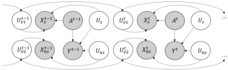
Our objective can be succinctly summarized as aiming to enhance the model's generalization capacity across unfamiliar domain sequences while concurrently ensuring counterfactual fairness in decision-making. Therefore, to model the relationships among sensitive attributes, domain-specific information, and semantic information, we partition the exogenous variables into four latent variables: 1) semantic information caused by sensitive attributes: Us, 2) semantic information not caused by sensitive attributes: Uns, 3) domainspecific information caused by sensitive attributes: Uv1, and 4) domain-specific information not caused by sensitive attributes: Uv2. Among these, we posit that the distribution of semantic information remains invariant across all domains, whereas the distribution of domain-specific information varies with changes in the environment. Here, the data feature X is composed of two components, wherein sensitive attribute A directly causes a subset of features (Xs), while another subset of features (Xns) is not directly influenced by A but may still exhibit correlations with it. They are encoded in the latent space as the first two exogenous variables (i.e., Us and Uns). The advantages of this partitioning will be elucidated in the causal structure of DCFDG (Section 4.1). By employing such an approach, we skillfully disentangle domainspecific information (i.e., Uv1 and Uv2) from the embedded representation of classification features, ensuring a reduction in the impact of environmental changes on the model while concurrently upholding its decision fairness. In conclusion, our contributions can be summarized as follows:
- We introduce a novel causal structure framework, DCFDG, which adeptly addresses data distributions that evolve within dynamic environments and are influenced by sensitive information. To the best of our knowledge, this is the first method of addressing counterfactual fairness issues in dynamic evolving environments.
- We analyze the Evidence Lower Bound (ELBO) that should be considered within evolving environments. Besides, we theoretically demonstrate the rationality of DCFDG.
- Experimental results conducted on both synthetic and realworld datasets demonstrate that DCFDG exhibits superior predictive capabilities compared to existing exogenous variable disentanglement methods, while concurrently ensuring fairness.
2 RelatedWork
Domain Generalization in Changing Environments. To address the generalization issues in continuously changing environments, Bai et al. [2022] involve passing the parameters of neural networks into a temporal encoder to train domain-specific parameters for each different domain. Another approach is to separately model environmental information in both features and labels, enabling the simultaneous handling of covariate shift and concept shift [Qin et al., 2022]. Zeng et al. [2023] explore aligning the data distribution in the training domain with that in an unseen domain as a means of addressing these challenges. Additionally, a classic work proposed a model-agnostic meta-learning (MAML) algorithm that learns to adapt quickly to new domains, demonstrating its effectiveness in few-shot domain generalization [Finn et al., 2017]. Building upon this work, Zhao et al. [2021a; 2022; 2023] introduces a method that incorporates fairness considerations.
Counterfactual Fairness with Variational Autoencoder. Consider X, A, Y , and U as data features, sensitive attributes, classification labels, and exogenous variables, respectively. Conditional Variational Autoencoder (CVAE) [Sohn et al., 2015] extends this framework by incorporating additional conditional information, such as labels Y , during the generation process. Louizos et al. [2017] propses a causal graph. In their CEVAE, A and X have an indirect connection through U, while A has both a direct and an indirect connection with Y simultaneously. However, this approach embeds A's information in U, rendering the counterfactual generation process of p(y|¬a, u) infeasible. To address this issue, an enhanced causal graph is proposed, assuming that X and Y are caused by both A and U [Pfohl et al., 2019]. It employs Maximum Mean Discrepancy to regularize the generations, effectively removing A's information from U. Although this approach eliminates all A-related components from U, the ideal scenario should involve the removal of only the portion in U that is caused by A, rather than all A-related components. Therefore, DCEVAE [Kim et al., 2021] is proposed to define Xs ⊂ X as a subset of features caused by A whereas Xns ⊂ X is the other subset of irrelevant features to the intervention. The intervention on A should be imposed on Xs, and Xns should be maintained in a counterfactual generation.
3 Background
3.1 Structual Causal Model and Do-operator
Structural causal models (SCMs) are widely used in causal inference to model the causal relationships among variables. An SCM consists of a directed acyclic graph (DAG) and a set of structural equations that define the causal relationships among the variables in the graph [Pearl, 2009; Spirtes et al., 2000; Pearl and Mackenzie, 2018]. The structural equation for an endogenous variable Vi can be expressed as follows:
where PaVi denotes the parent set of Vi in the graph, and UVi denotes the set of exogenous variables that directly affect Vi. The function fi represents the causal relationship between the parent variables and Vi. SCMs are used to estimate causal effects and test causal hypotheses. By including sensitive variables in the graph and modeling their causal relationships with other variables, SCMs can adjust for sensitive and produce unbiased estimates of causal effects [Hern´an and Robins, 2018].
Interventions on SCMs involve changing the value of a variable to a specified value. This can be represented mathematically using the do-operator, denoted by do(Vi = v). The do-operator separates the effect of an intervention from the effect of other variables in the system. For example, if we want to investigate the effect of drug treatment on a disease outcome, we might use the do-operator to set the value of the treatment variable to "treated" and observe the effect on the outcome variable. In the following narrative, we will employ an alternative representation for the do-operator. For two variables: ˆY ,A and given exogenous variable set U,
3.2 Counterfactual Fairness Problem
Counterfactual fairness is a concept that models fairness using causal inference tools, first introduced by [Kusner et al., 2017]. Given a predictive problem with fairness considerations, where A, X, Y , and ˆ Y represent the sensitive attributes, remaining attributes, the output of interest, and model estimation respectively. A SCM G := ⟨U, V, F, P(u)⟩ is given, where V is the set of endogenous variables, P(v) := P(V = v) = ∑{u|fV (V,u)=v} P(u), and U is the set of exogenous variables. the set of deterministic functions F is defined in Vi = fVi (PaVi ,UVi ) like Eq.1. We can say predictor ˆ Y is counterfactually fair, if
for all y and any value ¬a attainable by A. By setting A to both a and ¬a separately, ˆ Y evolves into two distinct variants: ˆ YA←a and ˆ YA←¬a. From an intuitive perspective, counterfactual fairness seeks to ensure that the values of sensitive attribute A do not influence the distribution of predicted outcome ˆ Y .
3.3 Counterfactual Fairness in Evolving Environments
We consider classification tasks where the data distribution evolves gradually with time. In training stage, we are given T sequentially arriving source domains S = {D1, D2, ..., DT }, where each domain Dt = {(xti , ati , yt i )}nt i=1 is comprised of nt labeled samples for t ∈ {1, 2, ..., T}. And x, a, and y denote the data features, the sensitive label, and the class label respectively. The trained model will be tested on M target domains T = {DT+1,DT+2, ...,DT+M}, Dt = {(xti , ati , yt i )}nt i=1 (t ∈ {T +1, T +2, ..., T +M}), which are not available during training stage. For simplicity, we omit the index i whenever xti refers to a single data point. Our primary objective is to enhance the robustness of the model on these unseen domains to achieve higher accuracy. Meanwhile, we are also committed to ensuring classification fairness across these M target domains, resulting in the following expression for Eq.3:
4 Methodology
In this section, we will introduce the causal structure of our model. Building upon this causal structure, we will further elaborate on the entire training process of the model, including the formulation of the loss function used.
4.1 Causal Structure of DCFDG
The causal graph depicting two consecutive domains is illustrated in Fig. 1. To achieve the counterfactual generation of p(y|¬a, u) for intervention on A, it is crucial to ensure that the exogenous variable U does not contain any part caused by A. Otherwise, there will be situations where intervention on A occurs, but the information caused by A in U remains unchanged, leading to an erroneous generation of y. To address the problem, we define Xs ⊂ X as a subset of features caused by A, whereas Xns ⊂ X is the other subset of irrelevant features to the intervention. This is a common method of partitioning features in the context of fairness issues [Zhao et al., 2021b; Grari et al., 2021; Kim et al., 2021]. For instance, considering the 'Sex' attribute in the Adult dataset as the sensitive attribute, we can broadly describe the characteristics of this attribute as Xs = {Occupation,Workclass, ...}, while the remaining features can be denoted as Xns. Similarly, let's define the exogenous variables of Xns and Xs to be Uns and Us, respectively. We assume that Us and Uns are disentangled. Ideally, Us contains the portion caused by A, rather than the part correlated with A. Therefore, we need to disentangle Us from A. On the other hand, Uns contains only the part correlated with A and does not require decoupling from A. However, in the face of a constantly changing environment, it becomes imperative to devise strategies for decoupling the domain-specific information from Xs and Xns. To simulate dynamic environments, we adopt two variables, Uv1 and Uv2, to capture the dynamic changes in the distributions of Xs and Xns respectively, as they vary with the environments. For the domain Dt at timestamp t, we represent Uv1 and Uv2 as U t v1 and U t v2 , respectively.
4.2 Network Architecture of DCFDG
Based on our causal graph, the corresponding neural network architecture is shown in Fig. 2, encompassing both the inference and generation processes. During the inference stage, we employ four distinct encoders to model q(us|xts , at ), q(uns|xtns ), q(uv1|xts ) and q(uv2|xtns ), respectively. The prior distributions for us and uns follow standard normal distributions. For the environmental variable sequences {U t v1 }Tt and {U t v2 }Tt , we can regard them as two temporal priors (i.e., p(utv1 ) = p(utv1 |u<t v1 ) and p(utv2 ) = p(utv2 |u<t v2 )). Hence, all the prior distributions are as follows:
where the distribution p(utv1 |u<t v1 ) and p(utv2 |u<t v2 ) can be encoded using recurrent neural networks such as LSTM [Hochreiter and Schmidhuber, 1997]. Wherein, at the initial state when t = 0, u0v1 and u0v2 is initialized to 0. In the generation phase, all latent variables are fed into two distinct decoders and a classifier to reconstruct Xs, Xns, and Y . To enhance adaptability within a dynamically changing environment, we solely utilize environment-independent semantic information to reconstruct Y .
4.3 Evidence Lower Bound of DCFDG
For any given time point t and domain Dt = {(xti , ati , yt i )}nt i=1 , we employ Us and Uns to capture the invariant semantic information within the distribution, while U t v1 and U t v2 are utilized to encapsulate the domain-relevant information. Analogous to the Variational Autoencoder (VAE) [Kingma and Welling, 2013], in this context, q denotes the inference process, while p signifies the generation process. The detailed derivation process of the ELBO for DCFDG is provided in Appendix A.5.
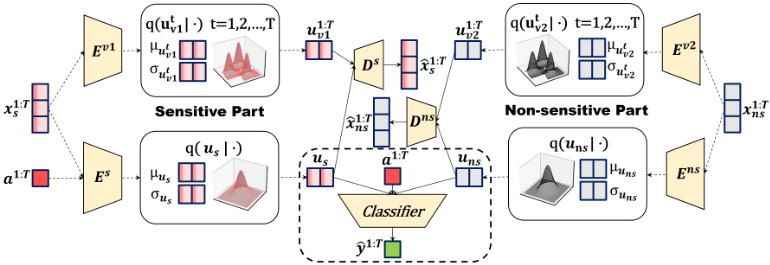
Sensitive Part. To encode representations containing sensitive information, we employ the sensitive attribute A to contribute to the encoding process. Therefore, the ELBO of the sensitive part can be represented as follows:
Non-sensitive Part. Like the sensitive part, the ELBO of the non-sensitive part can be represented as follows:
Prediction Generation. We use semantic representations and sensitive attributes for classification and the loss is:
Final ELBO of DCFDG. Taking into account the three aforementioned components, we derive the final ELBO as follows:
During the training process, it is imperative to maximize this ELBO, consequently rendering its negative counterpart, the -ELBO , a constituent of the objective function.
4.4 Counterfactual Fairness Loss of DCFDG
The essence of counterfactual fairness lies in minimizing the impact of A on the predicted value ˆ Y . Therefore, for our model, if the condition:
is satisfied, the model's predictions attain complete counterfactual fairness in such a case. To earnestly achieve fairness in classification, it is imperative to augment the objective function with a fairness regularization term:
where for the sake of simplicity, every attribute A is treated as a binary variable in this paper, and ¬a denotes the negation of its original value.
4.5 Adversarial Loss of DCFDG
Building upon the analysis of causal structure, Us is concurrently disentangled from both A and Uns. In other words, Us is simultaneously independent of both A and Uns (i.e., q(us, at , uns) = q(us)q(at , uns)). Hence, the disentanglement objective is equivalent to minimizing the KL divergence between q(us, at , uns) and q(us)q(at , uns). However, computing this KL divergence directly is infeasible, prompting us to leverage an approach akin to the one proposed in FactorVAE [Kim and Mnih, 2018], which bears resemblance to GAN-like [Goodfellow et al., 2014] principles, to address this challenge. We begin by employing a discriminator D, which outputs a probability that a set of samples originates from the distribution q(us, at , uns) rather than q(us)q(at , uns). Hence, we can approximate the KL divergence as follows using the loss function LTC about D:
Furthermore, to train the discriminator D, we should maximize MD:
Algorithm 1 Optimization procedure for DCFDG
- 1: Input: sequential source labeled datasets S with T domains; static feature extractor Es , Ens ; dynamic inference networks Ev1 , Ev2 and their corresponding prior networks (LSTM) F v1 , F v2 ; decoder Ds , Dns ; discriminator D; classifier C.
- 2: Initialize Es ,Ens ,Ev1 ,Ev2 , F v1 , F v2 ,Ds , Dns ,D,C
- 3: Assign u0v1 , u0v2 ← 0
- 4: for t = 1, 2, ..., T do
- 5: Generate prior distribution p(utv1 |u<t v1 ) via F v1
- 6: Generate prior distribution p(utv2 |u<t v2 ) via F v2
- 7: for i = 1, 2, ... do
- 8: Sample a batch of data (xts , xtns , at , yt ) from Dt
- 9: Calculate LDCFDG by Eq. 13
- 10: Update Es , Ens ,Ev1 , Ev2 ,F v1 , F v2 ,Ds , Dns and C by LDCFDG
- 11: CalculateMD by Eq. 12
- 12: Update D byMD
- 13: end for
- 14: end for
where perm[us, at , uns] denotes the randomized alteration of the relative sequence between (at , uns) and us.
4.6 Ultimate Objective Function
We denote all parameters of DCFDG, including all encoders, decoders, and prior networks (LSTMs), as θ, and the parameters of discriminator D as ψ. Summing up the preceding sections, the training objectives of the model can be summarized into two phases as follows:
After the completion of training within the DCFDG framework (Algorithm. 1), we require the trained static feature extractor Es and Ens to obtain semantic information (us and uns). Finally, the classifier C is utilized for prediction by inputting both us and uns alongside sensitive attribute a.
5 Theoretical Guarantee of DCFDG
Due to the usual representation of ELBO as a sum of multiple terms, we delve into its equivalent optimization objective in theoretical analysis.
Lemma 1. In the vanilla VAE, the KL divergence KL(q(u|x)||p(u|x)) can be represented as
Based on Lemma 1, we can derive the Evidence Lower Bound (ELBO) of the vanilla VAE in the following formula:
It means that optimizing the ELBO of VAEs is equivalent to optimizing KL(q(u|x)||p(u|x)). We denote the samples from the source domains as X1:T s and X1:T ns , while the features of samples from the unseen target domains are represented as XT+m s and XT+m ns for m ≥ 1. The relationship between the source domains and the target domains can be expressed as follows.
Theorem 1. The KL divergence between q(us, uns|xT +m s , aT+m, xT+m ns ) and the unknown domain-invariant ground truth distribution p(us, uns|xT +m s , aT+m, , xT+m ns ) can be bounded as follows:
where x1:T,i s , a1:T,i and x1:T,i ns denotes features with index i in source domains. The feasible set I [Wang et al., 2021] and constant βi are defined in Appendix A.3. Semantic information us and uns are defined in Section 4.1.
This inequality expresses that the ELBO on the target domains can be optimized by separately optimizing the ELBO concerning Xs and Xns on the source domains. Therefore, Theorem 1 ensures that DCFDG is a rational and effective methodology. The detailed proof of Theorem 1 is provided in Appendix A.4.
6 Experiments
6.1 Datasets
FairCircle is a synthetic dataset containing 12 domains. For each domain, followed by [Zafar et al., 2017], we generate 2000 binary class labels uniformly at random and assign a two-dimensional feature vector x = [xs, xns]T per label by sampling from two distinct Gaussian distributions: P(x|y = 0) = N(µ0, [10, 1; 1, 3]) and P(x|y = 1) = N(µ1, [5, 1; 1, 5]), where µ0 and µ1 will changed by domain. Sensitive attributes of data samples are drawn from a Bernoulli distribution P(a = 1) = P(x′ |y=1) P(x′ |y=1)+P(x′ |y=0) , where x′ = [cos(ϕ),-sin(ϕ); sin(ϕ), cos(ϕ)][xs; 1] is simply a rotated vector related to xs. The ϕ controls the correlation between the sensitive attribute and the class labels. The ϕ in each domain is a random number between π8 and π4 . The closer ϕ is to zero, the higher the correlation. To construct multiple sequentially changing domains, we uniformly sampled 12 values of µ0 and µ1 from two circular arcs with radii of 25 and 34, respectively, to simulate the variation in data distribution. The visualization of the dataset is provided in Appendix B.1.
Adult [Kohavi and others, 1996] contains a diverse set of attributes pertaining to individuals in the United States. The dataset is often utilized to predict whether an individual's annual income exceeds 50,000 dollars, making it a popular choice for binary classification tasks. We categorize gender as a sensitive attribute. Income is designated as the dependent variable Y . Race, age, and country of origin constitute the set Xns, while the remaining variables comprise the set Xs [Zhao et al., 2021b; Grari et al., 2021; Kim et al., 2021]. We divided the samples into 18 domains based on age, ranging from younger to older. Specifically, the source domain tends to represent a younger demographic, while the target domain tends to represent an older demographic.
| FairCircle | Adult | Chicago Crime | ||||||||||||||
|---|---|---|---|---|---|---|---|---|---|---|---|---|---|---|---|---|
| Methods | Acc ↑ | TCE ↓ (×10) | Acc ↑ | TCE (×10) | ↓ | CE ↓ | (×10) | Acc ↑ | TCE ↓ (×10) | CE ↓ | (×10) | |||||
| o00 | o01 | o10 | o11 | o00 | o01 | o10 | o11 | |||||||||
| DIVA [Ilse et al., 2020] | 69.10 | 1.15 | 68.04 | 0.81 | 0.88 | 0.62 | 0.34 | 0.86 | 56.19 | 1.68 | 1.68 | 1.46 | 1.84 | 1.75 | ||
| LSSAE [Qin et al., 2022] | 89.25 | 5.03 | 57.79 | 1.91 | 2.96 | 3.64 | 1.70 | 1.67 | 53.72 | 0.85 | 0.77 | 0.93 | 0.90 | 0.77 | ||
| MMD-LSAE [Qin et al., 2023] | 82.79 | 0.70 | 60.34 | 1.60 | 1.17 | 1.35 | 1.05 | 1.68 | 53.83 | 0.35 | 0.23 | 0.41 | 0.36 | 0.31 | ||
| CVAE [Sohn et al., 2015] | 49.99 | 0.18 | 61.83 | 0.56 | 0.53 | 0.55 | 0.51 | 0.57 | 54.43 | 0.72 | 0.67 | 0.70 | 0.74 | 0.77 | ||
| CEVAE [Louizos et al., 2017] | 49.99 | 0.34 | 62.49 | 0.69 | 0.68 | 0.69 | 0.69 | 0.69 | 54.23 | 0.42 | 0.40 | 0.43 | 0.42 | 0.44 | ||
| mCEVAE [Pfohl et al., 2019] | 63.30 | 0.28 | 61.05 | 0.48 | 0.45 | 0.35 | 0.50 | 0.48 | 51.83 | 0.01 | 0.01 | 0.01 | 0.01 | 0.01 | ||
| DCEVAE [Kim et al., 2021] | 53.25 | 0.18 | 62.69 | 0.39 | 0.39 | 0.38 | 0.39 | 0.38 | 51.29 | 0.44 | 0.48 | 0.45 | 0.44 | 0.39 | ||
| DCFDG (Ours) | 88.70 | 0.12 | 69.85 | 0.22 | 0.10 | 0.01 | 0.17 | 0.26 | 55.93 | 0.01 | 0.01 | 0.01 | 0.01 | 0.01 | ||
Chicago Crime [Zhao and Chen, 2020] dataset includes a comprehensive compilation of criminal incidents in different communities across Chicago city in 2015. We use race (i.e., black and non-black) as the sensitive attribute. To better delineate between Xs and Xns, we measured the Pearson Product-Moment Correlation Coefficients (PPMCC) values between each feature and sensitive attribute (Appendix B.2). This was done to gauge their correlation and aid in the partitioning process. Grocery count, per capita income, aged 25+ without high school diploma, and housing crowd of origin constitute the set Xns, while the remaining variables comprise the set Xs. The dataset was collected over time, and as a result, we partition the data into 18 domains based on chronological order. The target domain consists of the most recent samples.
6.2 Baseline Methods
We evaluate the proposed DCFDG against seven baseline methods. These baselines are selected from two perspectives: approaches that utilize causal structures to tackle evolving domain generalization (DIVA [Ilse et al., 2020], LSSAE [Qin et al., 2022], and MMD-LSAE [Qin et al., 2023]), and methods that utilize causal structures to address counterfactual fairness (CVAE [Sohn et al., 2015], CEVAE [Louizos et al., 2017], mCEVAE [Pfohl et al., 2019], and DCEVAE [Kim et al., 2021]).
6.3 EvaluationMetrics
We employed two metrics, total causal effect and counterfactual effect, to evaluate the fair classification. Assuming A is the intervention target of the do-operator, Y is influenced by this intervention. The post-intervention distribution of Y mentioned in Section 3.1 can be further abbreviated as P(ya).
Definition 1 (Total Causal Effect (TCE) [Pearl, 2009]). The total causal effect of the value change of A from a to ¬a on Y = y is given by TCE(a, ¬a) = |P(ya) - P(y¬a)|.
Definition 2 (Counterfactual Effect (CE) [Shpitser and Pearl, 2008]). Given context O = o, the counterfactual effect of the value change of A from a to ¬a on Y = y is given by CE(a, ¬a|o) = |P(ya|o) - P(y¬a|o)|.
Smaller TCE and CE indicate that the prediction results are more stable in the counterfactual generation of changing the sensitive attribute, implying greater fairness [Wu et al., 2019].
For the Adult dataset, we set context of counterfactual effect as O = {race, native country}. For the Crime dataset, we set context of counterfactual effect as O = {grocery count, per capital income}. In both two datasets, oij denotes the first attribute as i and the second attribute as j.
6.4 Experimental Setup
We partitioned the domains into source, intermediary, and target domains by the ratio ( 12 : 16 : 13 ). The source domains are employed for training the DCFDG, while the intermediary domains serves as the validation set. All evaluations are conducted within the target domains. For the FairCircle dataset, direct computation of its counterfactual effect (CE) is unfeasible because its features are randomly sampled continuous numerical values. As for the other two datasets, both the total causal effect (TCE) and CE were employed for evaluation purposes. For all the encoders, decoders, classifiers, and discriminators, we employed the most common fully connected layers and ReLU activation functions. The specific architecture details can be found in Appendix B.3.
6.5 Results Analysis
Overall Performance. We computed the mean performance across all testing domains, as depicted in Table 1. Smaller values of TCE and CE indicate closer adherence of the classification outcomes to counterfactual fairness. To facilitate observation, the reported results encapsulate the values of TCE and CE across all outcomes. Across the three datasets, DCFDG consistently demonstrates favorable generalization capabilities to unknown domains compared to other approaches, achieving optimal performance. Notably, its pronounced superiority in accuracy on the FairCircle dataset is believed to stem from the discernible advantage exhibited as the data distribution between each domain varies to a greater extent. Regarding TCE and CE, DCFDG consistently achieves optimal or near-optimal outcomes. This underscores the resilience of our approach to maintaining high performance while simultaneously upholding fairness principles. For the Chicago Crime dataset, while there hasn't been a substantial improvement in decision accuracy, it is noteworthy that both its TCE and CE values are considerably lower than the highest accuracy method: DIVA. In other words, in the context of comparable accuracy levels, fairness significantly outperforms alternative methods.

| Adult | Chicago Crime | |||
|---|---|---|---|---|
| Metric | Acc ↑ | TCE ↓ (×10) | Acc ↑ | TCE ↓ (×10) |
| w/o disentanglement | 71.48 | 0.47 | 54.43 | 1.61 |
| w/o fairness loss | 72.24 | 2.76 | 54.89 | 1.75 |
| DCFDG | 69.85 | 0.22 | 55.93 | 0.01 |
Performance Across Each Domain. In Figure 3, we present the results across each testing domain. For the FairCircle dataset, there are four testing domains, while the Adult and Chicago Crime datasets have six testing domains each. The 1st, 3rd, and 5th figures represent accuracy outcomes, with higher curves indicating superior performance. The 2nd, 4th, and 6th figures illustrate TCE results, with lower curves signifying enhanced compliance with counterfactual fairness, concurrently denoted by the shaded regions representing standard deviations. Across all testing domains, DCFDG consistently maintains superior accuracy and minimal TCE values. Regarding the tabulated data encompassing the mean and standard deviation of all three metrics across each domain, we present this information uniformly within the Appendix B.6.
6.6 Ablation Study
We evaluate the effect of components in the design of DCFDG's objective. We have specifically examined two variants of DCFDG as follows.
Without Disentanglement. We attempted to refrain from decoupling features into domain-specific and semantic information, opting instead for utilizing a globally modeled dynamic Gaussian distribution for predictions. As indicated in Table 2, the absence of feature decoupling adversely impacted classification fairness, particularly evident in the Crime dataset.
Without Fairness Loss. We eliminated the loss associated with counterfactual fairness to assess changes in the outcomes. Despite achieving a marginal advantage in prediction accuracy on the adult dataset, a sharp increase in the TCE value resulted in unfair classification outcomes (Table 2).
Experimental results regarding the CE values can be found in Appendix B.4. The above experiments indicate that decoupling domain-specific information and incorporating the fairness loss are both indispensable for ensuring counterfactual fairness.
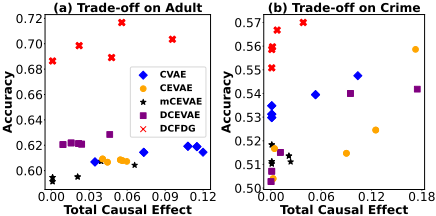
6.7 Fairness-accuracy Trade-off
Due to the absence of fairness loss in certain baselines, we compare our method with four baselines about the trade-off between accuracy and fairness on target domains under different parameters. We varied the parameter λf across five values ([0.02, 0.1, 0.2, 0.5, 1]) to obtain the results of each baseline under these five settings. In Figure 4, the horizontal axis represents TCE values, and the vertical axis represents accuracy, indicating that data points tending towards the upper-left corner exhibit superior performance. Experimental results regarding the CE values can be found in Appendix B.5. All the results demonstrate that DCFDG achieves the best overall performance.
7 Conclusion
In summary, this paper has proposed a novel framework, DCFDG, to address issues of fairness within continuously evolving dynamic environments. This method disentangles exogenous variables based on the relationships among sensitive attributes, domain-specific information, and semantic information, partitioning them into four latent variables. By leveraging these latent variables, a causal structure is constructed for our method. We establish an appropriate model and optimize the corresponding objective function through this causal graph. Theoretical analysis and experimental validation attest to the efficacy of DCFDG.
Acknowledgements
This work is supported by the National Natural Science Foundation of China program (NSFC #62272338).
@inproceedings{ijcai2024p504,
  title     = {Towards Counterfactual Fairness-aware Domain Generalization in Changing Environments},
  author    = {Lin, Yujie and Zhao, Chen and Shao, Minglai and Meng, Baoluo and Zhao, Xujiang and Chen, Haifeng},
  booktitle = {Proceedings of the Thirty-Third International Joint Conference on
               Artificial Intelligence, {IJCAI-24}},
  publisher = {International Joint Conferences on Artificial Intelligence Organization},
  editor    = {Kate Larson},
  pages     = {4560--4568},
  year      = {2024},
  month     = {8},
  note      = {Main Track},
  doi       = {10.24963/ijcai.2024/504},
  url       = {https://doi.org/10.24963/ijcai.2024/504},
}
TY - CPAPER TI - Towards Counterfactual Fairness-aware Domain Generalization in Changing Environments AU - Lin, Yujie AU - Zhao, Chen AU - Shao, Minglai AU - Meng, Baoluo AU - Zhao, Xujiang AU - Chen, Haifeng T2 - Proceedings of the Thirty-Third International Joint Conference on Artificial Intelligence, IJCAI-24 PB - International Joint Conferences on Artificial Intelligence Organization PY - 2024 SP - 4560 EP - 4568 DO - 10.24963/ijcai.2024/504 UR - https://doi.org/10.24963/ijcai.2024/504 ER -Copied
Machine-readable versions of this paper, for tools and AI agents:





