
Simple Contrastive Multi-View Clustering with Data-Level Fusion
Proceedings of the Thirty-Third International Joint Conference on Artificial Intelligence. Main Track. Pages 4697-4705.
https://doi.org/10.24963/ijcai.2024/519
Keywords
- Machine Learning: ML: Self-supervised Learning
- Machine Learning: ML: Multi-modal learning
- Machine Learning: ML: Clustering
- Machine Learning: ML: Multi-view learning
Abstract
Previous deep multi-view clustering methods usually design un-shared encoders to explore the cluster information among multi-view data, but they are difficult to customize the encoders for individual views and easily increase information loss. To address these issues, we propose a simple yet effective contrastive multi-view clustering framework. Specifically, different from using feature-level fusion in previous methods, we first propose a data-level fusion method to fuse multi-view information, which produces a fused data to replace all views and thus avoids customizing networks for different views. Then, we simulate the data noise and unavailability in multiple views to design two kinds of data augmentation for the fused data, making a shared encoder with simple contrastive learning to learn robust features and achieve the interaction across views. As a result, our method is a general framework and we base on it to conduct feature clustering and end-to-end clustering. Extensive experiments demonstrate that our method can explore the discriminative information in multi-view data and achieve superior clustering performance.
- [Abavisani and Patel, 2018] Mahdi Abavisani and Vishal M Patel. Deep multimodal subspace clustering networks. IEEE J-STSP, 12(6):1601-1614, 2018.
- [Andrew et al., 2013] Galen Andrew, Raman Arora, Jeff Bilmes, and Karen Livescu. Deep canonical correlation analysis. In ICML, pages 1247-1255, 2013.
- [Bickel and Scheffer, 2004] Steffen Bickel and Tobias Scheffer. Multi-view clustering. In ICDM, pages 19-26, 2004.
- [Cai et al., 2012] Xiao Cai, Hua Wang, Heng Huang, and Chris Ding. Joint stage recognition and anatomical an- notation of drosophila gene expression patterns. Bioinfor- matics, 28(12):i16-i24, 2012.
- [Chen et al., 2022] Man-Sheng Chen, Jia-Qi Lin, Xiang- Long Li, Bao-Yu Liu, Chang-Dong Wang, Dong Huang, and Jian-Huang Lai. Representation learning in multi- view clustering: A literature review. Data Science and Engineering, 7(3):225-241, 2022.
- [Chen et al., 2023] Jie Chen, Hua Mao, Wai Lok Woo, and Xi Peng. Deep multiview clustering by contrasting cluster assignments. In ICCV, pages 16752-16761, 2023.
- [Everingham et al., 2010] Mark Everingham, Luc Van Gool, Christopher KI Williams, John Winn, and Andrew Zis- serman. The pascal visual object classes (voc) challenge. IJCV, 88:303-338, 2010.
- [Fang et al., 2023] Uno Fang, Man Li, Jianxin Li, Longxi- ang Gao, Tao Jia, and Yanchun Zhang. A comprehensive survey on multi-view clustering. TKDE, 35(12):12350- 12368, 2023.
- [Huang et al., 2019] Zhenyu Huang, Joey Tianyi Zhou, Xi Peng, Changqing Zhang, Hongyuan Zhu, and Jiancheng Lv. Multi-view spectral clustering network. In IJCAI, pages 2563-2569, 2019. IJCAI
- [Hussain et al., 2010] Syed Fawad Hussain, Gilles Bisson, and Clément Grimal. An improved co-similarity mea- sure for document clustering. In 2010 Ninth International Conference on Machine Learning and Applications, pages 190-197, 2010.
- [Jin et al., 2023] Jiaqi Jin, Siwei Wang, Zhibin Dong, Xin- wang Liu, and En Zhu. Deep incomplete multi-view clus- tering with cross-view partial sample and prototype align- ment. In CVPR, pages 11600-11609, 2023.
- [Kingma and Ba, 2014] Diederik P Kingma and Jimmy Ba. Adam: A method for stochastic optimization. arXiv preprint arXiv:1412.6980, 2014.
- [Lin et al., 2012] Yan-Ching Lin, Min-Chun Hu, Wen- Huang Cheng, Yung-Huan Hsieh, and Hong-Ming Chen. Human action recognition and retrieval using sole depth information. In ACM MM, pages 1053-1056, 2012.
- [Lin et al., 2021] Yijie Lin, Yuanbiao Gou, Zitao Liu, Boyun Li, Jiancheng Lv, and Xi Peng. COMPLETER: Incom- plete multi-view clustering via contrastive prediction. In CVPR, pages 11174-11183, 2021.
- [Lin et al., 2022] Fangfei Lin, Bing Bai, Kun Bai, Yazhou Ren, Peng Zhao, and Zenglin Xu. Contrastive multi-view hyperbolic hierarchical clustering. In IJCAI, pages 3250- 3256, 2022. IJCAI
- [Liu et al., 2023] Jiyuan Liu, Xinwang Liu, Yuexiang Yang, Qing Liao, and Yuanqing Xia. Contrastive multi-view ker- nel learning. TPAMI, pages 1-15, 2023.
- [MacQueen, 1967] James MacQueen. Some methods for classification and analysis of multivariate observations. In Proceedings of the Berkeley Symposium on Mathematical Statistics and Probability, pages 281-297, 1967.
- [Nair and Hinton, 2010] Vinod Nair and Geoffrey E Hinton. Rectified linear units improve restricted boltzmann ma- chines. In ICML, pages 807-814, 2010.
- [Nene et al., 1996] Sameer A Nene, Shree K Nayar, Hi- roshi Murase, et al. Columbia object image library (coil-100). http://www1.cs.columbia.edu/CAVE/software/ softlib/coil-100.php, 1996. Link
- [Oord et al., 2018] Aaron van den Oord, Yazhe Li, and Oriol Vinyals. Representation learning with contrastive predic- tive coding. arXiv preprint arXiv:1807.03748, 2018.
- [Peng et al., 2019] Xi Peng, Zhenyu Huang, Jiancheng Lv, Hongyuan Zhu, and Joey Tianyi Zhou. COMIC: Multi- view clustering without parameter selection. In ICML, pages 5092-5101, 2019.
- [Ren et al., 2022] Yazhou Ren, Jingyu Pu, Zhimeng Yang, Jie Xu, Guofeng Li, Xiaorong Pu, Philip S Yu, and Li- fang He. Deep clustering: A comprehensive survey. arXiv preprint arXiv:2210.04142, 2022.
- [Rodriguez and Laio, 2014] Alex Rodriguez and Alessandro Laio. Clustering by fast search and find of density peaks. science, 344(6191):1492-1496, 2014.
- [Rosenblatt and others, 1962] Frank Rosenblatt et al. Prin- ciples of neurodynamics: Perceptrons and the theory of brain mechanisms. Spartan books Washington, DC, 55, 1962.
- [Shorten and Khoshgoftaar, 2019] Connor Shorten and Taghi M Khoshgoftaar. A survey on image data augmen- tation for deep learning. Journal of big data, 6(1):1-48, 2019.
- [Sun et al., 2007] Ting-Kai Sun, Song-Can Chen, Zhong Jin, and Jing-Yu Yang. Kernelized discriminative canonical correlation analysis. In 2007 International Conference on Wavelet Analysis and Pattern Recognition, volume 3, pages 1283-1287, 2007.
- [Tang and Liu, 2022a] Huayi Tang and Yong Liu. Deep safe incomplete multi-view clustering: Theorem and al- gorithm. In ICML, pages 21090-21110, 2022.
- [Tang and Liu, 2022b] Huayi Tang and Yong Liu. Deep safe multi-view clustering: Reducing the risk of clustering per- formance degradation caused by view increase. In CVPR, pages 202-211, 2022.
- [Tian et al., 2020] Yonglong Tian, Dilip Krishnan, and Phillip Isola. Contrastive multiview coding. In ECCV, pages 776-794, 2020.
- [Trosten et al., 2021] Daniel J. Trosten, Sigurd Løkse, Robert Jenssen, and Michael Kampffmeyer. Reconsider- ing representation alignment for multi-view clustering. In CVPR, pages 1255-1265, 2021.
- [Trosten et al., 2023] Daniel J Trosten, Sigurd Løkse, Robert Jenssen, and Michael C Kampffmeyer. On the effects of self-supervision and contrastive alignment in deep multi- view clustering. In CVPR, pages 23976-23985, 2023.
- [Wang et al., 2015] Weiran Wang, Raman Arora, Karen Livescu, and Jeff Bilmes. On deep multi-view represen- tation learning. In ICML, pages 1083-1092, 2015.
- [Wen et al., 2022] Jie Wen, Zheng Zhang, Lunke Fei, Bob Zhang, Yong Xu, Zhao Zhang, and Jinxing Li. A survey on incomplete multiview clustering. TSMCS, 53(2):1136- 1149, 2022.
- [Xiao et al., 2017] Han Xiao, Kashif Rasul, and Roland Vollgraf. Fashion-mnist: a novel image dataset for bench- marking machine learning algorithms. arXiv preprint arXiv:1708.07747, 2017.
- [Xu et al., 2013] Chang Xu, Dacheng Tao, and Chao Xu. A survey on multi-view learning. arXiv preprint arXiv:1304.5634, 2013.
- [Xu et al., 2022] Jie Xu, Huayi Tang, Yazhou Ren, Liang Peng, Xiaofeng Zhu, and Lifang He. Multi-level feature learning for contrastive multi-view clustering. In CVPR, pages 16051-16060, 2022.
- [Xu et al., 2023] Jie Xu, Shuo Chen, Yazhou Ren, Xi- aoshuang Shi, Hengtao Shen, Gang Niu, and Xiaofeng Zhu. Self-weighted contrastive learning among multi- ple views for mitigating representation degeneration. In NeurIPS, volume 36, pages 1119-1131, 2023.
- [Yan et al., 2023] Weiqing Yan, Yuanyang Zhang, Chenlei Lv, Chang Tang, Guanghui Yue, Liang Liao, and Weisi Lin. GCFAgg: Global and cross-view feature aggregation for multi-view clustering. In CVPR, pages 19863-19872, 2023.
- [Yang et al., 2023] Xihong Yang, Jin Jiaqi, Siwei Wang, Ke Liang, Yue Liu, Yi Wen, Suyuan Liu, Sihang Zhou, Xinwang Liu, and En Zhu. Dealmvc: Dual contrastive calibration for multi-view clustering. In ACM MM, pages 337-346, 2023.
- [Yin et al., 2020] Ming Yin, Weitian Huang, and Junbin Gao. Shared generative latent representation learning for multi-view clustering. In AAAI, pages 6688-6695, 2020.
- [Zhang and He, 2023] Zheng Zhang and Wen-Jue He. Ten- sorized topological graph learning for generalized in- complete multi-view clustering. Information Fusion, 100:101914, 2023.
- [Zhang et al., 2024] Zheng Zhang, Xu Yuan, Lei Zhu, Jingkuan Song, and Liqiang Nie. Badcm: Invisible back- door attack against cross-modal learning. TIP, 33:2558- 2571, 2024.
- [Zhou and Shen, 2020] Runwu Zhou and Yi-Dong Shen. End-to-end adversarial-attention network for multi-modal clustering. In CVPR, pages 14619-14628, 2020.
References were extracted automatically from the PDF and may contain errors.
Full text extracted automatically from the PDF; figures, tables and equations may differ. The PDF is the version of record.
1 Introduction
Multi-View Clustering (MVC) can leverage rich information among multiple views to explore comprehensive cluster structures in multi-view datasets [Bickel and Scheffer, 2004; Xu et al., 2013; Zhang et al., 2024], so it has been become an important subdomain for the unsupervised clustering analysis. In MVC, learning representative features from multi-view data plays a decisive role in clustering performance, and works with different feature learning methods have been proposed [Ren et al., 2022; Zhang and He, 2023; Chen et al., 2022]. Motivated by the recent success of deep learning, research interest is largely paid to study deep MVC with neural networks [Wen et al., 2022; Fang et al., 2023].
According to the methodology for interacting multi-view information, existing deep MVC methods can be summarized into two categories, i.e., feature-level fusion in Figure 1(a)
∗Corresponding Author (jiexuwork@outlook.com).
and feature-level consistency in Figure 1(b). Feature-level fusion first utilizes un-shared encoder networks to learn deep features of different views, and then establishes a fusion module at the feature-level to achieve information fusion across all views. On the fused feature, early work directly applies traditional single-view clustering to MVC, such as subspace methods and spectral methods [Abavisani and Patel, 2018; Huang et al., 2019], where decoder networks are usually stacked behind fusion modules to regularize the fused feature. Subsequent work incorporates weighting or attention strategies into fusion modules to quantify the importance of views [Zhou and Shen, 2020; Yin et al., 2020]. Feature-level consistency similarly employs different encoders to learn deep features for individual views, but then conducts consistency optimization objective among features to explore their mutual information, such as CCA methods and contrastive learning methods [Andrew et al., 2013; Wang et al., 2015; Tian et al., 2020]. Recently, contrastive learning based deep MVC showcases great success, where multiple views of a sample are used to construct positive pairs and their features' consistency is encouraged by minimizing contrastive loss [Lin et al., 2021; Xu et al., 2023]. For example, [Trosten et al., 2021] first perform contrastive learning among multiple features and then fuse them to generate clustering predictions. [Xu et al., 2022] propose to learn multi-level features and clustering predictions for different views without feature fusion. The contrastive MVC methods could learn instance-discriminative features by leveraging views to selfsupervise each others, and has inspired a lot of work to advance different issues in deep MVC [Lin et al., 2022; Trosten et al., 2023; Liu et al., 2023; Yan et al., 2023; Jin et al., 2023; Chen et al., 2023; Yang et al., 2023].
While remarkable progress has been made by existing deep MVC methods, deep MVC still faces significant challenges. First, the methods including both feature-level fusion and feature-level consistency need to build un-shared encoder networks for different views to learn features. However, the diversity of multi-view data (varying dimensions, sparsity, and data formats) renders the customization of encoders nearly impossible. Second, existing methods often employ encoders of the same structure for different views, resulting in suboptimal solutions and model redundancy. Third, the features obtained through more encoders might increase the risk of losing inherent information of data, thereby hindering the subsequent feature-level fusion or consistency operations from exploring the useful discriminative information across views.
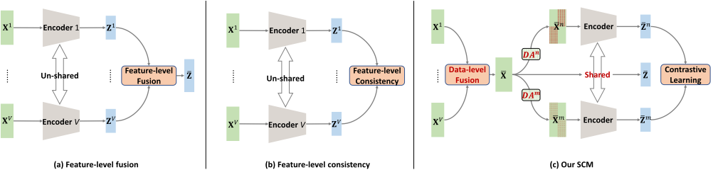
To address the aforementioned issues, we propose a novel framework entitled SCM: Simple Contrastive Multi-view clustering with data-level fusion as shown in Figure 1(c). Firstly, to avoid using multiple encoder networks as in previous methods, we propose shifting the fusion step from the feature-level to the data-level. In order to ensure that the fused data retains the information within multi-view data, we employ normalization and concatenation operations to achieve the data-level fusion without other operations. In this way, the discriminative information of different views can be encapsulated within different dimensions of the fused data, allowing us to search for data partitions in the fused data space, and thus handle multi-view learning problems as conveniently as single-view learning with a shared encoder network. Secondly, to enhance the robustness of deep model towards data noise and unavailability in real-world multi-view scenarios, we propose noise multi-view data augmentation and missing multi-view data augmentation to process the fused data. Furthermore, we employ instance-discriminative contrastive learning on the two types of augmented data, ensuring that the learned features are conducive to explore cross-view discriminative information while filtering the effect of noisy and unavailable data. Thirdly, we leverage the foundational SCM framework to conduct feature clustering and end-to-end clustering with known and unknown class number. Our main contributions are listed as follows:
- We propose a novel deep multi-view clustering framework (SCM) by data-level fusion for processing multiview data, which addresses the challenges of network customization and redundancy in previous methods.
- We develop two multi-view data augmentation techniques that specifically consider data noise and unavailability, marking contrastive learning with a shared encoder can effectively learn useful information from data.
- We implement several variants of our SCM framework equipped with simple network structure. Extensive experiments indicate that our method achieves comparable or superior clustering performance relative to state-of-
the-art methods. The simplicity of SCM is advantageous for its extension to other multi-view learning domains.
Notation definition In this paper, we represent matrices with uppercase bold letters and vectors with lowercase bold letters. Given a multi-view dataset {Xv ∈ RN×dv }Vv=1 , N and V respectively denote the sample size and the view number, and dv is the sample dimensionality of the v-th view data Xv .
2 Method
In this paper, we propose our SCM framework as shown in Figure 1(c), which not only can avoid the model customization for different views (this issue will exist in previous deep MVC methods as Figure 1(a-b)) by our data-level fusion with a shared network, but also can learn robust features by our multi-view data augmentation with contrastive learning.
2.1 Data-Level Fusion and Data Augmentation
To begin with, we introduce the basics in SCM framework, i.e., data-level fusion and multi-view data augmentation.
Data-level fusion Unlike previous methods that perform fusion operations at the feature-level, we advocate for data-level fusion of multi-view data to synergistically utilize the discriminative information of multiple views. The fused data will establish a bridge to mitigate the gap between multi-view learning and single-view learning, and avoid the redundancy and customization issues of multi-view encoder networks.
Specifically, we express the data-level fusion as a function:
where N(·) denotes the min-max normalization that brings the variables of different views into a uniform scale without distorting the ranges of values, [·] is the concatenation operation, and ¯X ∈ RN×D (D = ∑v dv) is defined as the fused data for all views. In this way, the discriminative information of different views can be encapsulated within different dimensions of the fused data. Traditional feature-level fusion after dimensionality reduction with different encoders might result in the loss of information due to data processing inequality.
Hence, in our data-level fusion, we refrain from employing complex mappings to ensure that the fused data retains the discriminative information from all views' raw data.
Multi-view data augmentation Motivated by the beneficial effects of data augmentation [Shorten and Khoshgoftaar, 2019] in computer vision, we propose multi-view data augmentation techniques targeted for the fused data to increase model representation ability, which simulates the scenarios of noisy and unavailable data in practical multi-view learning.
Specifically, considering the presence of noisy data within multi-view datasets, we design the noise multi-view data augmentation by adding noise on some views for each sample:
To be specific, we denote the v-th view data in the fused data as ¯Xv = N(Xv ) ∈ RN×dv . Then, for the i-th data ¯xvi ∈ ¯Xv , its noise-augmented data ¯nvi ∈ ¯Nv is generated by
where δv i is randomly sampled from an uniform distribution, and ϵ ∈ Rdv is random noise sampling from a Gaussian distribution N(0, σ2 ). p is a threshold that controls the proportion of noise-augmented data within multi-view data.
Further, given the case of data unavailability in multi-view datasets, we also design the missing multi-view data augmentation by masking values on some views for each sample:
To be specific, we denote the v-th view data in the fused data as ¯Xv = N(Xv ) ∈ RN×dv . Then, for the i-th data ¯xvi ∈ ¯Xv , its missing-augmented data ¯mvi ∈ ¯Mv is generated by
where A ∈ {0, 1}N×V is a random indicator matrix, which ensures that for the i-th sample, data from different views can be zeroed out to simulate the state of data unavailability while guaranteeing that at least one view remains available. We have ∑i (I{∑v aiv < V })/N = r where I{·} denotes the indicator function, and r is a threshold that controls the proportion of missing-augmented data within multi-view data.
The augmented data ¯Xn and ¯Xm are dynamically generated during training and thus will make SCM can be robust to the data noise and unavailability by the interaction among multiple views. Moreover, ¯Xn , ¯Xm ∈ RN×D are the same in data format and can be trained with a shared deep model.
2.2 Contrastive Clustering in SCMFramework
Given the fused data and its augmented data, we present our SCM equipped with contrastive leaning, as well as its variants with reconstruction regularization and end-to-end clustering. Contrastive learning For the augmented data ¯Xn and ¯Xm, we utilize a shared encoder Eθ (parameterized by θ) to extract their features ¯Zn ∈ RN×Z and ¯Zm ∈ RN×Z , respectively:
We then apply instance-discriminative contrastive learning on ¯Zn and ¯Zm, to explore discriminative information across multiple views within the fused data. Specifically, for a minibatch samples B, {¯zni ∈ ¯Zn , ¯zmi ∈ ¯Zm}i=1,...,|B| are |B| positive pairs. For each ¯zni , its (2|B| - 2) negative pairs is {¯zni , ¯zvj }v=n,m j̸=i and {¯zvj }v=n,m j̸=i is denoted as a set of s-. The InfoNCE [Oord et al., 2018] loss for a single positive pair with multiple negative pairs is given by:
where τ denotes a temperature parameter and the distance between two sample features (e.g., ¯zni ∈ ¯Zn and ¯zmj ∈ ¯Zm) is measured by cosine similarity:
The overall InfoNCE loss for the batch is defined as follows:
In this SCM framework, contrastive learning encourages the encoder to map positive pairs closer together relative to negative pairs in the feature space, thus learning to discriminate different samples of the fused data. Specially, the feature ¯Zn can learn from noiseless views in data ¯Xm, and the feature ¯Zm can learn from available views in data ¯Xn , so we achieve the interaction of multi-view information in a shared model and aim to increase the model robustness. Then, we design model regularization and end-to-end prediction for clustering. Reconstruction regularization Since clustering is an unsupervised learning task, using a decoder network to reconstruct the original data from learned features can naturally create a self-supervised signal, that encourages the capture of discriminative structures hidden within the data. This reconstruction regularization has been successfully applied to many deep MVC methods [Trosten et al., 2023], which typically use unshared decoder networks for reconstructing different views. Within the context of our proposed multi-view data augmentation, we introduce a novel approach by employing a shared decoder network for achieving reconstruction regularization.
Specifically, we leverage a shared decoder network Dϕ (parameterized by ϕ) and establish three different reconstruction losses for the fused data and augmented data as follows:
where ¯Hn , ¯Hm, ¯H are the hidden features between data ¯Xn , ¯Xm, ¯X and features ¯Zn , ¯Zm, ¯Z, respectively. θ′ denotes partial network parameters within θ. For example, we have ¯Hn = Eθ′ ( ¯Xn ) and ¯Zn = Eθ( ¯Xn ) = Eθ\θ′ ( ¯Hn ). It is noteworthy that we impose the reconstruction loss on ¯Hn , ¯Hm, ¯H to avoid the inductive conflicts with the contrastive loss applied on ¯Zn , ¯Zm [Xu et al., 2022]. Then, the overall reconstruction loss is formulated as follows:
This overall reconstruction loss could be viewed as a combination of different reconstruction regularization [Xu et al., 2023]. Concretely, LnRE encourages the hidden feature ¯Hn to reconstruct the noiseless data ¯X from noise-augmented data ¯Xn . LmRE enables the hidden feature ¯Hm to reconstruct the available data ¯X from missing-augmented data ¯Xm. L-RE regularizes the hidden feature ¯H obtained by the noiseless and available data ¯X, for usage in subsequent clustering tasks. End-to-end clustering Existing deep MVC methods for achieving end-to-end clustering primarily employ two strategies: I) In feature-level fusion methods, they often obtain cluster pseudo-labels on the fused features and then train a cluster network through self-training; II) For feature-level consistency methods, they usually set up separate cluster networks for different views and achieve consistent clustering through contrastive learning. It is worth noting that existing methods tend to require pre-setting the number of clusters K to design the dimensionality of the model's cluster network for each dataset, and our experiments in Section 3.2 find that fixed K is harmful for clustering performance. To make our model architecture compatible with different Ks of datasets, we propose end-to-end clustering on the basis of our SCM.
Specifically, we add a H-dimensional cluster network behind the feature ¯Z and obtain clustering labels ¯Q ∈ RN×H :
where Rω is a linear MLP network that organizes the dimensionality of clustering prediction to H. To extract known clustering structure information from ¯Z, we utilize a clustering method that does not depend on class number, such as Density Peaks [Rodriguez and Laio, 2014], which automatically searches the feature space to obtain a set of anchor points A = {aj}|A| j=1 , aj ∈ RZ . Further, through nearest neighbor assignment, we obtain the clustering labels ¯P ∈ {0, 1}N×H (pij ∈ ¯P) for N samples as follows:
Actually, we have ¯P = [{0, 1}N×|A| ; {0}N×(H-|A|) ]. As a result, the first |A| dimensions of the matrix ¯P contain the cluster information in the learned features, and the last (H - |A|) dimensions are all zeros. To achieve end-to-end clustering, we minimize the following mean squared error:
In implementation, the dimensionality number H can be set much larger than the potential class number of dataset, thus decoupling the design of the model's neural network structure from specific dataset. The final clustering prediction can still be obtained as follows, e.g., for the i-th sample:
Input: Multi-view dataset {X1 , X2 , . . . , XV } Setting: SCM(λ1, λ2 = 0), SCMRE(λ1 = 1, λ2 = 0), SCMEC(λ1 = 0, λ2 = 1), SCMEC+RE(λ1, λ2 = 1), rates of data augmentation p, r, std σ, batch size |B|, network parameters θ, ϕ, ω, learning rate η Data-level fusion ¯X= F(X1 ,X2 , . . . ,XV ) while not converging do Sampling mini-batch data ¯XB from ¯X ¯XnB = f nDA( ¯XB; p, σ), ¯XmB = f m DA( ¯XB; r) Compute ¯HnB , ¯HmB , ¯HB, ¯ZnB , ¯ZmB if λ1 == 0 then Compute L = LCO Update θ ← θ - η∇L(θ) else Compute L = LCO + LRE Update θ, ϕ ← θ, ϕ - η∇L(θ, ϕ) if λ2 == 1 then Compute ¯Z on ¯X and infer ¯P on ¯Z while not converging do Sampling mini-batch data ¯XB from ¯X ¯XnB = f nDA( ¯XB; p, σ), ¯XmB = f m DA( ¯XB; r) Compute ¯HnB , ¯HmB , ¯HB, ¯ZnB , ¯ZmB , ¯QB if λ1 == 0 then Compute L = LCO + LEC Update θ, ω ← θ, ω - η∇L(θ, ω) else Compute L = LCO + LRE + LEC Update θ, ϕ, ω ← θ, ϕ, ω - η∇L(θ, ϕ, ω) Output: ¯Z for SCM/SCMRE, ¯Q for SCMEC/EC+REFinally, we summarize the loss function in our method as
We leverage λ1, λ2 ∈ {0, 1} to obtain different variants of SCM framework: SCM(λ1, λ2 = 0), SCMRE(λ1 = 1, λ2 = 0), SCMEC(λ1 = 0, λ2 = 1), SCMEC+RE(λ1, λ2 = 1), whose training steps are shown in Algorithm 1.
Complexity analysis We let E denote the total training epochs, V and N are the number of views and the sample size of a dataset, |B| is the batch size in the mini-batch optimization. For each batch, the computational complexity of multi-view data augmentation is 2O(|B|), that of contrastive loss, reconstruction loss, and end-to-end clustering loss are O(|B|2 ), 3O(|B|), and O(|B|), respectively. The computational complexity to obtain clustering labels is O(N). For E training epochs, the computational complexity approximates to O(N) + (EN/|B|)O(|B|2 ) which is linear to sample size N. In terms of the memory consumption of deep model, the complexity in our SCM is 1/V of that in previous deep MVC methods, as the deep model in SCM is a shared network while that of other methods need V individual networks.
| BDGP | DIGIT | Fashion | NGs | VOC | WebKB | DHA | COIL-20 | Avg. | |
|---|---|---|---|---|---|---|---|---|---|
| ACC (mean±std%) | |||||||||
| K-Means | 44.3±2.9 | 78.1±2.3 | 71.2±1.3 | 20.6±0.2 | 48.7±0.8 | 61.7±0.8 | 65.6±2.9 | 42.1±3.0 | 54.0 |
| CPSPAN | 69.0±8.7 | 79.2±0.1 | 74.1±5.1 | 35.2±0.2 | 45.2±2.2 | 77.1±2.1 | 66.3±3.3 | 81.3±2.8 | 65.9 |
| CVCL | 90.7±7.8 | 99.5±0.1 | 99.0±0.1 | 56.8±7.7 | 31.5±4.1 | 74.1±3.0 | 66.2±6.3 | 100.0±0.0 | 77.2 |
| DSIMVC | 98.3±0.3 | 98.8±0.5 | 83.5±3.2 | 63.0±6.2 | 21.2±1.7 | 70.2±1.4 | 63.5±4.6 | 78.0±4.2 | 72.1 |
| DSMVC | 52.3±7.9 | 82.7±3.4 | 75.3±6.2 | 35.2±2.7 | 63.3±3.4 | 66.3±1.8 | 76.2±1.3 | 81.6±3.8 | 66.6 |
| MFLVC | 98.3±1.2 | 99.6±0.0 | 99.3±0.0 | 90.8±0.0 | 29.2±0.4 | 67.2±2.1 | 71.6±1.1 | 100.0±0.0 | 82.0 |
| SCM [ours] | 96.2±0.3 | 98.9±0.1 | 98.0±0.2 | 96.8±0.4 | 60.7±4.6 | 68.9±1.7 | 81.4±2.1 | 100.0±0.0 | 87.6 |
| SCMRE [ours] | 97.1±0.4 | 98.8±0.1 | 98.0±0.1 | 96.5±0.1 | 62.9±0.1 | 72.5±2.4 | 80.4±0.1 | 100.0±0.0 | 88.3 |
| NMI (mean±std%) | |||||||||
| K-Means | 57.3±4.1 | 72.2±1.1 | 66.8±1.2 | 1.9±0.3 | 36.0±2.0 | 0.2±0.1 | 79.8±0.1 | 63.3±1.0 | 47.2 |
| CPSPAN | 63.6±7.7 | 78.6±2.0 | 76.9±2.2 | 21.5±1.5 | 48.8±1.7 | 16.6±4.2 | 77.5±1.0 | 88.7±1.4 | 59.0 |
| CVCL | 78.5±0.9 | 98.5±0.2 | 97.5±0.1 | 31.7±7.8 | 31.7±2.6 | 24.6±2.6 | 75.4±3.3 | 100.0±0.0 | 66.6 |
| DSIMVC | 94.4±0.7 | 96.8±0.8 | 82.3±1.8 | 50.2±5.9 | 20.4±1.1 | 25.0±1.3 | 77.8±4.3 | 90.7±1.7 | 67.2 |
| DSMVC | 39.6±1.0 | 81.0±3.0 | 70.8±4.3 | 8.2±1.3 | 72.3±4.1 | 13.4±1.2 | 83.6±0.8 | 89.1±2.3 | 57.3 |
| MFLVC | 95.1±0.5 | 98.7±0.0 | 98.3±0.0 | 80.2±0.0 | 28.0±0.1 | 24.5±1.4 | 81.2±0.4 | 100.0±0.0 | 75.8 |
| SCM [ours] | 88.5±2.7 | 96.8±1.1 | 95.8±0.3 | 90.0±1.2 | 62.2±4.3 | 9.4±2.1 | 84.0±4.1 | 100.0±0.0 | 78.3 |
| SCMRE [ours] | 91.3±0.2 | 96.6±0.1 | 95.7±0.0 | 89.3±0.1 | 62.9±1.1 | 26.8±5.2 | 84.0±0.1 | 100.0±0.0 | 80.8 |
| ARI (mean±std%) | |||||||||
| K-Means | 25.7±5.8 | 63.1±1.9 | 57.4±1.0 | 21.0±0.0 | 12.4±3.4 | 1.4±0.0 | 59.7±2.7 | 39.7±2.1 | 35.1 |
| CPSPAN | 51.1±12.4 | 70.7±2.3 | 65.1±4.3 | 9.2±0.5 | 28.5±1.4 | 12.5±2.1 | 62.7±1.5 | 77.9±1.5 | 47.2 |
| CVCL | 73.4±12.3 | 98.8±0.2 | 97.7±0.2 | 28.1±10.7 | 18.9±3.3 | 19.8±3.3 | 53.6±6.3 | 100.0±0.0 | 61.3 |
| DSIMVC | 95.7±0.6 | 97.3±1.0 | 74.6±3.7 | 43.9±6.3 | 10.0±2.2 | 16.2±2.3 | 55.6±4.7 | 74.4±4.0 | 58.5 |
| DSMVC | 26.5±7.4 | 68.6±3.7 | 61.5±6.6 | 5.8±1.2 | 56.5±3.9 | 10.6±1.0 | 60.8±1.1 | 78.8±3.7 | 46.1 |
| MFLVC | 95.9±0.8 | 99.1±0.0 | 98.6±0.0 | 79.2±0.0 | 15.8±3.9 | 4.5±2.1 | 62.5±0.7 | 100.0±0.0 | 69.4 |
| SCM [ours] | 90.7±1.7 | 97.5±0.4 | 95.6±0.7 | 92.1±4.7 | 52.6±0.9 | 4.7±1.0 | 70.3±0.2 | 100.0±0.0 | 75.4 |
| SCMRE [ours] | 93.0±1.0 | 97.3±0.2 | 95.6±0.1 | 91.4±0.2 | 54.5±0.1 | 15.5±4.3 | 70.0±1.1 | 100.0±0.0 | 77.2 |
3 Experiment
3.1 Experimental Setup
Datasets We conduct experiments on 8 public datasets, including BDGP [Cai et al., 2012], DIGIT [Peng et al., 2019], Fashion [Xiao et al., 2017], NGs [Hussain et al., 2010], VOC [Everingham et al., 2010], WebKB [Sun et al., 2007], DHA [Lin et al., 2012], and COIL-20 [Nene et al., 1996]. Baselines The comparison methods include K-Means [MacQueen, 1967], Density peak clustering [Rodriguez and Laio, 2014], and deep MVC methods CPSPAN [Jin et al., 2023], CVCL [Chen et al., 2023], DSIMVC [Tang and Liu, 2022a], DSMVC [Tang and Liu, 2022b], MFLVC [Xu et al., 2022]. Implementation details To facilitate a fair comparison, we employed the same network architecture in [Xu et al., 2022; Tang and Liu, 2022a] to implement SCM. It is important to note that whereas previous methods necessitated multiple encoder-decoder networks, our SCM framework requires only one. Specifically, the encoder network structure can be depicted as a fully connected (Fc) MLP [Rosenblatt and others, 1962] with the configuration of ¯X- Fc500 - Fc500 - Fc2000 - ¯H- ¯Z- ¯Q, and the decoder network structure is ¯H - Fc2000 - Fc500 - Fc500 - ¯X. The activation function for the cluster network ¯Q is Softmax, while ReLU [Nair and Hinton, 2010] is used for all other activation functions. For all datasets used in our experiments, the dimensions of ¯H, ¯Z, and ¯Q were set to 256, 128, and 64, respectively. The optimizer was Adam [Kingma and Ba, 2014] with a learning rate of 0.0003, and the batch size was set to 256. Both the noise and missing rates of multi-view data augmentation were set to 0.25, and the noise variance was 0.4. Our SCM is implemented by PyTorch and its code is available in https://github.com/SubmissionsIn/SCM.
3.2 Result Analysis
Tables 1 and 2 showcase the clustering results of all comparison methods with known and unknown class number, respectively, where mean values of 5 runs are reported. Evaluation metrics include clustering ACC, NMI, and ARI.
Clustering with known class number When the class number is known, we report clustering results of comparison methods as shown in Table 1. Obviously, our methods, including vanilla SCM and reconstruction regularized SCMRE, achieve superior clustering performance. Specifically, the average results across 8 datasets indicate that our SCM achieved the improvement of 5% in ACC and 2% in NMI compared to the currently best-performing methods, while SCMRE achieved the improvement of 6% in ACC and 5% in NMI. In addition to superior clustering performance, our proposed data-level fusion makes SCM have simple contrastive multiview learning paradigm, which can avoid the issues of model redundancy and network customization in previous methods. Clustering with unknown class number To further explore the impact of the unknown class number, we report end-toend clustering results of different methods in Table 2. If the class number in models is fixed, previous end-to-end deep MVC methods often yield degraded results. This is because end-to-end clustering methods typically depend on the truth class number of datasets to design their model structures. In contrast, our methods (SCMEC and SCMEC+RE) still achieve best performance, for instance, the ACC of SCMEC and SCMEC+RE have 9% and 13% improvements to the best comparison methods, respectively. The reason is that our SCM has the decoupled design between the model structure and the setting of class number, which transfers the problem of sensitive class number from the model structure to the density peak algorithm and is beneficial for its applicability.
| BDGP | DIGIT | Fashion | NGs | VOC | WebKB | DHA | COIL-20 | Avg. | |
|---|---|---|---|---|---|---|---|---|---|
| ACC (mean±std%) | |||||||||
| Density Peaks | 21.8±0.0 | 18.3±0.0 | 20.0±0.0 | 21.0±0.0 | 9.2±0.0 | 61.4±0.0 | 13.8±0.0 | 39.4±0.0 | 25.6 |
| CPSPANF CN | 20.3±2.4 | 21.9±0.7 | 28.9±1.8 | 34.1±2.2 | 44.2±1.9 | 27.6±1.7 | 46.3±1.9 | 54.1±1.0 | 34.7 |
| CVCLF CN | 29.8±2.0 | 44.5±2.5 | 40.9±5.1 | 19.8±3.2 | 25.2±2.6 | 11.0±2.0 | 40.0±2.2 | 75.8±5.0 | 35.9 |
| DSIMVCF CN | 27.0±2.8 | 46.0±2.0 | 42.5±4.1 | 19.8±5.6 | 19.5±1.6 | 24.3±5.6 | 37.5±2.6 | 78.2±3.6 | 36.9 |
| DSMVCF CN | 19.2±1.0 | 28.6±1.6 | 28.2±1.2 | 11.3±0.6 | 44.1±2.0 | 8.2±0.4 | 62.1±1.9 | 68.0±1.3 | 33.7 |
| MFLVCF CN | 65.2±1.5 | 90.0±2.2 | 95.4±0.3 | 20.5±1.2 | 28.8±0.8 | 29.3±2.3 | 65.7±1.9 | 99.0±0.6 | 61.7 |
| SCMEC [ours] | 80.3±2.1 | 96.5±0.2 | 67.2±1.3 | 33.5±4.3 | 71.7±1.7 | 48.9±4.3 | 76.2±1.2 | 94.1±1.3 | 71.0 |
| SCMEC+RE [ours] | 79.8±8.4 | 97.0±1.8 | 85.3±0.3 | 37.3±1.4 | 72.6±7.6 | 54.6±2.4 | 75.7±4.2 | 94.6±3.1 | 74.6 |
| NMI (mean±std%) | |||||||||
| Density Peaks CPSPANF CN CVCLF CN DSIMVCF CN DSMVCF CN | 6.3±0.0 | 36.9±0.0 | 40.2±0.0 | 21.6±0.0 | 49.9±0.0 | 8.8±0.0 | 69.1±0.0 | 68.5±0.0 | 37.7 |
| 55.1±2.2 | 66.3±0.5 | 62.0±0.3 | 34.9±1.4 | 49.0±1.9 | 20.0±1.2 | 75.2±1.1 | 79.6±1.7 | 55.3 | |
| 53.4±2.8 | 67.5±2.0 | 63.2±3.5 | 32.3±2.8 | 27.0±2.0 | 19.7±0.5 | 64.4±2.5 | 87.3±2.5 | 51.8 | |
| 58.1±0.8 | 73.8±0.5 | 62.9±0.8 | 37.7±2.1 | 20.6±0.8 | 20.2±0.5 | 61.9±1.3 | 89.4±4.2 | 53.1 | |
| 50.4±0.6 | 64.3±1.0 | 57.2±0.5 | 20.3±1.0 | 64.5±1.5 | 8.2±0.8 | 76.8±0.5 | 83.5±0.5 | 53.1 | |
| MFLVCF CN | 78.3±0.7 | 84.2±2.2 | 96.0±0.1 | 44.2±0.3 | 27.5±0.2 | 21.4±0.4 | 75.4±1.0 | 99.6±0.2 | 65.8 |
| SCMEC [ours] | 69.5±2.0 | 94.6±0.4 | 68.9±0.3 | 10.5±4.2 | 66.8±2.0 | 11.2±5.2 | 83.7±4.2 | 96.5±0.1 | 62.7 |
| SCMEC+RE [ours] | 72.3±0.7 | 95.6±0.5 | 84.8±0.1 | 11.9±2.6 | 66.8±1.1 | 17.8±1.7 | 83.4±4.6 | 96.6±3.6 | 66.2 |
| ARI (mean±std%) | |||||||||
| Density Peaks CPSPANF CN CVCLF CN DSIMVCF CN | 0.2±0.0 | 12.2±0.0 | 17.4±0.0 | 1.1±0.0 | 2.5±0.0 | 3.9±0.0 | 7.0±0.0 | 36.0±0.0 | 10.0 |
| 16.6±1.2 | 25.0±0.6 | 30.5±2.4 | 11.0±2.0 | 30.8±3.3 | 7.5±1.0 | 40.9±1.5 | 62.1±0.4 | 28.1 | |
| 24.2±3.0 | 41.9±3.6 | 37.7±5.7 | 9.2±2.5 | 14.4±4.0 | 2.6±0.3 | 28.6±2.8 | 73.9±5.7 | 29.1 | |
| 23.3±1.6 | 45.8±2.5 | 38.6±4.9 | 13.2±4.2 | 9.2±1.2 | 5.7±1.7 | 28.2±1.8 | 77.7±2.9 | 30.2 | |
| DSMVCF CN | 14.7±0.5 | 28.3±0.9 | 26.4±0.3 | 2.8±1.3 | 34.2±0.1 | 1.1±0.1 | 52.4±1.4 | 71.3±0.5 | 28.9 |
| MFLVCF CN | 66.2±1.2 | 90.0±1.4 | 94.9±0.2 | 16.0±0.5 | 15.8±0.6 | 7.8±0.9 | 58.6±2.0 | 99.2±0.4 | 56.1 |
| SCMEC [ours] | 65.2±2.4 | 94.0±0.3 | 60.8±1.2 | 7.1±4.2 | 61.5±3.1 | 3.0±4.3 | 67.8±0.4 | 93.3±2.2 | 56.6 |
| SCMEC+RE [ours] | 67.8±11.8 | 95.7±1.3 | 79.2±0.2 | 8.6±1.6 | 63.3±1.0 | 15.0±4.2 | 66.7±4.6 | 93.1±3.6 | 61.2 |
| BDGP | DIGIT | Fashion | NGs | VOC | WebKB | DHA | COIL-20 | Avg. | |
|---|---|---|---|---|---|---|---|---|---|
| ACC | |||||||||
| SCMw/o DA SCMw/ f m DA SCMw/ f nDA SCM | 42.3 63.7 59.5 96.2 | 49.1 98.7 57.1 98.9 | 16.5 86.9 24.0 98.0 | 34.2 42.3 59.8 96.8 7.7 | 56.4 57.1 62.5 60.7 NMI | 52.7 67.6 58.7 68.9 | 56.9 82.0 74.0 81.4 | 45.2 100.0 54.6 100.0 | 44.2 74.8 56.3 87.6 |
| SCMw/o DA SCMw/ f m DA SCMw/ f nDA SCM | 24.7 52.9 51.1 | 45.2 96.5 59.6 96.8 | 4.1 88.7 15.7 | 14.4 39.8 90.0 | 54.8 54.2 63.6 62.2 ARI | 0.2 21.1 1.8 9.4 | 66.5 85.2 77.9 | 57.4 100.0 67.1 100.0 | 32.6 64.1 47.1 |
| 88.5 | 95.8 | 84.0 | |||||||
| 1.8 81.0 | 41.6 42.9 54.7 | -0.4 | 71.7 59.4 | ||||||
| 16.2 | 29.0 97.2 | 5.3 | 0.1 12.5 | 39.0 | 31.2 | 78.3 20.5 | |||
| SCMw/o DA SCMw/ f m DA SCMw/ f nDA | 40.9 35.7 | 39.7 | 5.9 | 11.5 32.2 | 100.0 43.0 | 57.2 33.8 | |||
| SCM | 90.7 | 97.5 | 95.6 | 92.1 | 52.6 | 4.7 | 100.0 | ||
| 70.3 | 75.4 | ||||||||
| BDGP | DIGIT | Fashion | NGs | VOC | WebKB | DHA | COIL-20 | Avg. | |
|---|---|---|---|---|---|---|---|---|---|
| ACC | |||||||||
| SCMRE | 97.1 | 98.8 | 98.0 | 96.5 | 62.9 | 72.5 | 80.4 | 100.0 | 88.3 |
| SCMRE w/o LRE | 96.2 | 98.9 | 98.0 | 96.8 | 60.7 | 68.9 | 81.4 | 100.0 | 87.6 |
| SCMRE w/o LCO | 93.7 | 80.2 | 77.3 | 68.6 | 47.6 | 51.0 | 75.0 | 65.1 | 69.8 |
| SCMEC+RE | 79.8 | 97.0 | 85.3 | 37.3 | 72.6 | 54.6 | 75.7 | 94.6 | 74.6 |
| SCMEC+RE w/o LEC | 36.8 | 39.5 | 24.8 | 17.6 | 35.3 | 17.1 | 39.1 | 51.4 | 32.7 |
| NMI | |||||||||
| SCMRE | 91.3 | 96.6 | 95.7 | 89.3 | 62.9 | 26.8 | 84.0 | 100.0 | 80.8 |
| SCMRE w/o LRE | 88.5 | 96.8 | 95.8 | 90.0 | 62.2 | 9.4 | 84.0 | 100.0 | 78.3 |
| SCMRE w/o LCO | 84.3 | 73.2 | 75.6 | 53.8 | 53.4 | 5.9 | 80.3 | 81.0 | 63.4 |
| SCMEC+RE | 72.3 | 95.6 | 84.8 | 11.9 | 66.8 | 17.8 | 83.4 | 96.6 | 66.2 |
| SCMEC+RE w/o LEC | 44.0 | 42.5 | 28.6 | 16.8 | 39.3 | 12.0 | 56.3 | 62.8 | 37.8 |
| ARI | |||||||||
| SCMRE | 93.0 | 97.3 | 95.6 | 91.4 | 54.5 | 15.5 | 70.0 | 100.0 | 77.2 |
| SCMRE w/o LRE | 90.7 | 97.5 | 95.6 | 92.1 | 52.6 | 4.7 | 70.3 | 100.0 | 75.4 |
| SCMRE w/o LCO | 85.0 | 66.7 | 67.5 | 47.4 | 38.3 | -4.5 | 60.7 | 65.2 | 53.3 |
| SCMEC+RE | 67.8 | 95.7 | 79.2 | 8.6 | 63.3 | 15 | 66.7 | 93.1 | 61.2 |
| SCMEC+RE w/o LEC | 25.7 | 24.8 | 11.5 | 4.6 | 18.0 | 18.0 | 26.1 | 37.3 | 20.7 |
3.3 Ablation Study
In this part, we first investigate the key contributions in our proposed noise and missing multi-view data augmentation, and then analyze the different components in loss function.
Multi-view data augmentation As shown in Table 3, firstly, SCM w/o DA is a variant without any data augmentation, which achieves unsatisfactory clustering performance. Furthermore, SCM w/ f nDA and SCM w/ f m DA are variants that incorporate the noise multi-view data augmentation and the missing multi-view data augmentation defined in this paper, respectively, and they both show significant improvements over SCM w/o DA. Finally, SCM combines two types of data augmentation and achieves further substantial improvements, confirming the importance of our specially designed noise and missing multi-view data augmentation.

Loss components In Table 4, we conduct ablation studies on three losses using SCMRE and SCMEC+RE as baselines. Compared to SCMRE, removing the reconstruction regularization loss in variant SCMRE w/o LRE results in a slight performance decline, while removing the contrastive loss in variant SCMRE w/o LCO leads to a severe performance decrease. Furthermore, compared to the end-to-end clustering setting of SCMEC+RE, removing the end-to-end clustering loss in variant SCMEC+RE w/o LEC also significantly degrades model performance. These results indicate that LCO plays the most crucial role in contrastive multi-view clustering, and LEC is vital for end-to-end clustering, with LRE serving a supporting role to regularize the feature learning.
3.4 Model Analysis
In this part, we conduct visualization analysis on the parameters and the training process in our SCM framework.
Data augmentation rates {p, r} In SCM framework, we tune the noise multi-view data augmentation rate p and the missing multi-view data augmentation rate r within the range [0, 0.25, 0.5, 0.75, 1.0], with results depicted in Figure 2. We observe that moderately increasing p and r significantly benefits the model in learning precise clustering structures within multi-view datasets. The underlying mechanism is that our noise and missing multi-view data augmentation compel the model to focus on the interaction and complementarity across views, thereby making the feature learning more robust to inherent noise and unavailable samples in multi-view data. In comparison experiments, p and r were set to 0.25.
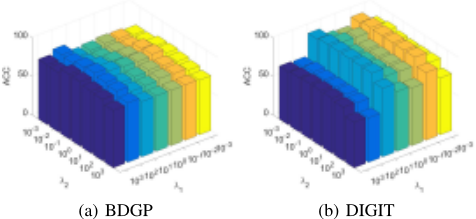
Trade-off parameters {λ1, λ2} In our method, trade-off parameters λ1, λ2 ∈ {0, 1} control the different settings in SCM framework. In Figure 3, we adopt the setting of SCMEC+RE and further explore the sensibility of λ1 and λ2 within the range of [10-3 , 10-2 , 10-1 , 100 , 101 , 102 , 103 ]. The optimal values of λ1 and λ2 are different across different datasets and this outcome is within expectations. Trade-off parameters generally have a minimal sensibility on the performance within the range of [10-1 , 101 ]. In all experiments, we did not specifically tune λ1 and λ2, and their values were fixed at 0 or 1 to implement different variants of SCM.
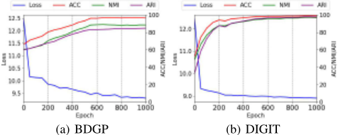
Training loss and performance In Figure 4, we record the loss and clustering accuracy curves during the training process of SCM. It is observed that the loss curve exhibits a smooth and consistent decline, indicating that SCM framework has well convergence. Concurrently, the steadily rising clustering accuracy suggests that the model is progressively learning the correct clustering structure of the dataset.
4 Conclusion
In this paper, we propose a novel contrastive multi-view clustering framework with data-level fusion, namely SCM. Specifically, our proposed data-level fusion effectively integrates multi-view information and avoids the issues of customization and redundancy of networks in previous methods. Moreover, we define two types of multi-view data augmentation approaches based on the data-level fusion, which enhances the robustness of model towards noisy and unavailable views in multi-view data. We apply the SCM framework to feature clustering and end-to-end clustering with known and unknown class number, and extensive experiments validate its effectiveness and superiority. Our SCM simplifies multiview contrastive learning with a shared deep network, and we hope it could bring fresh insights into multi-view learning.
Acknowledgments
This work was supported in part by the National Key Research & Development Program of China under Grant 2022YFA1004100, Medico-Engineering Cooperation Funds from University of Electronic Science and Technology of China under Grant ZYGX2022YGRH009 and Grant ZYGX2022YGRH014, Guangxi Natural Science Foundation (2023GXNSFBA026010), Research Fund of Guangxi Key Lab of Multi-source Information Mining & Security (22-A03-02), Innovation Project of Guangxi Graduate Education (XJCY2022009).
@inproceedings{ijcai2024p519,
  title     = {Simple Contrastive Multi-View Clustering with Data-Level Fusion},
  author    = {Luo, Caixuan and Xu, Jie and Ren, Yazhou and Ma, Junbo and Zhu, Xiaofeng},
  booktitle = {Proceedings of the Thirty-Third International Joint Conference on
               Artificial Intelligence, {IJCAI-24}},
  publisher = {International Joint Conferences on Artificial Intelligence Organization},
  editor    = {Kate Larson},
  pages     = {4697--4705},
  year      = {2024},
  month     = {8},
  note      = {Main Track},
  doi       = {10.24963/ijcai.2024/519},
  url       = {https://doi.org/10.24963/ijcai.2024/519},
}
TY - CPAPER TI - Simple Contrastive Multi-View Clustering with Data-Level Fusion AU - Luo, Caixuan AU - Xu, Jie AU - Ren, Yazhou AU - Ma, Junbo AU - Zhu, Xiaofeng T2 - Proceedings of the Thirty-Third International Joint Conference on Artificial Intelligence, IJCAI-24 PB - International Joint Conferences on Artificial Intelligence Organization PY - 2024 SP - 4697 EP - 4705 DO - 10.24963/ijcai.2024/519 UR - https://doi.org/10.24963/ijcai.2024/519 ER -Copied
Machine-readable versions of this paper, for tools and AI agents:





