
Estimating Conditional Average Treatment Effects via Sufficient Representation Learning
Proceedings of the Thirty-Third International Joint Conference on Artificial Intelligence. Main Track. Pages 4894-4901.
https://doi.org/10.24963/ijcai.2024/541
Keywords
- Machine Learning: ML: Causality
- Machine Learning: ML: Regression
- Machine Learning: ML: Supervised Learning
- Machine Learning: ML: Representation learning
Abstract
Estimating the conditional average treatment effects (CATE) is very important in causal inference and has a wide range of applications across many fields. In the estimation process of CATE, the unconfoundedness assumption is typically required to ensure the identifiability of the regression problems. When estimating CATE using high-dimensional data, there have been many variable selection methods and neural network approaches based on representation learning, while these methods do not provide a way to verify whether the subset of variables after dimensionality reduction or the learned representations still satisfy the unconfoundedness assumption during the estimation process, which can lead to ineffective estimates of the treatment effects. Additionally, these methods typically use data from only the treatment or control group when estimating the regression functions for each group. This paper proposes a novel neural network approach named CrossNet to learn a sufficient representation for the features, based on which we then estimate the CATE, where cross indicates that in estimating the regression functions, we used data from their own group as well as cross-utilized data from another group. Numerical simulations and empirical results demonstrate that our method outperforms the competitive approaches.
- [Athey and Imbens, 2016] Susan Athey and Guido Imbens. Recursive partitioning for heterogeneous causal effects. Proceedings of the National Academy of Sciences, 113(27):7353-7360, 2016.
- [Chauhan et al., 2023] Vinod K Chauhan, Soheila Molaei, Marzia Hoque Tania, Anshul Thakur, Tingting Zhu, and David A Clifton. Adversarial de-confounding in individu- alised treatment effects estimation. In International Con- ference on Artificial Intelligence and Statistics, pages 837- 849. PMLR, 2023.
- [Curth and van der Schaar, 2021] Alicia Curth and Mihaela van der Schaar. Nonparametric estimation of heteroge- neous treatment effects: From theory to learning algo- rithms. In International Conference on Artificial Intelli- gence and Statistics, pages 1810-1818. PMLR, 2021.
- [Green and Kern, 2012] Donald P Green and Holger L Kern. Modeling heterogeneous treatment effects in survey ex- periments with bayesian additive regression trees. Public opinion quarterly, 76(3):491-511, 2012.
- [Hansen and Bowers, 2009] Ben B Hansen and Jake Bow- ers. Attributing effects to a cluster-randomized get-out- the-vote campaign. Journal of the American Statistical Association, 104(487):873-885, 2009.
- [Hassanpour and Greiner, 2019a] Negar Hassanpour and Russell Greiner. Counterfactual regression with impor- tance sampling weights. In IJCAI, pages 5880-5887, 2019. IJCAI
- [Hassanpour and Greiner, 2019b] Negar Hassanpour and Russell Greiner. Learning disentangled representations for counterfactual regression. In International Conference on Learning Representations, 2019.
- [Hill, 2011] Jennifer L Hill. Bayesian nonparametric mod- eling for causal inference. Journal of Computational and Graphical Statistics, 20(1):217-240, 2011.
- [Kennedy, 2020] Edward H Kennedy. Towards optimal dou- bly robust estimation of heterogeneous causal effects. arXiv preprint arXiv:2004.14497, 2020.
- [Kulis et al., 2009] Brian Kulis, Mátyás A Sustik, and Inder- jit S Dhillon. Low-rank kernel learning with bregman ma- trix divergences. Journal of Machine Learning Research, 10(2), 2009.
- [Künzel et al., 2019] Sören R Künzel, Jasjeet S Sekhon, Pe- ter J Bickel, and Bin Yu. Metalearners for estimat- ing heterogeneous treatment effects using machine learn- ing. Proceedings of the national academy of sciences, 116(10):4156-4165, 2019.
- [LaLonde, 1986] Robert J LaLonde. Evaluating the econo- metric evaluations of training programs with experimen- tal data. The American economic review, pages 604-620, 1986.
- [Mooij et al., 2016] Joris M Mooij, Jonas Peters, Dominik Janzing, Jakob Zscheischler, and Bernhard Schölkopf. Distinguishing cause from effect using observational data: methods and benchmarks. The Journal of Machine Learn- ing Research, 17(1):1103-1204, 2016.
- [Robins and Rotnitzky, 1995] James M Robins and Andrea Rotnitzky. Semiparametric efficiency in multivariate re- gression models with missing data. Journal of the Ameri- can Statistical Association, 90(429):122-129, 1995.
- [Rolling and Yang, 2014] Craig A Rolling and Yuhong Yang. Model selection for estimating treatment effects. Journal of the Royal Statistical Society: Series B (Statisti- cal Methodology), 76(4):749-769, 2014.
- [Rosenbaum, 2007] Paul R Rosenbaum. Interference be- tween units in randomized experiments. Journal of the american statistical association, 102(477):191-200, 2007.
- [Rubin, 2005] Donald B Rubin. Causal inference using po- tential outcomes: Design, modeling, decisions. Journal of the American Statistical Association, 100(469):322-331, 2005.
- [Shalit et al., 2017] Uri Shalit, Fredrik D Johansson, and David Sontag. Estimating individual treatment effect: gen- eralization bounds and algorithms. In International con- ference on machine learning, pages 3076-3085. PMLR, 2017.
- [Shi et al., 2019] Claudia Shi, David Blei, and Victor Veitch. Adapting neural networks for the estimation of treatment effects. Advances in neural information processing sys- tems, 32, 2019.
- [Smith and Todd, 2005] Jeffrey A Smith and Petra E Todd. Does matching overcome lalonde's critique of nonexper- imental estimators? Journal of econometrics, 125(1- 2):305-353, 2005.
- [VanderWeele, 2019] Tyler J VanderWeele. Principles of confounder selection. European journal of epidemiology, 34:211-219, 2019.
- [Wager and Athey, 2018] Stefan Wager and Susan Athey. Estimation and inference of heterogeneous treatment ef- fects using random forests. Journal of the American Sta- tistical Association, 113(523):1228-1242, 2018.
- [Whitmore, 2005] Diane Whitmore. Resource and peer im- pacts on girls' academic achievement: Evidence from a randomized experiment. American Economic Review, 95(2):199-203, 2005.
- [Yao et al., 2021] Liuyi Yao, Zhixuan Chu, Sheng Li, Yaliang Li, Jing Gao, and Aidong Zhang. A survey on causal inference. ACM Transactions on Knowledge Dis- covery from Data (TKDD), 15(5):1-46, 2021.
- [Yu et al., 2021] Shujian Yu, Ammar Shaker, Francesco Ale- siani, and Jose Principe. Measuring the discrepancy be- tween conditional distributions: methods, properties and applications. In Proceedings of the Twenty-Ninth Interna- tional Conference on International Joint Conferences on Artificial Intelligence, pages 2777-2784, 2021. IJCAI
- [Zhang et al., 2021] Weijia Zhang, Lin Liu, and Jiuyong Li. Treatment effect estimation with disentangled latent fac- tors. In Proceedings of the AAAI Conference on Artificial Intelligence, volume 35, pages 10923-10930, 2021.
References were extracted automatically from the PDF and may contain errors.
Full text extracted automatically from the PDF; figures, tables and equations may differ. The PDF is the version of record.
1 Introduction
Estimating the CATE, also known as individual treatment effects (ITE) or heterogeneous treatment effects (HTE), is of great importance in causal inference and is widely applied in numerous fields [LaLonde, 1986; Athey and Imbens, 2016; Mooij et al., 2016; Yao et al., 2021]. In the medical field, the estimation of CATE can be applied to precision medicine, achieving personalized matching of treatment plans. In the socio-economic domain, the setting of policies and preassessment of their effects also rely on the estimation of treatment effects. In the field of advertising recommendations, making accurate recommendations of different ads to different groups can effectively save costs and enhance the effectiveness of the advertising. All these depend on the accurate estimation of CATE.
The estimation of the CATE is typically divided into randomized experimental studies [Whitmore, 2005; Rosenbaum, 2007] and observational data studies, with the distinction being whether the allocation of interventions is completely random. Due to the constraints of real-world settings and specific problems, we are often unable to conduct randomized experimental studies. For example, when analyzing the impact of smoking on lung cancer, we cannot ethically require some participants to smoke over an extended period. On the other hand, randomized experiments also come with high costs. Therefore, most researches are based on observational data, and this article is no exception. Most of the literature on research based on observational data operates under the assumption of unconfoundedness:
Assumption 1 (Unconfoundedness). Given the observed variables, the treatment variable is independent with the potential outcomes: Y (1), Y (0) ⊥ T | x.
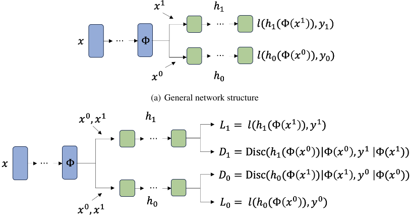
The meaning of this assumption is that the features we can collect contain all the information that could simultaneously affect both the treatment variable and the outcome variable, thereby creating a situation similar to a randomized experiment, where the allocation of interventions is completely random given these features. On the other hand, since we can only observe one of the two potential outcomes, we can not directly identify the CATE from the observational data unless the assumption of unconfoundedness holds. As we collect more data and the dimensionality of features increases, it becomes easier for the unconfoundedness assumption to be satisfied [Rolling and Yang, 2014]. However, when estimating CATE using high-dimensional data, many studies perform variable selection [VanderWeele, 2019] or representation learning [Shalit et al., 2017; Shi et al., 2019; Hassanpour and Greiner, 2019a; Hassanpour and Greiner, 2019b; Zhang et al., 2021; Chauhan et al., 2023] on the original data, and the resulting estimates of the treatment effect are based on the selected subset of variables or learned representations as shown in Figure 1 (a). These methods do not verify whether the representations or the selected subset of variables still meet the unconfoundedness assumption, nor do
(b) Our network structure
Figure 1: Φ is a learned representation. h1 and h0 are two hypothesis or predictive functions for y based on Φ in treated and control group respectively. l(·) is a loss function, where we use mean squared error loss. Disc(·) means the discrepancy. x1 , y1 and x0 , y0 are the covariates and responses corresponding to treated group sample and control group sample respectively.
they make additional assumptions, that is, we are unable to confirm whether Y (1), Y (0) ⊥ T | Φ(x) holds or not. If the unconfoundedness assumption no longer holds, the estimates of treatment effects based on Φ(x) are also no longer valid. Therefore, we propose a new type of neural network structure that, by imposing specific regularization terms, to ensure the learned representations still satisfy the unconfoundedness assumption, thus making the final treatment effect estimates accurate and valid.
On the other hand, most of the neural network approaches are conducted under the T-learner framework, which involves estimating a separate regression function for the treated group and the control group respectively, and then obtaining a plugin estimator by taking the difference between the two regression functions. However, as shown in Figure 1 (a), in training the regression functions for the treatment and control groups, they typically use data from their respective groups, that is, the treated group's hypothesis function is estimated using data from the treated group, and the control group's hypothesis function is estimated using data from the control group, which can lead to an underutilization of data. Actually, the goal is to estimate the treatment effect, not to achieve highly accurate estimates of the two hypothesis functions. Due to selection bias, having precise estimates for the two hypothesis functions does not always lead to an accurate estimate of the treatment effect. If we train the models using data from each group independently, we will lose the cross-information between groups. This results in the regression function of the treatment group not being well-suited for the data of the control group, and vice versa. [K¨unzel et al., 2019] proposed X-leaner, where they use data from another group to evaluate the hypothesis functions and then take average of the treatment effect under treated and control groups. However, they do not apply the data from another group into the training process in fact. The method we propose makes use of the full sample information when training the hypothesis functions. Through the design of the objective function, the treatment and control group data play different roles, aiming to achieve different optimization effects. The main contributions in this paper are as follows:
- We define a sufficient representation in causal inference, which not only has strong predictive power for potential outcomes, but also needs to satisfy the unconfoundedness assumption. We propose a novel objective function that enables us to learn the sufficient representations.
- During the training of the hypothesis functions, we use data from their own group as well as cross-utilize data from another group, allowing the two learned hypothesis functions to have good predictive capability for the counterfactual outcomes, thereby obtaining a more accurate estimate of the treatment effect.
- The regularization terms in our method take into account the information of the conditional distributions of counterfactual outcomes, which reduces the selection bias effectively and is more in line with the intuition of causal inference.
The rest of this paper is organized as follows. In Section 2, we discuss related works. Our proposed approach is represented in Section 3. In Section 4, we conduct Monte Carlo simulation and experiments. Finally, we give a conclusion in Section 5.
2 RelatedWork
[K¨unzel et al., 2019] proposed the concept of metalearners for estimating CATE, which decomposes the problem of estimating CATE into multiple sub-problems, each of which can be addressed using any supervised or regression machine learning method. [K¨unzel et al., 2019] was the first to combine metalearners with CATE, categorizing the previous methods into two types. The first type is S-Learner, where "S" denotes single. We can model the treatment variable together with other covariates using a single model, where only one estimator for µ(x, t) = E[Y |X = x, T = t] is obtained. Then, the estimate for CATE can be written as ˆ τS(x) = ˆµ(x, 1)-ˆµ(x, 0). Under this framework, [Hill, 2011], [Green and Kern, 2012] conducted research with Bayesian Additive Regression Trees (BARTs) as the baseline model. [Athey and Imbens, 2016] explored this further using tree-based models as the benchmark. The biggest shortcoming of the S-learner is that it does not take into account the interaction between covariates and the treatment variable, that is, it does not allow for the hypothesis functions of the treatment and control groups to have different forms.
The second type is T-learner, where "T" denotes two. We can model the treatment group and control group separately, obtaining estimates for two regression functions µ1(x) = E[Y (1)|X = x] and µ0(x) = E[Y (0)|X = x]. By further subtracting them, we can obtain the estimate ˆ τT (x) = ˆµ1(x) - ˆµ0(x) for CATE. Under this framework, [Hansen and Bowers, 2009] and [Wager and Athey, 2018] proposed causal forest, where they used random forest as the benchmark. In recent years, there have also been many methods based on representation learning and neural networks, which are also a type of T-learner. [Shalit et al., 2017] proposed the CFRNet, a neural network architecture that first learns a representation, and then by imposing a penalty on the integral probability metric measure of the representation between the treated and control groups, the model mitigates selection bias through a balanced representation learning. This work derived a bound for the expected error of the estimator for CATE given a fixed representation, where the hypothesis functions are defined over this representation. The key assumption is that this representation is a one-to-one function, so that the unconfoundedness assumption holds given this representation. This is a strong condition, as not all network architectures are invertible during the process of representation learning. [Shi et al., 2019] proposed Dragonnet based on the sufficiency of the propensity score for treatment effect estimation. The neural network architecture learns a shared representation, which is then used to model the two hypothesis functions and the propensity scores, ensuring that this representation simultaneously contains information that can predict both the outcomes and the treatment variable. [Hassanpour and Greiner, 2019b] proposed a context-aware importance sampling re-weighing scheme, built on top of a representation learning module. In [Shalit et al., 2017], the weight of the loss is simply based on the sample size, which is wi = 1/Pr(ti = 1). [Hassanpour and Greiner, 2019a] further eliminates selection bias by estimating the nominal distribution of the representation, followed by importance sampling re-weighting. They use 1 +Pr(ϕi | 1 - ti)/Pr(ϕi | ti) as the loss weight. Another category of neural network approaches estimates the CATE by learning a disentangled representation, or disentangled latent factors. [Zhang et al., 2021] proposed a data-driven algorithm TEDVAE to infer latent factors and disentangled them into three disjoint sets, which are to predict treatment, outcome, or both. [Hassanpour and Greiner, 2019b] also divided the information contained in all the covariates into three non-overlapping parts, characterizing them by learning three disentangled representations, and then modeled the treatment and outcome based on these representations. [Curth and van der Schaar, 2021], [Chauhan et al., 2023] further divided the features into five parts, corresponding to treatment t, treated group outcomes µ1, control group outcomes µ0, both µ1 and µ0, and all of treatment and outcomes.
[K¨unzel et al., 2019] proposed the third metaalgorithm: Xleaner, which first used the T-learner approach to estimate two hypothesis functions. Then, by cross-utilizing the data, they substituted data from the other group into the hypothesis function to predict the counterfactual outcomes. By comparing these predictions with the factual outcomes, we can obtained the estimates of the individual treatment effects for all samples, which is ˜D1 i = Y 1 i - ˆµ0(X1 i ), ˜D0 i = ˆµ1(X0 i ) - Y 0 i , where ˜D1 is the predicted ITE for treated group, and ˜D0 i is the predicted ITE for control group. Subsequently, by regressing these individual effects against the individuals' characteristics, we can obtain the estimates of the treatment effects under treated group (ITT) ˆ τ1(x) and control group (ITC) ˆ τ0(x). Finally, they take a weighted average of these two estimates, resulting in the estimate for CATE ˆ τX(x) = g(x) · ˆ τ1(x) + (1 - g(x)) · ˆ τ0(x). This method also cross-utilizes the data from different groups, but does not participate in the training process of their respective hypothesis functions, that is, the estimation of µ1(x) and µ0(x). In fact, when the unconfoundedness assumption is satisfied, ˆ τ0(x) and ˆ τ1(x) should be equal, which we will mention in the next section. [K¨unzel et al., 2019] averages ˆ τ0(x) and ˆ τ1(x) using weights, while our approach encourages equality between them through a regularization term. This allows the data from different groups to participate in the training process of each other's hypothesis functions, since the estimation for ˆ τ0(x) and ˆ τ1(x) requires data from both treated and control groups. Our method fully utilizes the information from all the data and ensures that the unconfoundedness assumption is met given the learned representation.
[Curth and van der Schaar, 2021] summarizes lots of nonparametric statistical methods and machine learning approaches, from theoretical research to experiment, and supplements the field of CATE with meta-learners. The author collectively refers to the aforementioned S-learner and T-learner as one-step methods. That is, they estimate the conditional expectation only once and then use a plug-in method to estimate the CATE. The author defines a two-step method, which first involves estimating the nuisance parameters η = (µ0(x), µ1(x), π(x)) to obtain ˆ η, then regressing the pseudoresponse variable ˜ Y ˆ eta , which depends on the nuisance parameters, on x. Here we consider the pseudo-response variable that satisfies EP[ ˜ Yη | X = x] = τ(x). Based on this idea, [Curth and van der Schaar, 2021] proposed the RAlearner, which has similarities to X-learner [K¨unzel et al., 2019]. At the same time, the author introduces the PWlearner, based on the Inverse Probability Weighting method (IPW). Lastly, the two-step method also includes the DRlearner, proposed by [Kennedy, 2020], which is an extension based on the idea of doubly robust and adaptive Inverse Probability of Treatment Weighting [Robins and Rotnitzky, 1995]. Our approach falls under the one-step approach, where we only need to estimate µ1 and µ0 and then obtain the final estimate by taking the difference. Unlike previous methods, we apply specific regularization terms to ensure that the training process makes full use of the data and that the learned representation satisfies the unconfoundedness assumption.
3 Method
We conduct our research based on the Rubin-Neyman potential outcomes framework [Rubin, 2005]. Denote µ1(x) = E(Y (1)|X = x) and µ0(x) = E(Y (0)|X = x), where Y (1) and Y (0) are two potential outcomes corresponding to the individual under treatment or control, while we can only observe one of them. Let t ∈ {0, 1} be a binary treatment variable, then the response we can observe for the i-th unit is Yi(ti). Our goal is to estimate CATE, which denoted as τ(x) := E(Y (1) - Y (0)|x) = µ1(x) - µ0(x). τ(x) is the individualized treatment effect, which depends on the characteristics x. Since we can only observe one of the two potential outcomes for each unit, to ensure identifiability of this problem, we need to impose strong ignorability condition, which is Assumption 1, along with the overlapping condition 0 < Pr(t = 1 | x) < 1 for all x. Strong ignorability condition is commonly employed in works that are based on observational data. As the dimensionality of collectable features increases, this condition tends to be more easily satisfied. Beyond this, we do not make any additional assumptions.
3.1 Crossnet
Similar to most neural network approaches, we first learn a representation Φ(x) from the original features, and then, based on this representation, we train two separate hypothesis functions h1(Φ(x)) and h0(Φ(x)) for the treated and control groups, respectively to estimate µ1(x) and µ0(x). Note that the unconfoundedness assumption is imposed on the original covariates x not the representation Φ(x), which means that we cannot directly learn two hypothesis functions given any arbitrary representation. If Φ(·) is a invertible map [Shalit et al., 2017], we have that
Thus, learning two predictive functions for Y (1) and Y (0) based on Φ(x) is reasonable and sufficient. However, when training the model in practice, it is not guaranteed that the learned representation is invertible, meaning a one-to-one mapping, or enforcing the condition of an invertible representation might significantly reduce the model's performance and effectiveness. Therefore, we cannot ensure that the predictive functions estimated based on the representation are reasonable and effective. Another viable approach is to impose the unconfoundedness assumption on the learned representation itself, i.e., condition Y (1), Y (0) ⊥ T | Φ(X). This ensures that the predictive functions trained based on the representation are also reasonable and effective. However, since the representation is a result of the network's learning process and possesses randomness, we cannot directly impose the condition on this stochastic representation. In this paper, we propose to learn a sufficient representation for x, which satisfies the unconfoundedness assumption, and is sufficient for explaining the outcomes. First we give the definition of sufficient representation in the estimation of CATE.
Definition 1 (Sufficient representation). Let Φ : X → R be a representation function, where R is the representation space. If Φ(x) is a sufficient representation for x, Φ(x) should satisfy that
In the above definition, i) means that the representation should satisfy the unconfoundedness assumption, so that the regression of Y upon Φ(x) is reasonable for treatment effects. ii) means that the representation is sufficient for predicting the potential outcomes. Most of the aforementioned works only consider the second condition, that is the explanatory ability for the outcomes. Since T is binary, we can rewrite i) as
where Pr(·) is the probability density function. This condition means that the distribution of two potential outcomes conditional on Φ(x) is the same across different groups. Therefore, we can learn the representation Φ(·) by encouraging the estimated conditional distribution for Y (1)|Φ(x), Y (0)|Φ(x) under treated group and control group to be consistent. Let x1 , y1 and x0 , y0 be the covariates and responses corresponding to treated group sample and control group sample respectively. As shown in Figure 1 (b), after obtaining the estimated hypothesis functions h1(·) and h0(·) for treated and control group, we can input another group of data into the hypothesis function to obtain the estimated counterfactual outcomes for all individuals in that group, that is h1(Φ(x0 )) and h0(Φ(x1 )). Then we can calculate the empirical conditional distribution yba |Φ(xa ), where a denotes the group that this individual actually belongs to, and b is the group, for which we calculate the potential outcome. Specifically,
Then, we can calculate the discrepancy between the conditional distributions yb0 |Φ(x0 ) and yb1 |Φ(x1 ), for b = 0, 1, denoted as Disc(p(yb0 |Φ(x0 )), p(yb1 |Φ(x1 ))). Denote l(·) as a loss function, where we use mean squared error. Then, the optimization problem we propose is
where we can choose to use different discrepancy measure such as the integral probability metric (IPM), KL divergence, conditional MMD based on the nature of the data we encounter. In this paper, we use the statistic proposed by [Yu et al., 2021], which measures the divergence from p1(y|x) to p2(y|x), without estimating the distribution. Denote that S n+ = {A ∈ Rn×n | A = AT ,A ≽ 0}, then the Bregman matrix divergence [Kulis et al., 2009] from the matrix A to the matrix B is defined as
where φ(·) is a strictly convex, differentiable function, that maps matrices to the extended real numbers. The divergence from p1(y | x) to p2(y | x) defined in [Yu et al., 2021] is
where Cxy ∈ S p+1 + is the centered correntropy matrix of the random vector concatenated by x and y. Cx ∈ S p+ is the centered correntropy matrix of the random vector x.
Our objective function is composed of four parts, where the first two parts are the factual loss, which measures the fitness of the hypothesis functions to the data of their own group. Minimizing this loss enables the representation and the hypothesis functions we learn to have good predictive capability for the factual outcomes. This loss only uses the factual outcomes, so the data from the treatment group is used to optimize h1(·) through this loss, and the data from the control group is used to optimize h0(·) through this loss. Most causal inference methods [Shalit et al., 2017; Shi et al., 2019; Hassanpour and Greiner, 2019a; Hassanpour and Greiner, 2019b; Chauhan et al., 2023] that only use this loss will result in the training of h1(·) and h0(·) in practice only utilizing data from their respective groups, without considering the applicability of h1(·) to the control group's data and the applicability of h0(·) to the treatment group's data. The regularization terms of our objective function take advantage of the predicted counterfactual outcomes, which allows data from different groups to participate in the optimization of h1(·) and h0(·) through the regularization term. Minimizing this loss enables the representation we learn to satisfy the unconfoundedness assumption and the hypothesis functions to have good predictive capability for the counterfactual outcomes. Therefore, the representation learned through our objective function is sufficient according to Definition 1 intuitively.
On the other hand, many representation learning methods [Shalit et al., 2017; Hassanpour and Greiner, 2019a], impose penalties on the discrepancy between the distributions of Φ(·) in the treated group and control group, eliminating a certain degree of selection bias by learning a balanced representation. However, the information in x related to y cannot be
Algorithm 1 CrossNet
- 1: Input: data (xi, yi, ti), for i = 1, ..., n, the index set D1, D0, for treated sample and control sample respectively, tuning parameter λ > 0, loss function l(·), initial representation network ΦI(·), initial hypothesis functions h1,I(·), h0,I(·).
- 2: while not converged do
- 3: for each batch do
- 4: Calculate the factual loss: L1 = ∑i=1 l(h1(Φ(xi), yi), for i ∈ D1, L0 = ∑j=1 l(h0(Φ(xi), yi), for j ∈ D0.
- 5: Calculate the counterfactual outcomes: y1 0 = h1(Φ(xi)), for i ∈ D0, y0 1 = h0(Φ(xi)), for i ∈ D1.
- 6: Calculate the discrepancy between conditional distributions under treatment and control:
- D0 = Disc(p(y0 0 |Φ(x0 )), p(y0 1 |Φ(x1 ))),
D1 = Disc(p(y1 0 |Φ(x0 )), p(y1 1 |Φ(x1 ))).
- 7: Update the weights of network through the gradient of the loss L1 + L0 + λ · (D1 + D0).
- 8: end for
- 9: Check the convergence criterion.
- 10: end while
represented solely by a balanced representation, or in other words, this information is not entirely independent of the treatment variable t. Therefore, some studies [Hassanpour and Greiner, 2019b; Chauhan et al., 2023; Curth and van der Schaar, 2021] have suggested learning disentangled representations, extracting multiple non-overlapping representations from x to predict y and t separately, along with the penalty on the discrepancy of representation between the treated group and control group. This approach requires learning several non-overlapping representations, which increases the complexity of algorithm optimization. In our framework, we do not impose any direct restrictions on the representation Φ(·); instead, we start directly from the prediction perspective of two potential outcomes and use different losses to ensure that the representation satisfies sufficiency, thereby enabling the hypothesis functions to have good predictive ability for both factual and counterfactual results, solving a certain problem of selection bias. Now we give the whole procedure for estimating CATE, which is summarized in Algorithm 1.
3.2 Sufficiency
In the previous subsection, we proposed a new objective function and corresponding algorithm, and intuitively explained the role of each loss in the objective function and its achieved effect. Here, we theoretically demonstrate the rationality of the new method, that is, the representation learned by our method is sufficient.
Theorem 1. Let Φ : X → R be a representation function and there exists a sufficient representation in R. Let h1(·) and h0(·) be two hypothesis functions that maps R to Y. If
Then Φ0 (x) is a sufficient representation of x for estimating CATE.
This theorem indicates that if there exists a sufficient representation of x in the process of estimation for CATE, then the solution obtained by solving the problem (7) is a sufficient representation. Based on this sufficient representation, subsequent estimation and inference are reliable. The objective function we actually optimize is the empirical form of (7).
4 Experiments
We apply our approach on three datasets: i) synthetic datasets, where the covariates and outcomes are all simulated so that we know the true CATE; ii) semi-synthetic datasets, Infant Health and Development Program (IHDP), where the covariates are real and the outcomes are simulated, hence we also know the true CATE; iii) real datasets, Jobs, where the covariates and the outcomes are all real, so we do not know the true CATE.
4.1 Baseline
We compare our approach with six another approaches based on neural networks:
- TNet: The simplest network to train two hypothesis functions without using the common representation.
- TARNet, CFRNet: The two hypothesis functions are trained based on the common (balanced) representation, proposed by [Shalit et al., 2017].
- Dragonnet: The two hypothesis functions and the propensity score are trained based on the common representation, proposed by [Shi et al., 2019].
- DR-CFR: Learning three representations for predicting outcomes and treatment variable, proposed by [Hassanpour and Greiner, 2019b].
- SNet: Learning five representations for predicting outcomes and treatment variable, proposed by [Curth and van der Schaar, 2021].
We use the same network architecture in our approach with TARNet and CFRNet, since these three methods all train one representation along with two hypothesis functions. We try to ensure that the model complexity is consistent across different methods to facilitate a fair comparison.
4.2 Synthetic Dataset
We adopt the same simulation settings as those used in [Hassanpour and Greiner, 2019b] and [Curth and van der Schaar, 2021]. We conduct the simulation on two settings. In both settings, we set the dimension of covariates x to be d = 25, and X follows a multivariate normal distributions independently among each other, constructed by three disjoint parts Xc, Xo, Xt with dimension dc, do and dt, where Xc are confounders affecting both outcomes and treatment variable, Xo are covariates only affecting the outcomes, Xt are covariates only affecting the treatment variable. Denote π(x) as the propensity score. The two simulation settings are:
- µ0(x) = µ1(x) = 1⊤X2CO , where Xco = [Xc,Xo], π(x) = expit (ξ ( 1 dc 1⊤X2 c - ω)), where ξ determines the extent of the selection bias, which is set to be 3. We set ω = median ( 1 dc 1⊤X2 c ) to center propensity scores. We set dc = do = 5.
- ii) We use the same setting as i), except for µ1(x) = µ0(x) + 1⊤X2 τ with another 5 additional covariates Xτ .
For each simulation setting, we conducted experiments with different sample sizes, n = 500, 1000, 2000, 5000. Each experiment was repeated 10 times to calculate the Precision in the Estimation of Heterogeneous Effects (PEHE) on the test set with size 1000, and the average was taken, where the PEHE is defined as PEHE = √ 1N ∑Ni=1 (ˆei - ei)2 , where ˆ ei = ˆ y1 i - ˆ y0 i and ei = y1 i - y0 i . The results are shown in Figure 2, from which, we can see that our approach outper-
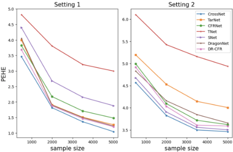
forms other competitive methods in both small sample and large sample scenarios across both two simulation settings.
4.3 Semi-synthetic Dataset: IHDP
We conduct experiments on the well known dataset IHDP created by [Hill, 2011], where the covariates are real and the outcomes are simulated. The dataset aims to evaluate the effect of home visit from specialist doctors on the cognitive test scores of premature infants. There are 747 units (139 in treated group and 608 in control group) and 25 real covariates, with 6 being continuous and 19 being binary, measuring the features of children and their mothers. We use the same version as in [Curth and van der Schaar, 2021], that is the setting "B" described in [Hill, 2011], where the outcomes are simulated by Y (0) ∼ N(exp ((X +W)βB) , 1) and Y (1) ∼ N(XβB -ωsB , 1). βB is the coefficient vector with each entry being sampled from (0, 0.1, 0.2, 0.3, 0.4) with probabilities (0.6, 0.1, 0.1, 0.1, 0.1). We use the same 100 replications in [Shalit et al., 2017; Curth and van der Schaar, 2021]. Since we know the true treatment effect for all individuals, we use PEHE as the metric to evaluating the performance within-sample and out-of-sample. The results are shown in Table 1, from which we can see that our proposed approach has the best performance.
| METHODS | WITHIN-SAMPLE | OUT-OF-SAMPLE |
|---|---|---|
| TNET | 1.303± 0.097 | 1.311± 0.110 |
| TARNET | 1.294± 0.104 | 1.299± 0.113 |
| CFRNET | 1.156± 0.111 | 1.162± 0.118 |
| DRAGONNET | 1.188± 0.104 | 1.194± 0.112 |
| DR-CFR | 1.334± 0.072 | 1.342± 0.089 |
| SNET | 1.354± 0.061 | 1.366± 0.081 |
| CROSSNET | 1.077± 0.064 | 1.084± 0.068 |
| METHODS | WITHIN-SAMPLE | OUT-OF-SAMPLE |
|---|---|---|
| TNET | 0.131± 0.002 | 0.173± 0.009 |
| TARNET | 0.119± 0.009 | 0.139± 0.001 |
| CFRNET | 0.111± 0.004 | 0.140± 0.008 |
| DRAGONNET | 0.120± 0.009 | 0.139± 0.006 |
| DR-CFR | 0.117± 0.008 | 0.138± 0.008 |
| SNET | 0.128± 0.007 | 0.149± 0.005 |
| CROSSNET | 0.109± 0.003 | 0.123± 0.004 |
4.4 Real Dataset: Jobs
We also apply our approach to the Job dataset first analyzed by [LaLonde, 1986]. The study aims to evaluating the effect of job training on income and employment status. Following [Smith and Todd, 2005; Shalit et al., 2017], we also consider the binary classification task for unemployment. This study contains experimental sample and the PSID comparison group. We split the dataset into train/validation/test sets and repeat 10 times to take average of the results. Since we do not know the true treatment effect, we can not calculate PEHE here. We use another metric defined in [Shalit et al., 2017], called policy risk. For a model f, the policy risk is R(f) = 1 - (E[Y1|πf (x) = 1] · p(πf = 1) + E[Y0|πf (x) = 0] · p(πf = 0)), where πf (x) = 1 if f(x, 1) - f(x, 0) > λ, and πf(x) = 0 otherwise. The policy risk measures the average loss in outcome when using the treatment policy estimated by the model. The results are shown in Table 2, and our approach has the smallest policy risk.
5 Conclusion
In this paper we propose a novel neural network approach for estimating CATE. We learn a sufficient representation that satisfies the unconfoundedness assumption by imposing a penalty on the discrepancy between the conditional distributions of two potential outcomes based on the representation under treatment and control, making the final treatment effect estimation more reasonable and effective. Another advantage of this architecture is that it allows the data from different groups to participate in the training of the hypothesis function of the other group, making h1 and h0 more applicable to the data from the other group, thereby mitigating the issue of selection bias. That is, the training of the hypothesis function for the treatment group no longer relies solely on minimizing the factual loss of the treated group; it also takes into account the ability to obtain better counterfactual predictions for the control group's data. This principle applies to the control group as well, thus we fully utilize the information from the samples to learn more robust hypothesis functions. We apply our approach to synthetic dataset, semi-synthetic dataset, real dataset and achieve good performance on all of them.
Acknowledgments
This work is supported by Ant Group Research Intern Program. This work is also supported by National key R&D Programmes of China (2022YFA1003800), National Statistical Science Research Grants of China (2022LD08), the National Natural Science Foundation of China (12231011, 71988101, 71925007 and 72091212), the CAS Project for Young Scientists in Basic Research (YSBR-008).
@inproceedings{ijcai2024p541,
  title     = {Estimating Conditional Average Treatment Effects via Sufficient Representation Learning},
  author    = {Shi, Pengfei and Zhong, Wei and Zhang, Xinyu and Wang, Ningtao and Fu, Xing and Wang, Weiqiang and Jin, Yin},
  booktitle = {Proceedings of the Thirty-Third International Joint Conference on
               Artificial Intelligence, {IJCAI-24}},
  publisher = {International Joint Conferences on Artificial Intelligence Organization},
  editor    = {Kate Larson},
  pages     = {4894--4901},
  year      = {2024},
  month     = {8},
  note      = {Main Track},
  doi       = {10.24963/ijcai.2024/541},
  url       = {https://doi.org/10.24963/ijcai.2024/541},
}
TY - CPAPER TI - Estimating Conditional Average Treatment Effects via Sufficient Representation Learning AU - Shi, Pengfei AU - Zhong, Wei AU - Zhang, Xinyu AU - Wang, Ningtao AU - Fu, Xing AU - Wang, Weiqiang AU - Jin, Yin T2 - Proceedings of the Thirty-Third International Joint Conference on Artificial Intelligence, IJCAI-24 PB - International Joint Conferences on Artificial Intelligence Organization PY - 2024 SP - 4894 EP - 4901 DO - 10.24963/ijcai.2024/541 UR - https://doi.org/10.24963/ijcai.2024/541 ER -Copied
Machine-readable versions of this paper, for tools and AI agents:





