Learning with Posterior Sampling for Revenue Management under Time-varying Demand

1 Introduction andMotivation

Maximizing revenue by pricing items or services is a key problem in many industries such as airline and retail industries. This kind of problem is known as a price-based revenue management (RM) problem, which has been extensively studied in operations research and management science. To determine optimal prices, it is essential to capture the relation between the selling price and demand, which is called a demand curve. However, in the real world, such a curve is not only unavailable to a seller in advance, but is also stochastic.

∗He is currently affiliated with the University of Tokyo.

Thus, maximizing revenue in real-world businesses requires the seller to deal with both unknown and stochastic demand.

Another challenge in the RM problem is that demand may depend not only on the offered price but also on the time. Such a dynamic nature of the demand can particularly appear in applications where sold items or services have some deadlines [Gallego and Van Ryzin, 1997; Su, 2007]. For example, more business trippers reserve airplane seats as the departure date approaches as their schedules become clearer [Lazarev, 2013; Williams, 2020].

Despite its potential importance of addressing such dynamic demand, most studies on RM problems with unknown demand have focused on the stationary demand whose distribution solely depends on the price. This discrepancy might come from the typical formulation of the problem, where a seller experiences a single selling season. In such a scenario, the seller can observe the actual demand for each time period only once, and thus it is impossible to correctly estimate the future demand from the observed one. One could mitigate this limitation if some model on the time dependency of the demand is assumed. Still, it is not realistic to construct a model that precisely predicts future demands since the demand often drastically changes especially around the end or start of selling seasons. Su [2007] discusses this dynamic demand changes in the fashion and travel industries.

A clue to address this difficulty from the practical viewpoint is that a seller often has multiple seasons to sell items or services with an independent amount of inventories. In the case of the hotel industry, for example, the demands for rooms of the same day of the week almost do not vary among weeks unless there is a special event near the hotel [Bandalouski et al., 2021]. Thus, the seller can learn demand for rooms by pricing them across multiple weeks.

In consideration of such applications, we introduce a generalization of the RM problem, which we call an episodic price-based revenue management problem. In this problem, we consider the setting where selling seasons (or episodes) are repeated multiple times as follows. At the beginning of each selling season, a seller is given a fixed amount of inventory, which is not replenished during the season. At each time period of a season, the seller prices the item and the number of sold items is determined according to the demand whose distribution depends on the price and time period but is independent of the season.

In this episodic setting, we can learn the demand distribution depending on both the price and time period if we have infinitely many seasons. Our goal is to design a policy that efficiently explores the demand of each time period while exploiting the current knowledge to optimize the revenue in a finite number of seasons. Such exploration-exploitation tradeoff is much more complicated under the limited inventory with time-varying demand since the desired prices between different time periods affect each other through the inventory constraint and the prior model on the time-varying demand.

1.1 Our Contributions

For the proposed generalization of RM problems, we develop two algorithms that combine the pricing based on linear programming (LP) with the technique of posterior sampling called Thompson sampling [Thompson, 1933] in online-learning. This combination successfully leads to balancing the exploration-exploitation trade-off with inventory constraint to efficiently achieve high performance.

The first algorithm, TS-episodic, determines the schedule of prices during a season at the beginning of each season, which is computationally efficient while having a reasonable theoretical guarantee. The second algorithm, TS-dynamic, is a heuristic modification of TS-episodic, which dynamically updates the pricing at each time period of a season. This modification can quickly reflect the observed data in the prices and enables robustness to stochastic demand. We numerically demonstrate that the proposed algorithms become close to the oracle policy that is optimal in hindsight as the number of seasons increases, and this convergence is particularly fast under TS-dynamic.

On the theoretical contributions, we derive both upper and lower bounds on Bayesian regret. We first derive an upper bound on the Bayesian regret for TS-episodic of O(T √SK log(K) + S√T), where S is the number of episodes, T is the selling horizon (the number of time periods) of each episode, and K is the number of feasible prices. We also derive a Bayesian regret lower bound for generic algorithms of Ω(T √SK). The regret upper bound is sublinear in the total number ST of time steps when S and T jointly increase. In particular, the first term O(T √SK) matches the lower bound up to a logarithmic factor and is unavoidable. The second term is linear in S, which can be regarded as a cost for computational efficiency coming from the fact that the optimal pricing needs a dynamic programming with a very large table even if the seller completely knows the demand distributions. This kind of linear regret often appears in the settings where the problem involves a complicated optimization problem (see the discussion below Theorem 1).

1.2 Literature Review and Distinctions

The literature on RM problems primarily focuses on cases with known demand information. In such settings, RM problems with dynamic demand are well investigated [Gallego and Van Ryzin, 1994; Gallego and Van Ryzin, 1997; Zhao and Zheng, 2000; Anjos et al., 2005; Malighetti et al., 2009]. Other topics of price-based RM problems are reviewed in Bitran and Caldentey [2003]; Chiang et al. [2007].

RM problems with demand learning are studied later, which are reviewed in Den Boer [2015]. In addition, there exist other types of revenue management problems called quantitybased revenue management. We refer the reader to Strauss et al. [2018]; Klein et al. [2020] and references therein for recent developments in such RM problems.

The episodic RM problem is related to reinforcement learning (RL) in a time-inhomogeneous Markov decision process (MDP) [Hao and Lattimore, 2022; Moradipari et al., 2023]. The regret analysis of the RL literature typically relies on an oracle to exactly compute the optimal pricing policy whereas our algorithms use LP for computational efficiency. This difference requires us to carefully evaluate the gap between the optimal pricing schedule and the approximated schedule by LP as will be discussed in Section 3.

For other episodic settings, den Boer and Zwart [2015] discuss an episodic RM for unknown stationary demand. In addition, Chen et al. [2022] consider a related episodic setting with unknown non-stationary demand. However, their setting allows inventory shortages (negative inventory) with a small extra cost, 1 meaning that inventory shortage does not drastically affect the revenue unlike our setting. Furthermore, their algorithm relies on more restricted demand conditions than ours, such as a sub-Gaussian demand distribution.

The most closely related work is Ferreira et al. [2018], which focuses on a generalization of a RM problem with unknown stationary demand. They provide algorithms based on Thompson sampling that balance the exploration-exploitation trade-off under inventory constraints. They derive upper bounds of Bayesian regret for their algorithms and demonstrate their outstanding performance in numerical experiments. However, their algorithms heavily rely on the stationary demand setting, and extending them to non-stationary settings is highly non-trivial.

2 Problem Setting

In this section, we formulate the episodic RM problem and propose algorithms with posterior sampling.

2.1 Revenue Management Process

We consider the setting where a seller deals in a single item and repeats selling seasons S times. Each selling season, indexed by s ∈ [S] = {1, 2, . . . , S}, consists of T ∈ Z time periods. At the beginning of each selling season, the seller has n0 units of initial inventory, which is not replenished during the selling season. The inventory at the end of period t is denoted by nt;s, and n0;s = n0. Each time period t ∈ [T ] of the s-th season consists of the following procedures:

(i) The seller chooses a price Pt;s from the set of K + 1 prices P ∪ {p∞}. Here, P = {pk}k∈[K] ∈ [0,∞)K is a set of feasible prices and p∞ is a "shut-off" price, which is commonly used in dynamic pricing literature. Under the shutoff price p∞, the demand is zero and no revenue is obtained with probability one.

1 To be more specific, Chen et al. [2022] consider the setting where the cost is incurred depending on the possibly negative remaining inventory at the end of the episode, and this cost is Lipschitz continuous in the remaining inventory.

• (ii) The seller observes random demand Dt;s ≥ 0 that is independent of the past prices and demands. The distribution under the offered price pk is denoted by Dt,k(θ), where θ ∈ Θ is a parameter unknown to the seller.
• (iii) The inventory is consumed according to the observed demand Dt;s to yield revenue. The seller can consume at most nt-1;s units of the inventory and the inventory at the end of the current time period is expressed as nt;s = max(nt-1;s - Dt;s, 0), which yields revenue Pt;s min(Dt;s, nt-1;s).

Remark 1. This formulation considers the case where there are units of only one item to sell, whereas Ferreira et al. [2018] consider the case of multiple items. We focus on the case of a single item just to highlight the difficulty of the dynamic demand although the extension to the case of multiple items is straightforward as discussed in Appendix F.

We adapt a Bayesian approach in our demand model. We assume that a demand parameter θ ∈ Θ follows some given prior distribution f. For any t ∈ [T] and s ∈ [S], the posterior distribution is determined by the history Hs t-1 of offered prices and observed demands up to the current time period of the season, which is expressed as Hs t-1 = {(Pτ;σ,Dτ;σ)}τ∈[T],σ∈[s-1] ∪ {(Pτ;s,Dτ;s)}τ∈[t-1]. Given a history Hs t-1 , the posterior distribution is then expressed as f (θ|Hs t-1 ) ∝ P(Hs t-1 |θ)f(θ), where P(Hs t-1 |θ) is the likelihood function.

Note that we impose no assumption on the demand model {Dt,k(θ)}t∈[T],k∈[K],θ∈Θ and the prior distribution f(θ) as far as f is a well-defined probability distribution (that is, an improper prior in the Bayesian statistics is not used). In particular, we allow models where the demands among different prices and time periods are correlated. This is a special strength of our framework capturing wide models, while causing technical difficulties since the estimator or the posterior distribution of the demand at each price and time period might complicatedly depend on the past observations. We introduce two examples of demand models below, both of which are used in the numerical analysis in Section 4.

Example 1 (Poisson Demand with Independent Gamma Priors). This is a simple model of the demand distributions, in which the demand distribution Dt,k(θ) is expressed as Dt,k(θ) = Poi(·|λt,k) for k ∈ [K] and time t ∈ [T], where Poi(·|λ) is a Poisson distribution with intensity λ ∈ R+. The intensity parameters {λt,k}t∈[T],k∈[K] are assumed to be independently and identically distributed by gamma distributions Ga(α, β) with shape α > 0 and scale β > 0. Since gamma distributions are conjugate to Poisson distributions, the posterior distribution remains a gamma distribution that can be easily computed. Still, this model requires estimation of KT parameters θ = {λt,k}k∈[K],t∈[T ] independent of each other and is not always sample-efficient in realistic settings.

Example 2 (Poisson Demand with Gaussian Process Prior). In this model, Dt,k(θ) = Poi(·|λt,k) is assumed as in the first example, but the intensity parameters {λt,k}t∈[T ],k∈[K] are modeled using a Gaussian process. To be more specific, this model assumes that the intensity parameter is expressed as λt,k = exp(g(t, pk)) > 0 for g(t, p) : [T] × P → R following a Gaussian process with some mean function µ(·) : [T ] × P → R and kernel function K(·, ·) : ([T] ×P) × ([T] ×P) →R. Under this model, the posterior distribution of {λt,k}t∈[T ],k∈[K] has no closed form but it can be approximated by, e.g., Laplace approximation and Markov chain Monte Carlo method (see Appendix H.2 and Rasmussen and Williams [2005] for further details).

2.2 Proposed Algorithms

For the problem we stated so far, we propose two algorithms, TS-episodic and TS-dynamic. These algorithms use a mean demand function for a demand parameter θ ∈ Θ, which is defined as

With this mean demand function, the proposed algorithms solve the linear optimization problem LP(θ, t, n) over {xτ,k}t≤τ≤T, k∈[K] ∈ [0, 1](T-t+1)K , defined as follows:

In this problem, xτ,k intuitively corresponds to the probability of choosing price pk at time period τ. This optimization problem corresponds to a kind of LP relaxation of the revenue optimization problem in our setting. To be more specific, if the domain of {xτ,k}t≤τ≤T, k∈[K] is restricted to be binary and Dt,k is deterministic then (1) gives the optimal pricing policy under a parameter θ when the inventory is n at time period t. We use {xτ,k(θ)}t≤τ≤T,k∈[K] to denote the optimal solution of LP(θ, t, n).

Although relying on linear programming instead of dynamic programming may result in a suboptimal algorithm, LP is commonly used particularly in bandit with knapsack problems for both stationary and non-stationary settings (see, for example, Badanidiyuru et al. [2013]; Immorlica et al. [2022]; Liu et al. [2022]).

The first algorithm, TS-episodic, is given in Algorithm 1. At the beginning of the selling season, this algorithm randomly samples a demand parameter θs from its posterior distribution. Then, the algorithm solves the LP(θs, 1, n0) to obtain a solution {xτ,k(θs)}τ∈[T ],k∈[K]. At every time period t, TS-episodic randomly chooses the prices according to this solution computed at the beginning of the season.

The second algorithm, TS-dynamic, samples a parameter θt;s and solves LP(θt;s, t, nt-1;s) at every time period. The algorithm then determines the price according to xt,k(θt;s). These procedures enable us to immediately exploit the demand observation at each time period.

TS-episodic has a simpler structure than TS-dynamic since TS-episodic samples a demand parameter and solves the LP only once at the beginning of each episode, whose solution is used throughout the season. Still, due to the randomness of the offered price and the demand, the remaining

Algorithm 1: TS-episodic

1 for s = 1, . . . , S do 2 Sample a demand parameter θs ∈ Θ from the posterior distribution f(·|Hs 0 ) of θ. 3 Solve LP(θs, 1, n0). 4 for t = 1, . . . , T do 5 Offer price Pt;s = pk with probability xk,t(θs) and Pt;s = p∞ with probability 1 - ∑Kk=1 xt,k(θs). 6 Observe realized demand Dt;s and update the history as Hs t =Hs t-1 ∪ {Pt;s, Dt;s}.

Algorithm 2: TS-dynamic

1 for s = 1, . . . , S do 2 for t = 1, . . . , T do 3 Sample a demand parameter θt;s ∈ Θ from the posterior distribution f(·|Hs t-1 ) of θ. 4 Solve LP(θt;s, t, nt-1;s). 5 Offer price Pt;s = pk with probability xk,t(θt;s) and Pt;s = p∞ with probability 1 - ∑Kk=1 xt,k(θt;s). 6 Observe realized demand Dt;s and update the history Hs t =Hs t-1 ∪ {Pt;s, Dt;s}.

inventory sometimes becomes unstable, which might cause discrepancy from the optimal pricing policy. TS-dynamic, on the other hand, samples the demand parameter and solves the LP based on the current inventory at each time period. It thus can dynamically control the inventory during a selling season, and can immediately exploit the demand information soon after the observation. These properties possibly enable TS-dynamic to learn demand faster than TS-episodic and to have better performance at the cost of the computational time about T times larger than that of TS-episodic.

The proposed algorithms balance the explorationexploitation trade-off through the randomness of the samples from the posterior distribution with pricing by LP. In particular, the important characteristic of the proposed algorithms is that the future demand is taken into account through the LP when determining the price for the current time period. Although pricing by LP is also considered in Ferreira et al. [2018], it assigns the inventory uniformly into each time period, which results in no more optimal revenue under the time-varying demand. This difference is drastically reflected in the performances of the proposed algorithms and benchmarks as shown in Section 4.

3 Regret Analysis

In this section, we first analyze the Bayesian regret of TSepisodic and then derive a Bayesian regret lower bound for generic algorithms. The problem-dependent regret is the difference between the total expected revenue obtained by the algorithm and that by the optimal policy π∗ (θ) in hindsight, which is defined as follows.

Definition 1. The problem-dependent regret of an algorithm π under a demand parameter θ ∈ Θ is

Here, the optimal pricing policy in hindsight π∗ (θ) serves as a chosen competitive algorithm. We then define the Bayesian regret as the expectation of the problem-dependent regret with respect to a prior distribution f over θ.

Definition 2. The Bayesian regret of an algorithm π for a prior f is

where Eθ[·] denotes the expectation taken for θ following f.

The Bayesian regret is a typical performance measure of online Bayesian algorithms. See Russo and Van Roy [2014] for further interpretations of Bayesian regret.

Theorem 1. Assume that 4K ≤ S and there exists ¯ d > 0 such that the support of the distribution Dt,k(θ) is finite and included in [0, ¯ d] for all θ. Then, the Bayesian regret (3) of TS-episodic satisfies

From the upper bound of this theorem, we see that the regret is sublinear in ST when S and T jointly increase. Here the first term of O(S√T) is linear in S but it can be regarded as a cost for computational efficiency. Even if we know the true demand parameter θ, the optimal pricing policy π∗ (θ) requires to compute dynamic programming, which is sometimes costly in practice though it is polynomial time. Furthermore, the optimal pricing policy π∗ (θ) essentially depends on the demand distributions {Dt,k(θ)}t,k themselves rather than their expectations. On the other hand, the proposed algorithms use the linear programming, which can be computed efficiently in practice by off-the-shelf solvers, and behave stably since we only need to estimate the expected demands.

Note that this kind of linear regret often implicitly appears in the online learning problems involving complicated optimization problems. In such problems, the notion of α-regret is often introduced instead, which corresponds to the regret when the optimal algorithm π∗ (θ) in (2) is replaced with an approximate algorithm with approximation ratio of α [Garber, 2017; Wen et al., 2017]. The regret of O(S√T) corresponds to this gap between the optimal policy π∗ (θ) and the approximation algorithm based on LP(θ, 1, n0) for the true parameter θ.

Remark 2. The linear termmight be avoidable if we exactly optimize the pricing schedule by dynamic programming instead of LP and combine techniques in RL literature. They often consider the regret analysis under exact optimization of the schedule, which might be applicable if we regard our problem as an MDP. However, such an analysis is highly non-trivial since our model allows complex prior distributions unlike existing studies of RL literature that focus on independent or specific prior distributions [Osband and Van Roy, 2017; Lu and Van Roy, 2019; Hao and Lattimore, 2022; Moradipari et al., 2023].

Key Points in the Proof of Theorem 1. The key challenge in the analysis of Theorem 1 is that the inventory constraint affects the offered prices and the total revenue in a very complicated way, through the dynamic programming in the optimal policy in hindsight and the LP in the proposed policy. Due to this challenge, standard regret analysis approaches for Thompson sampling algorithms, such as the one in Russo and Van Roy [2014], cannot be directly applied to our problem. Though the inventory constraint is already considered in Ferreira et al. [2018], their argument is limited to the static demand because the best policy is to uniformly assign the inventory to each time period. To address this difficulty with the inventory constraint, we employ an approach to reduce the problem into T instances of MAB problems with K arms and S rounds. These T problems are highly correlated through the inventory constraint and the posterior distribution, but we show by a careful analysis that the regret can be decomposed into that of T independent instances and that arising from the correlation. We will give more details of the proof in Section 3.1 (the formal proof is given in Appendix D).

The following theorem ensures that the second term O(T √SK logK) of the regret upper bound in Theorem 1, which is linear in T, is essential in the Bayesian regret:

Theorem 2. Assume the same condition as that in Theorem 1 and n0 ≥ ¯ d. Then, there exists a demand model {Dt,k(θ)}t∈[T],k∈[K],θ∈Θ and a prior distribution f0 over Θ such that the Bayesian regret (3) of any algorithm π satisfies

Key Points in the Proof of Theorem2. Themain difficulty in deriving this lower bound arises from the inventory constraint, which can vary the optimal price depending on the remaining inventory. This prohibits the use of common toolkits for evaluating lower bounds in multi-armed bandit problems. To address this challenge, we provide an instance where demand can appear in chosen m = ⌈ n0 ¯ d ⌉ time periods and no demand in other time periods. This setting decomposes our problem into m independent dynamic pricing tasks since the inventory never runs out. For each of the m tasks, we can then use techniques for lower bound analysis of MAB problems (see, for example, Section 15 of Lattimore and Szepesv´ari [2020]). These techniques provide potential instances where any algorithm must incur at least Ω(√SK) regret. The existence of such instances for each of the m tasks allows us to choose a prior distribution f for which the Bayesian regret is bounded below for any algorithms. The formal proof of Theorem 2 is given in Appendix E.2.

3.1 Proof Sketch of Theorem 1

First, we decompose the expected total revenue Revπ (T, S, θ) into the (virtual) total revenue ignoring the inventory limit and the lost sales due to the lack of inventory. To be more specific, we decompose the regret by

BRegret(T, S, f, π)

We refer to the underlined parts (A) and (B) as the revenuedifference and the lost sales parts, respectively. In the rest of this section, we will briefly sketch the derivation of upper bounds for these revenue-difference and lost sales parts. In what follows, we will use the notation Eπ [·] = Eθ [Eπ [·|θ]].

Evaluation of the Revenue-difference Part

As we will show in Lemma 14 in Appendix C.6, Rev∗ (T, θ) is bounded above by the optimal value of LP(θ, 1, n0). This fact allows us to have

However, the right-hand side of this inequality remains difficult to analyze since the solution of the LP depends on the inventory allocation across time periods.

To address this difficulty related to the complex inventory allocation, we introduce a set of upper confidence bounds {Ut,k;s}t∈[T],k∈[K],s∈[S] (the definition of Ut,k;s is given in Appendix B). The upper confidence bound Ut,k;s bounds the mean demand λt,k(θ) above with high probability. By combining these upper confidence bounds and the regret decomposition technique of Russo and Van Roy [2014], we have

For any fixed t ∈ [T] and k ∈ [K], Ut,k;s will decrease and converge to λt,k(θ) as the k-th price is offered. Thus, both (λt,k(θ) - Ut,k;s) xt,k(θ) and (Ut,k;s - λt,k(θ)) xt,k(θs) can vanish as the number of seasons increases, which eventually results in an upper bound for (A):

The complete argument to derive this bound is given in the proof of Lemma 15 in Appendix C.6.

Evaluation of the Lost Sales Part

x+ = max{x, 0}, and the detailed derivation is in Appendix D. This expectation is further bounded by

where the inequality follows from (x + y)+ ≤ x+ + y+. The underlined part (B1) is bounded above by the conditional variance of ∑Tt=1 Dt;s on θ from the Cauchy-Schwarz inequality, EX[|X|]2 ≤ EX[X2 ]. (B1) is then bounded by an upper bound of the variance ¯ d√T . Then, we have

For the underlined part (B2), recall that the solution of LP(θt, 1, n0) satisfies ∑Tt=1 ∑Kk=1 λt,k(θs)xt,k(θs) ≤ n0 due to the inventory constraint. Combining this relation with Eπ [ ∑Tt=1 Dt;s ∣∣∣ θ] = ∑Kk=1 ∑Tt=1 λt,k(θ)xt,k(θs), we have

Following a similar argument to that used in the derivation of (5), we obtain(B2) ≤ ¯ d (36T √SK log(K)) . (7)

The detailed derivation of this bound is given in Lemma 13 in Appendix C.5.

From (5), (6) and (7), we can bound (A) and (B) in (4) and thus have proved Theorem 1.

Remark 3. Proving a theoretical upper bound is more challenging for TS-dynamic than for TS-episodic. This is because TS-dynamic repeatedly solves LP and the resulting total revenue depends on dynamical changes in remaining inventory. This distinction complicates the regret analysis, which requires a new technique for theoretical analyses. However, we believe that TS-dynamic could have a theoretical bound of the Bayesian regret with the same order as that of TS-episodic due to its using LP and the lower bound in Theorem 2. The additional evidence of this belief is the empirical results presented in Section 4, where there is no significant difference in the performance between the two algorithms.

4 Experiments

In this section, we show numerical results 2 on the expected regret of the proposed algorithms and benchmark ones. Additional results are given in Appendix G.

2 The code of the experiments is available at: https://github.com/ NECDSresearch2007/RM-TSepisodic-and-dynamic.

Experimental Settings We consider the set of K = 9 prices P = {1, 2, . . . , 9} with a shut-off price p∞. The selling horizon is set to T = 10. The true demand distribution is set to Poisson distributions with mean demand parameters λ(t, p) = 50 exp (- p+t 5 ), depending on the time t and price p. These demand parameters can be viewed as an exponential-type demand curve [Gallego and Van Ryzin, 1994] with an exponentially decreasing coefficient with time, which results in the discounted revenue case [Gallego and Van Ryzin, 1997]. The initial inventory is set to n0 = 1000 and 50, corresponding to the cases where there is enough inventory and where the inventory is quite limited, respectively. In the former setting, pricing can be made almost independently between time periods and the problem becomes easier.

For the prior on the demand distributions in the proposed algorithms and benchmarks, we used the two models discussed in Examples 1 and 2, respectively. The details of these priors are as follows.

Independent Gamma Prior: For Example 1 in Section 2.1, we set prior gamma distributions with shape α = 10 and scale β = 1 for all k ∈ [K] and t ∈ [T ].

Gaussian Process (GP) Prior: For Example 2 in Section 2.1, we took the mean function µ as a zero function and the kernel function as an anisotropic radial basis function kernel defined as, K ((p, t), (p′ , t′ )) = exp (-(t - t′ )2 /σ2 t - (p - p′ )2 /σ2 p ) where σt = 3 σp = 2.5.

We consider the number of episodes S = 5000 for the settings with the independent gamma prior (referred to as independent prior hereafter) and S = 200 for the GP prior. We run independent 100 trials for each setting.

Comparison Targets In the considered setting, we can compute the optimal policy π∗ (θ) using the dynamic programming in manageable time though not practically efficient. Then, we measure the performance of the algorithms based on the relative ratio of the cumulative revenue compared with π∗ (θ).

We compared the performance of the proposed algorithms with four benchmark algorithms. The first two algorithms are generalizations of TS-fixed and TS-update in Ferreira et al. [2018] to our problem, which are denoted by TS-fixed* and TS-update*, respectively. To measure the gap between the performance of the optimal policy π∗ (θ) and the policy based on linear relaxation, we also consider two oracle algorithms, which are denoted by TS-episodic* and TSdynamic*. In these algorithms, the true demand parameter is used instead of the one sampled from the posterior. Then, TS-episodic* and TS-dynamic* are independent of episodes and Bayesian settings by production. We compute their regret in an episode over 10000 trials. The details of these benchmarks are given in Appendix H.1.

Numerical Results Figure 1 provides numerical results of the relative expected regrets 1 - Revπ (T, s, θ) / (sRev∗ (T, θ)) for s ∈ [S].

For the case of n0 = 1000 shown in Figures 1 (A2) and (B2), our proposed algorithms and the benchmark algorithms show almost the same performance. This is because greedily optimizing the price at each round leads to the optimal policy and all the algorithms can learn efficient pricing without considering the inventory allocation across time periods.

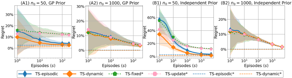
Figures 1 (A1) and (B1) show the results for the case of n0 = 50. They demonstrate that the proposed algorithms can successfully learn an efficient pricing policy to maximize total revenue over the selling season unlike the benchmark algorithms. In particular, TS-dynamic learns an efficient pricing policy faster than TS-episodic and shows better performance as expected.

The results for TS-episodic* and TS-dynamic* in Figure 1 for n0 = 50 show that their expected regret does not become zero even under the knowledge of the true demand parameters, which corresponds to the term O(S√T) in the regret bound in Theorem 1, which is linear in S. This is the inevitable cost of relying on the linear optimization instead of dynamic programming.

Remark 4. Whereas TS-dynamic learns an efficient policy faster than TS-episodic, dynamically recomputing LP does not always contribute to a better allocation after demand parameters are learnt well. In fact, we give a result in Appendix G where TS-dynamic* becomes slightly worse than TS-episodic* in certain settings. In this way, behavior of the allocation based on LP relaxation with recomputation becomes complicated even under known parameters, which makes the analysis of TS-dynamic particularly difficult.

We next discuss the effect of prior distributions. Our proposed algorithms with both the independent prior and the GP prior achieve almost the same performance level around the final episode. However, the algorithms with the independent prior spend more episodes to learn an efficient pricing policy than the ones with the GP prior. This result arises from the prior model where the mean demand function {λt,k(θ)}t∈[T],k∈[K] must be independently estimated. In contrast, our algorithms under the GP prior can learn faster through the kernel function utilizing the dependency of the demands between time periods.

5 Conclusion

In this paper, we investigated a price-based revenue management problem, in which a seller tries to maximize the total revenue over a finite selling season with finite inventory of an item. In particular, we considered the episodic scenario with unknown and time-varying demand with the real-world applicability in mind. For this problem, we proposed TSepisodic, which combines the pricing based on linear programming relaxation with posterior sampling. We derived a regret guarantee for TS-episodic and confirmed its effectiveness by numerical simulation. We also proposed TSdynamic, which is a heuristic modification of TS-episodic and dynamically updates the posterior sample and the pricing. We numerically confirmed this algorithm can further quickly learn an effective pricing policy.

Finally, we present two relevant future directions. The first direction is to find an algorithm that can achieve an upper bound of the Bayesian regret without the O(S√T) term. Such an algorithm would need to minimize lost sales as much as the optimal policy in hindsight does. The other direction is to find a precise theoretical analysis for TS-dynamic. However, this direction is challenging due to the difficulty of analyzing the algorithm repeating LP even if the true demand parameters are known as in TS-dynamic*. Therefore, it may be possible to analyze the difference of the regret of TSdynamic compared with TS-dynamic* instead of that with the optimal hindsight policy, π∗ (θ).

Acknowledgements

The authors appreciate helpful and constructive comments for the anonymous reviewers. JH was supported by JSPS, KAKENHI Grant Number JP21K11747, Japan.