
Subgraph Pooling: Tackling Negative Transfer on Graphs
Proceedings of the Thirty-Third International Joint Conference on Artificial Intelligence. Main Track. Pages 5153-5161.
https://doi.org/10.24963/ijcai.2024/570
Keywords
- Machine Learning: ML: Sequence and graph learning
- Machine Learning: ML: Semi-supervised learning
- Machine Learning: ML: Multi-task and transfer learning
- Data Mining: DM: Mining graphs
Abstract
Transfer learning aims to enhance performance on a target task by using knowledge from related tasks. However, when the source and target tasks are not closely aligned, it can lead to reduced performance, known as negative transfer. Unlike in image or text data, we find that negative transfer could commonly occur in graph-structured data, even when source and target graphs have semantic similarities. Specifically, we identify that structural differences significantly amplify the dissimilarities in the node embeddings across graphs. To mitigate this, we bring a new insight in this paper: for semantically similar graphs, although structural differences lead to significant distribution shift in node embeddings, their impact on subgraph embeddings could be marginal. Building on this insight, we introduce Subgraph Pooling (SP) by aggregating nodes sampled from a k-hop neighborhood and Subgraph Pooling++ (SP++) by a random walk, to mitigate the impact of graph structural differences on knowledge transfer. We theoretically analyze the role of SP in reducing graph discrepancy and conduct extensive experiments to evaluate its superiority under various settings. The proposed SP methods are effective yet elegant, which can be easily applied on top of any backbone Graph Neural Networks (GNNs). Our code and data are available at: https://github.com/Zehong-Wang/Subgraph-Pooling.
- [Cao et al., 2023] Yuxuan Cao, Jiarong Xu, Carl Yang, Ji- aan Wang, Yunchao Zhang, Chunping Wang, Lei CHEN, and Yang Yang. When to pre-train graph neural networks? from data generation perspective! In KDD, 2023.
- [Chen et al., 2022] Yongqiang Chen, Yonggang Zhang, Yatao Bian, Han Yang, MA Kaili, Binghui Xie, Tongliang Liu, Bo Han, and James Cheng. Learning causally in- variant representations for out-of-distribution generaliza- tion on graphs. NeurIPS, 2022.
- [Chuang and Jegelka, 2022] Ching-Yao Chuang and Ste- fanie Jegelka. Tree mover's distance: Bridging graph met- rics and stability of graph neural networks. In NeurIPS, 2022.
- [Dai et al., 2022a] Enyan Dai, Wei Jin, Hui Liu, and Suhang Wang. Towards robust graph neural networks for noisy graphs with sparse labels. In WSDM, 2022.
- [Dai et al., 2022b] Quanyu Dai, Xiao-Ming Wu, Jiaren Xiao, Xiao Shen, and Dan Wang. Graph transfer learning via adversarial domain adaptation with graph convolution. TKDE, 2022.
- [Fey and Lenssen, 2019] Matthias Fey and Jan Eric Lenssen. Fast graph representation learning with pytorch geometric. arXiv, 2019.
- [Ganin et al., 2016] Yaroslav Ganin, Evgeniya Ustinova, Hana Ajakan, Pascal Germain, Hugo Larochelle, Franc ¸ois Laviolette, Mario March, and Victor Lempitsky. Domain- adversarial training of neural networks. JMLR, 2016.
- [Gaudelet et al., 2021] Thomas Gaudelet, Ben Day, Arian R Jamasb, Jyothish Soman, Cristian Regep, Gertrude Liu, Jeremy BR Hayter, Richard Vickers, Charles Roberts, Jian Tang, et al. Utilizing graph machine learning within drug discovery and development. Briefings in bioinformatics, 2021.
- [Gretton et al., 2006] Arthur Gretton, Karsten Borgwardt, Malte Rasch, Bernhard Schölkopf, and Alex Smola. A ker- nel method for the two-sample-problem. NeurIPS, 2006.
- [Gui et al., 2022] Shurui Gui, Xiner Li, Limei Wang, and Shuiwang Ji. GOOD: A graph out-of-distribution bench- mark. In NeurIPS, 2022.
- [Guo et al., 2023] Yuxin Guo, Cheng Yang, Yuluo Chen, Jixi Liu, Chuan Shi, and Junping Du. A data-centric framework to endow graph neural networks with out-of- distribution detection ability. In KDD, 2023.
- [Hamilton et al., 2017] Will Hamilton, Zhitao Ying, and Jure Leskovec. Inductive representation learning on large graphs. In NeurIPS, 2017.
- [Han et al., 2021] Xueting Han, Zhenhuan Huang, Bang An, and Jing Bai. Adaptive transfer learning on graph neural networks. In KDD, 2021.
- [Han et al., 2022] Xiaotian Han, Zhimeng Jiang, Ninghao Liu, and Xia Hu. G-mixup: Graph data augmentation for graph classification. In ICML, 2022.
- [He et al., 2020] Xiangnan He, Kuan Deng, Xiang Wang, Yan Li, Yongdong Zhang, and Meng Wang. Lightgcn: Simplifying and powering graph convolution network for recommendation. In SIGIR, 2020.
- [Hu et al., 2020] Weihua Hu, Matthias Fey, Marinka Zitnik, Yuxiao Dong, Hongyu Ren, Bowen Liu, Michele Catasta, and Jure Leskovec. Open graph benchmark: Datasets for machine learning on graphs. In NeurIPS, 2020.
- [Huang et al., 2021] Zexi Huang, Arlei Silva, and Ambuj Singh. A broader picture of random-walk based graph em- bedding. In KDD, 2021.
- [Huang et al., 2023] Wenbing Huang, Yu Rong, Tingyang Xu, Fuchun Sun, and Junzhou Huang. Tackling over- smoothing for general graph convolutional networks. TPAMI, 2023.
- [Jin et al., 2023] Wei Jin, Tong Zhao, Jiayuan Ding, Yozen Liu, Jiliang Tang, and Neil Shah. Empowering graph rep- resentation learning with test-time graph transformation. In ICLR, 2023.
- [Keriven, 2022] Nicolas Keriven. Not too little, not too much: a theoretical analysis of graph (over)smoothing. In LoG, 2022.
- [Kipf and Welling, 2017] Thomas N. Kipf and Max Welling. Semi-supervised classification with graph convolutional networks. In ICLR, 2017.
- [Lee et al., 2019] Junhyun Lee, Inyeop Lee, and Jaewoo Kang. Self-attention graph pooling. In ICML, 2019.
- [Levie et al., 2021] Ron Levie, Wei Huang, Lorenzo Bucci, Michael Bronstein, and Gitta Kutyniok. Transferability of spectral graph convolutional neural networks. JMLR, 2021.
- [Liu et al., 2020] Yanbei Liu, Xiao Wang, Shu Wu, and Zhi- tao Xiao. Independence promoted graph disentangled net- works. In AAAI, 2020.
- [Liu et al., 2022] Songtao Liu, Rex Ying, Hanze Dong, Lan- qing Li, Tingyang Xu, Yu Rong, Peilin Zhao, Junzhou Huang, and Dinghao Wu. Local augmentation for graph neural networks. In ICML, 2022.
- [Liu et al., 2023a] Shikun Liu, Tianchun Li, Yongbin Feng, Nhan Tran, Han Zhao, Qiang Qiu, and Pan Li. Structural re-weighting improves graph domain adaptation. In ICML, 2023.
- [Liu et al., 2023b] Yixin Liu, Kaize Ding, Huan Liu, and Shirui Pan. Good-d: On unsupervised graph out-of- distribution detection. In WSDM, 2023.
- [Long et al., 2018] Mingsheng Long, Zhangjie Cao, Jianmin Wang, and Michael I Jordan. Conditional adversarial do- main adaptation. In NeurIPS, 2018.
- [Ma et al., 2019] Jianxin Ma, Peng Cui, Kun Kuang, Xin Wang, and Wenwu Zhu. Disentangled graph convolutional networks. In ICML, 2019.
- [Mallinar et al., 2022] Neil Mallinar, James Simon, Amirhe- sam Abedsoltan, Parthe Pandit, Misha Belkin, and Pree- tum Nakkiran. Benign, tempered, or catastrophic: Toward a refined taxonomy of overfitting. In NeurIPS, 2022.
- [Qiu et al., 2020] Jiezhong Qiu, Qibin Chen, Yuxiao Dong, Jing Zhang, Hongxia Yang, Ming Ding, Kuansan Wang, and Jie Tang. Gcc: Graph contrastive coding for graph neural network pre-training. In KDD, 2020.
- [Ribeiro et al., 2017] Leonardo FR Ribeiro, Pedro HP Saverese, and Daniel R Figueiredo. struc2vec: Learning node representations from structural identity. In KDD, 2017.
- [Rozemberczki et al., 2021] Benedek Rozemberczki, Carl Allen, and Rik Sarkar. Multi-scale attributed node em- bedding. Journal of Complex Networks, 2021.
- [Ruiz et al., 2020] Luana Ruiz, Luiz Chamon, and Alejandro Ribeiro. Graphon neural networks and the transferability of graph neural networks. In NeurIPS, 2020.
- [Shi et al., 2023] Boshen Shi, Yongqing Wang, Fangda Guo, Jiangli Shao, Huawei Shen, and Xueqi Cheng. Improv- ing graph domain adaptation with network hierarchy. In CIKM, 2023.
- [Sun et al., 2023] Xiangguo Sun, Hong Cheng, Jia Li, Bo Liu, and Jihong Guan. All in one: Multi-task prompt- ing for graph neural networks. In KDD, 2023.
- [Veličković et al., 2018] Petar Veličković, Guillem Cucurull, Arantxa Casanova, Adriana Romero, Pietro Liò, and Yoshua Bengio. Graph attention networks. In ICLR, 2018.
- [Verma et al., 2021] Vikas Verma, Meng Qu, Kenji Kawaguchi, Alex Lamb, Yoshua Bengio, Juho Kan- nala, and Jian Tang. Graphmix: Improved training of gnns for semi-supervised learning. In AAAI, 2021.
- [Wang et al., 2019] Zirui Wang, Zihang Dai, Barnabás Póczos, and Jaime Carbonell. Characterizing and avoid- ing negative transfer. In CVPR, 2019.
- [Wang et al., 2021] Yiwei Wang, Wei Wang, Yuxuan Liang, Yujun Cai, and Bryan Hooi. Mixup for node and graph classification. In WWW, 2021.
- [Weber et al., 2019] Mark Weber, Giacomo Domeniconi, Jie Chen, Daniel Karl I Weidele, Claudio Bellei, Tom Robin- son, and Charles E Leiserson. Anti-money laundering in bitcoin: Experimenting with graph convolutional networks for financial forensics. arXiv, 2019.
- [Wenzel et al., 2022] Florian Wenzel, Andrea Dittadi, Peter Gehler, Carl-Johann Simon-Gabriel, Max Horn, Dominik Zietlow, David Kernert, Chris Russell, Thomas Brox, Bernt Schiele, et al. Assaying out-of-distribution gener- alization in transfer learning. In NeurIPS, 2022.
- [Wu et al., 2019] Felix Wu, Amauri Souza, Tianyi Zhang, Christopher Fifty, Tao Yu, and Kilian Weinberger. Sim- plifying graph convolutional networks. In ICML, 2019.
- [Wu et al., 2020] Man Wu, Shirui Pan, Chuan Zhou, Xiaojun Chang, and Xingquan Zhu. Unsupervised domain adaptive graph convolutional networks. In WWW, 2020.
- [Wu et al., 2022a] Junran Wu, Xueyuan Chen, Ke Xu, and Shangzhe Li. Structural entropy guided graph hierarchical pooling. In ICML, 2022.
- [Wu et al., 2022b] Qitian Wu, Hengrui Zhang, Junchi Yan, and David Wipf. Handling distribution shifts on graphs: An invariance perspective. In ICLR, 2022.
- [Wu et al., 2022c] Yingxin Wu, Xiang Wang, An Zhang, Xi- angnan He, and Tat-Seng Chua. Discovering invariant ra- tionales for graph neural networks. In ICLR, 2022.
- [Wu et al., 2023a] Jun Wu, Jingrui He, and Elizabeth Ainsworth. Non-iid transfer learning on graphs. In AAAI, 2023.
- [Wu et al., 2023b] Qitian Wu, Yiting Chen, Chenxiao Yang, and Junchi Yan. Energy-based out-of-distribution detec- tion for graph neural networks. In ICLR, 2023.
- [You et al., 2023] Yuning You, Tianlong Chen, Zhangyang Wang, and Yang Shen. Graph domain adaptation via theory-grounded spectral regularization. In ICLR, 2023.
- [Yu et al., 2023] Junchi Yu, Jian Liang, and Ran He. Mind the label shift of augmentation-based graph ood general- ization. In CVPR, 2023.
- [Zellinger et al., 2017] Werner Zellinger, Thomas Grub- inger, Edwin Lughofer, Thomas Natschläger, and Susanne Saminger-Platz. Central moment discrepancy (CMD) for domain-invariant representation learning. In ICLR, 2017.
- [Zhang et al., 2019] Yizhou Zhang, Guojie Song, Lun Du, Shuwen Yang, and Yilun Jin. Dane: domain adaptive net- work embedding. In IJCAI, 2019. IJCAI
- [Zhang et al., 2022] Wen Zhang, Lingfei Deng, Lei Zhang, and Dongrui Wu. A survey on negative transfer. IEEE/CAA Journal of Automatica Sinica, 2022.
- [Zhao and Akoglu, 2020] Lingxiao Zhao and Leman Akoglu. Pairnorm: Tackling oversmoothing in gnns. In ICLR, 2020.
- [Zhu et al., 2021a] Qi Zhu, Natalia Ponomareva, Jiawei Han, and Bryan Perozzi. Shift-robust gnns: Overcoming the limitations of localized graph training data. In NeurIPS, 2021.
- [Zhu et al., 2021b] Qi Zhu, Carl Yang, Yidan Xu, Haonan Wang, Chao Zhang, and Jiawei Han. Transfer learning of graph neural networks with ego-graph information maxi- mization. In NeurIPS, 2021.
- [Zhu et al., 2023] Qi Zhu, Yizhu Jiao, Natalia Ponomareva, Jiawei Han, and Bryan Perozzi. Explaining and adapting graph conditional shift. arXiv, 2023.
- [Zhuang et al., 2020] Fuzhen Zhuang, Zhiyuan Qi, Keyu Duan, Dongbo Xi, Yongchun Zhu, Hengshu Zhu, Hui Xiong, and Qing He. A comprehensive survey on trans- fer learning. Proceedings of the IEEE, 2020.
References were extracted automatically from the PDF and may contain errors.
Full text extracted automatically from the PDF; figures, tables and equations may differ. The PDF is the version of record.
1 Introduction
Graph Neural Networks (GNNs) are widely employed for graph mining tasks across various fields [Gaudelet et al., 2021; Kipf and Welling, 2017; He et al., 2020]. Despite their remarkable success in graph-structured datasets, GNNs exhibit limitations in label sparse scenarios [Dai et al., 2022a], which restricts their applicability in real-world datasets where label acquisition is challenging or impractical. To address this issue, transfer learning [Zhuang et al., 2020] emerges as a solution, which aims to transfer knowledge from a label-rich source graph to a label-sparse target graph.
∗Corresponding Authors.
However, the success of transfer learning is not always guaranteed [Wang et al., 2019; Zhang et al., 2022]. If the source and target tasks are not closely aligned, transferring knowledge from such weakly related sources may impair the performance on the target, known as negative transfer [Wang et al., 2019]. By interpreting transfer learning as a generalization problem, [Wang et al., 2019] demonstrated that negative transfer derives from the divergence between joint distributions of the source and target tasks. To this end, researchers employed adversarial learning [Wu et al., 2020], causal learning [Chen et al., 2022], or domain regularizer [You et al., 2023] to develop domain-invariant encoders, reducing the distribution shift between the source and target.
In this paper, we systematically analyze the negative transfer on graphs, a lack of existing works. We find negative transfer often occurs in graph datasets even though the source and target graphs are semantically similar. The observation contrasts with visual and textual modalities, where similar sources typically enhance the performance on targets [Zhuang et al., 2020]. We identify that the issue stems from the graph structural differences between the source and target graphs, which leads to significant distribution shifts on node embeddings. For example, in financial transaction networks [Weber et al., 2019] collected over different time intervals, the patterns of transactions can vary significantly due to the influence of social events or policy changes. These evolving patterns notably alter the local structure of users, leading to divergence in user embedding. To tackle the negative transfer on graphs, we introduce two straightforward yet effective methods called Subgraph Pooling (SP) and Subgraph Pooling++ (SP++) to reduce the discrepancy between node embeddings by leveraging subgraph-level information. Our major contributions are summarized as follows:
- Negative Transfer in GNNs. We systematically analyze the negative transfer on graphs. We find that the structural difference between the source and target graphs amplifies distribution shifts on node embeddings, as the aggregation process of GNNs is highly sensitive to perturbations in graph structures. To address this issue, we present a novel insight: for semantically similar graphs, although structural differences lead to significant distribution shift in node embeddings, their impact on subgraph embeddings could be marginal.

- Subgraph Pooling to Tackle Negative Transfer. Building upon this insight, we introduce plug-and-play modules Subgraph Pooling (SP) and Subgraph Pooling++ (SP++) to mitigate the negative transfer. The key idea is to transfer subgraph information across source and target graphs to prevent the distribution shift. Notably, we provide a comprehensive theoretical analysis to clarify the mechanisms behind Subgraph Pooling.
- Generality and Effectiveness. Subgraph Pooling is straightforward to implement and introduces no additional parameters. It involves simple sampling and pooling operations, making it easily applicable to any GNN backbone. We conduct extensive experiments to demonstrate that our method can significantly surpass existing baselines under multiple transfer learning settings.
2 Negative Transfer in GNNs
2.1 Preliminary of Graph Transfer Learning
Semi-supervised graph learning is a common setting in realworld applications [Kipf and Welling, 2017]. In this work, we study negative transfer in semi-supervised graph transfer learning for node classification, while our analysis is also applicable for other transfer learning settings [Wu et al., 2020]. Semi-supervised transfer learning focuses on transferring knowledge from a label-rich source DS to a labelsparse target DT . We represent the joint distribution over the source and target as PS(X, Y) and PT (X, Y), respectively, where X indicates the random input space and Y is the output space. The labeled training instances are sampled as DS = {(xsi , ys i )}ns i=1 ∼ PS(X, Y) and DL T = {(xti , yt i )}nlt i=1 ∼ PT (X, Y), while the unlabeled instances are DU T = {(xti )}nut i=1 ∼ PT (X), combining to form DT = (DL T , DU T ). The objective is to develop a hypothesis function h : X → Y that minimizes the empirical risk on the target RT (h) = Pr(x,y)∼DT (h(x) ̸= y).
Considering graph-structured data, a graph is represented as G = (V, E), where V = {v1, ..., vn} is the node set and E ⊆ V × V is the edge set. Each node i ∈ V is associated with node attributes xi ∈ Rd and a class yi ∈ {1, ..., C}, with C being the total number of classes. Additionally, each graph has an adjacency matrix A ∈ {0, 1}n×n , where Aij = 1 iff
(i, j) ∈ E, otherwise Aij = 0. In the semi-supervised transfer setting, we have the source graph G s = (V s , E s ) and target graph G t = (V t , E t ). For simplicity, we assume these graphs share the same feature space Xs ∈ Rns×d and Xt ∈ Rnt×d , as well as a common label space ys , yt ∈ {1, ..., C}. We employ a GNN backbone f(·) to encode nodes into embeddings Zs , Zt and then use a classifier g(·) for predictions. The joint distributions over the source and target graphs are PS(Z, Y) and PT (Z, Y), where Z denotes the node embedding space.
Definition 1 (Semi-supervised Graph Transfer Learning). The aim is to transfer knowledge from a label-rich source graph G s to a semantically similar label-sparse target graph G t for enhancing node classification performance. The joint distributions P(Z, Y) over the source and target are different, where PS(Y|Z) = PT (Y|Z) and PS(Z) ̸= PT (Z).
While the conditional distributions P(Y|Z) over the source and target are identical, their marginal distributions P(Z) are different. To quantify this discrepancy, researchers utilize metrics such as Maximum Mean Discrepancy (MMD) [Gretton et al., 2006], Center Moment Discrepancy (CMD) [Zellinger et al., 2017], or Wasserstein Distance [Zhu et al., 2023], to measure node similarities in complex spaces. We use CMD due to its computational efficiency:
where ck(·) denotes the k-th order central moment (with K = 3). A high CMD value indicates a considerable shift in marginal distributions between the source and target. This shift essentially results in a divergence between joint distributions PS(Z, Y) and PT (Z, Y), which may hinder or even degrade performance on the target [Wang et al., 2019].
2.2 Why Negative Transfer on Graphs?
Negative transfer occurs in GNNs even if the source and target graphs are semantically similar. This issue is attributed to the sensitivity of GNNs on graph structures, where different structures diverge marginal distributions PS(Z) and PT (Z) between the source and target graphs. To support this claim, we illustrate the impact of structural differences on distribution discrepancy (CMD value) and transfer learning performance in Figure 1 (Left). Particularly, the discrepancy remains low if graph structure is ignored (using MLP), ensuring the performance gain of transfer learning. Conversely, incorporating structural information through GNNs can increase the discrepancy, resulting in negative transfer.
Based on the observations, we consider that GNNs may project semantically similar graphs into distinct spaces, unless their structures are very similar. To further reveal the phenomenon, we delve into the aggregation process of GNNs. For any GNN architecture, each node is associated with a computational tree, through which messages are passed and aggregated from leaves to the root. Only closely aligned structures can lead to similar computational tree distributions across graphs, thereby ensuring closely matched node embeddings. However, this requirement is often impractical in many graph datasets. Even minor perturbations in the graph structure can dramatically alter the computational tree, either by dropping critical branches or by introducing noisy connections. Furthermore, a single perturbation can impact the computational trees of multiple nodes, thus altering the computational tree distributions across the graph. We demonstrate the impact of structure perturbations in Figure 1 (Right). In conclusion, structural differences between the source and target result in distinct computational tree distributions, culminating in a significant distribution shift in node embeddings.
2.3 Analyzing The Impact of Structure
The above analysis suggests that mitigating the impact of graph structure on node embeddings is crucial for alleviating negative transfer. Existing works implicitly or explicitly handle this issue. For instance, some researchers utilize adversarial learning [Wu et al., 2020; Dai et al., 2022b] or domain regularizers [You et al., 2023] to develop domain-invariant GNN encoders, which consistently project graphs with different structures into a unified embedding space. However, these methods lack generalizability to new, unseen graphs and are sensitive to structural perturbations. Alternatively, another line of work employs causal learning [Wu et al., 2022b; Chen et al., 2022] or augmentation [Liu et al., 2022] to train encoders robust to structural distribution shift. Yet, these methods essentially generate additional training graphs to enhance robustness against minor structural perturbations, instead of considering the fundamental nature of graph structures. Unlike these two approaches, we present a novel insight to solve the issue: for semantically similar graphs, although structural differences lead to significant distribution shift in node embeddings, their impact on subgraph embeddings could be marginal. To better describe this phenomenon, we introduce node-level and subgraph-level discrepancy as metrics to evaluate the influence of graph structures.
Definition 2 (Node-level Discrepancy). For nodes u ∈ V s in source graph and v ∈ V t in target graph, we have
where λ denotes the node-level discrepancy.
| ACM→DBLP | DBLP→ACM | Arxiv T1 | Arxiv T3 | |
|---|---|---|---|---|
| λ | 2.413 | 2.353 | 2.134 | 2.683 |
| ϵ (k-hop) | 0.212 | 0.380 | 0.191 | 0.203 |
| ϵ (RW) | 0.166 | 0.322 | 0.184 | 0.212 |
Definition 3 (Subgraph-level Discrepancy). For node u ∈ V s with surrounding subgraph S su = (V su , E su ) and node v ∈ V t with surrounding subgraph S tv = (V tv , E tv ), we have
where nsu = |V su |, mtv = |V tv |, and ϵ denotes the subgraphlevel discrepancy.
Intuitively, a high λ value suggests a significant distinction in node embeddings between the source and target, which potentially leads to negative transfer. On the other hand, a low value of ϵ indicates similar subgraph embeddings across the source and target, which potentially prevents negative transfer. We demonstrate the impact of graph structures on these two measurements using real-world datasets, as detailed in Table 1. Although the node embeddings are distinct between the source and target owing to the impact of structural differences (as indicated by high λ), the subgraph embeddings remain similar across graphs (as indicated by low ϵ). Drawing on these insights, we propose to directly transfer the subgraph information across graphs to enhance transfer learning performance by mitigating the impact of graph structures.
3 Overcoming Negative Transfer
3.1 Subgraph Pooling
The goal of node-level graph transfer learning is to minimize the empirical risk (loss) on the target distribution:
where PT (Z, Y) is the joint distribution over the target graph, z denotes the node embeddings encoded by a GNN backbone fΘ(·) with parameters Θ, and g(·) is a linear classifier:
However, owing to the scarcity of labels, we cannot exactly describe the joint distribution PT (Z, Y) [Wenzel et al., 2022]. Consequently, directly optimizing Eq. 4 on the target graph may lead to overfitting [Mallinar et al., 2022]. Additionally, based on the above discussion, it is non-trivial to obtain a suitable initialization by pre-training the model on a semantically similar, label-rich source graph, as structural differences enlarge the discrepancy between the marginal distributions PS(Z) and PT (Z). To overcome the limitation, we introduce Subgraph Pooling (SP), a plug-and-play method that leverages subgraph information to diminish the discrepancy between the source and target. This approach is based on the following assumption.

Assumption 1. For two semantically similar graphs, the subgraph-level discrepancy ϵ is small enough.
Remark 1. We empirically validate the assumption in Table 1 and consider it matches many real-world graphs. For example, considering papers from two citation networks, if they share the same research field, they tend to have similar local structures, e.g., neighbors, since papers within the same domain often reference a core set of foundational works. Additionally, this pattern extends to social networks, where individuals with similar interests or professional backgrounds are likely to have comparable connection patterns, reflecting shared community norms or communication channels.
The key idea of Subgraph Pooling is to transfer subgraphlevel knowledge across graphs. The method is applicable for arbitrary GNNs by adding a subgraph pooling layer at the end of backbone. Specifically, in the SP layer, we first sample the subgraphs around nodes and then perform pooling to generate subgraph embeddings for each node. The choice of sampling and pooling functions can be arbitrary. Here we consider a straightforward sampling method, defined as the k-hop subgraph around each node:
Subsequently, we pool the subgraph for each node:
where hi ∈ H represents the subgraph embeddings (the new embeddings for each node), utilized in training the classifier g(·). wij denotes the pooling weight, which can be either learnable or fixed. Empirically, the MEAN pooling function is effective enough to achieve desirable transfer performance. By leveraging subgraph information, the SP layer reduces the discrepancy (CMD value) between node embeddings in the source and target, thereby enhancing transfer learning performance, illustrated in Figure 1 (Left). Furthermore, this also reduces the sensitivity on structural perturbations, as evidenced in Figure 1 (Right).
The integration of the SP layer into GNN architectures does not substantially increase time complexity. We have three-fold considerations. Firstly, the SP layer functions as a non-parametric GNN layer, thus imposing no additional burden on model optimization and enjoying the computational efficiency of existing GNN libraries [Fey and Lenssen, 2019].
Secondly, the sampling operation relies solely on the graph structure and can be performed in pre-processing. Finally, our empirical observations indicate that sampling low-order neighborhoods (k = 1, 2) is sufficient for achieving optimal transfer learning performance, which ensures computational efficiency in both sampling and pooling. We also provide a theoretical analysis to explain how subgraph information reduces the graph discrepancy.
Theorem 1. For node u ∈ V s in the source graph and v ∈ V t in the target graph, considering the MEAN pooling function, the subgraph embeddings are hu = zu+∑i∈Ns(u) zi n+1 , hv =
where ∆ = (n∥zu-zv∥- m-n m+1 ∥zv∥) n+1 denotes the discrepancy margin.
Corollary 1. If either of the following conditions is satisfied (|Ns(u)| ≥ |Ns(v)| or |Ns(u)| is sufficiently large), the inequality ∥hu - hv∥ ≤ ∥zu - zv∥ strictly holds.
Corollary 2. If the following condition is satisfied (|Ns(u)| < |Ns(v)|), the inequality ∥hu -hv∥ ≤ ∥zu - zv∥ strictly holds when λ ≥ 2, even in extreme case where |Ns(u)| → 0 and |Ns(v)| → ∞.
Remark 2. Based on the theoretical results, we can readily prove that the distance of k-th order central moment between two graphs can be reduced, i.e., ∥ck(Hs )-ck(Ht )∥ ≤ ∥ck(Zs )-ck(Zt )∥. This implies that the SP layer indeed decreases the discrepancy (CMD value) between two graphs.
3.2 Subgraph Pooling++
The performance of Subgraph Pooling highly depends on the choice of subgraph sampling function. Employing an inappropriate sampling function can impair the distinguishability of the learned embeddings. For instance, the basic k-hop sampler might cause distinct nodes to share an identical subgraph, collapsing the embeddings into a single point. This can result in the potential over-smoothing [Zhao and Akoglu, 2020; Keriven, 2022; Huang et al., 2023].
To address the limitation, we propose an advanced method Subgraph Pooling++ (SP++) that leverages Random Walk (RW) [Huang et al., 2021] to sample subgraphs. We use the same hyper-parameter k to define the maximum walk length, q denotes the ratio of training nodes in the target graph. For example, q = 10% indicates 10 percent of nodes in the target graph are used for fine-tuning.
| Model | DBLP | ACM → DBLP | Rank | ||||||
|---|---|---|---|---|---|---|---|---|---|
| q = 0.1% | q = 0.5% | → ACM q = 1% | q = 10% | q = 0.1% | q = 0.5% | q = 1% | q = 10% | ||
| No Transfer | 48.44 ± 2.50 | 62.70 ± 2.91 | 68.63 ± 2.51 | 78.23 ± 0.41 | 39.12 ± 6.52 | 92.14 ± 1.77 | 95.61 ± 1.06 | 97.19 ± 0.18 | 4.8 |
| ERM | 73.36 ± 0.88 | 74.08 ± 0.67 | 75.18 ± 0.54 | 76.19 ± 0.92 | 70.52 ± 0.91 | 80.88 ± 1.48 | 81.76 ± 0.74 | 83.07 ± 0.90 | 4.6 |
| Multi-task | 70.10 ± 5.50 | 70.96 ± 7.94 | 74.35 ± 2.87 | 76.32 ± 2.79 | 74.51 ± 0.58 | 80.21 ± 0.97 | 80.24 ± 1.03 | 84.56 ± 1.04 | 5.3 |
| GCN EERM | 56.94 ± 6.49 | 59.39 ± 6.33 | 64.32 ± 6.93 | 67.96 ± 7.30 | 59.29 ± 6.23 | 70.10 ± 5.39 | 77.39 ± 3.05 | 90.03 ± 5.30 | 6.5 |
| GTrans | 72.20 ± 0.19 | 73.70 ± 1.93 | 75.10 ± 0.11 | 77.53 ± 1.94 | 80.97 ± 1.84 | 88.84 ± 1.29 | 94.00 ± 3.09 | 95.19 ± 0.69 | 3.9 |
| GNN-SP | 74.51 ± 1.23 | 75.63 ± 1.61 | 75.64 ± 0.89 | 79.18 ± 0.40 | 84.11 ± 2.00 | 96.40 ± 1.65 | 96.41 ± 1.52 | 97.54 ± 1.01 | 1.8 |
| GNN-SP++ | 74.68 ± 1.07 | 76.41 ± 1.83 | 77.06 ± 0.90 | 79.20 ± 0.23 | 81.69 ± 5.96 | 95.42 ± 2.74 | 96.66 ± 1.47 | 98.20 ± 0.54 | 1.3 |
| No Transfer | 48.11 ± 2.89 | 62.52 ± 2.50 | 68.50 ± 2.13 | 78.32 ± 0.32 | 40.30 ± 0.11 | 94.78 ± 2.24 | 96.68 ± 1.33 | 97.31 ± 0.28 | 4.9 |
| ERM | 68.48 ± 2.91 | 72.60 ± 2.15 | 72.67 ± 1.65 | 73.10 ± 2.02 | 75.38 ± 2.32 | 85.76 ± 1.82 | 86.35 ± 1.42 | 87.99 ± 1.76 | 4.3 |
| Multi-task | 67.72 ± 4.69 | 69.37 ± 2.94 | 70.72 ± 3.19 | 73.64 ± 3.80 | 71.34 ± 2.16 | 81.91 ± 2.73 | 81.74 ± 2.78 | 85.10 ± 2.99 | 6.0 |
| GAT EERM | 67.49 ± 2.89 | 69.69 ± 1.85 | 71.89 ± 2.48 | 74.48 ± 2.95 | 72.15 ± 2.91 | 79.80 ± 3.20 | 82.11 ± 1.34 | 89.48 ± 2.68 | 5.4 |
| GTrans | 67.39 ± 2.09 | 71.36 ± 0.49 | 72.99 ± 1.34 | 75.36 ± 2.56 | 74.83 ± 1.92 | 85.03 ± 1.39 | 93.15 ± 1.54 | 95.59 ± 0.53 | 4.3 |
| GNN-SP | 70.85 ± 2.83 | 75.98 ± 1.03 | 76.56 ± 0.72 | 78.56 ± 0.67 | 77.43 ± 6.47 | 95.44 ± 1.36 | 96.55 ± 0.96 | 97.63 ± 0.80 | 2.0 |
| GNN-SP++ | 71.88 ± 1.25 | 76.27 ± 1.33 | 77.14 ± 0.79 | 79.02 ± 0.42 | 75.14 ± 7.21 | 95.94 ± 1.37 | 97.08 ± 1.07 | 98.31 ± 0.20 | 1.3 |
| No Transfer | 45.87 ± 5.79 | 62.40 ± 2.77 | 68.51 ± 2.41 | 78.49 ± 0.35 | 39.47 ± 3.88 | 92.37 ± 2.25 | 93.36 ± 1.10 | 96.13 ± 0.16 | 5.3 |
| ERM | 73.44 ± 0.87 | 74.37 ± 0.80 | 74.63 ± 0.81 | 75.23 ± 1.04 | 70.07 ± 0.73 | 81.65 ± 1.61 | 81.43 ± 1.34 | 82.93 ± 0.89 | 4.8 |
| Multi-task | 71.00 ± 0.62 | 71.76 ± 1.11 | 72.12 ± 2.39 | 74.71 ± 2.08 | 73.53 ± 1.16 | 79.35 ± 0.70 | 83.76 ± 1.06 | 84.27 ± 0.67 | 5.9 |
| SGC EERM | 72.45 ± 0.50 | 72.95 ± 1.20 | 74.55 ± 0.85 | 74.90 ± 0.58 | 74.35 ± 0.74 | 80.89 ± 0.58 | 82.12 ± 0.69 | 87.40 ± 0.45 | 4.8 |
| GTrans | 71.72 ± 0.39 | 72.02 ± 1.95 | 73.97 ± 2.10 | 74.03 ± 0.50 | 80.29 ± 0.49 | 92.64 ± 0.61 | 93.68 ± 1.05 | 94.84 ± 1.54 | 4.4 |
| GNN-SP | 74.94 ± 1.24 | 75.67 ± 0.90 | 77.10 ± 1.12 | 79.35 ± 0.46 | 82.86 ± 1.06 | 96.07 ± 1.83 | 96.20 ± 1.53 | 96.28 ± 1.48 | 1.8 |
| GNN-SP++ | 74.99 ± 0.57 | 76.59 ± 1.72 | 77.30 ± 1.30 | 79.15 ± 0.41 | 83.97 ± 1.93 | 95.75 ± 1.69 | 96.83 ± 1.70 | 97.09 ± 1.67 | 1.3 |
Table 2: Node classification performance on Citation dataset. Rank indicates the average rank of all settings.
restricting the sampling process within k-hop subgraphs. The RW sampler is defined as
The RW sampler mitigates the over-smoothing by imposing nodes to share different subgraphs. Inherently, k-hop sampler aims to cluster nodes with similar localized structural distributions. RW sampler further enhances the distinctiveness between structurally distant nodes, thereby creating more distinguishable clusters (Figure 2 (Left)). This improved distinguishability helps the classifier to capture meaningful information in prediction (Figure 2 (Right)).
Another approach to mitigate the risk of over-smoothing is to design advanced pooling functions. For example, we can employ attention mechanism [Lee et al., 2019] or hierarchical pooling [Wu et al., 2022a] to adaptively assign pooling weights wij to nodes within a subgraph, thus preserving the uniqueness of subgraph embeddings. However, empirical evidence suggests that these pooling methods cannot offer significant advantages over basic MEAN pooling (Sec. 4.3). Moreover, there is a concern regarding the efficiency of complicated pooling functions, as they could potentially increase computational and optimization efforts at each epoch. In contrast, the proposed RW sampling can be efficiently executed during pre-processing. To illustrate how RW sampling alleviates over-smoothing, we provide a concrete example below.
Example 1. Considering two nodes u, v ∈ V s in the source graph with k-hop sampler. Suppose u, v share an identical k-hop subgraph yet different labels, i.e., Ns(u) = Ns(u) and yi ̸= yj , employing RW to sample neighborhoods Nr(u) and Nr(v), Nr(u) ̸= Nr(v), can achieve lower empirical risk.
for node u, v via MEAN pooling, where hu = hv. The empirical risk with classifier g(·) is given by:
For simplicity, we use the mean square loss. RS is minimized when g(hu) = yu and g(hv) = yv, but it is impossible to find a classifier g(·) to project a single vector into different labels. However, by applying RW to sample subgraphs with Nr(u) and Nr(v), we can obtain distinct subgraph embeddings hu ̸= hv. Then, it becomes feasible to find a classifier g∗ (·) satisfying g∗ (hu) = yu and g∗ (hv) = yv. In the extreme case, the subgraphs sampled by RWmight be the same as k-hop, leading to hu = hv. To mitigate the issue, we can control the walk length and sampling frequency to maintain the distinctiveness of the sampled subgraphs. Therefore, utilizing RW sampler can lead to a lower empirical risk.
4 Experiments
4.1 Experimental Setup
Datasets. We use Citation [Wu et al., 2020], consisting of ACMv9 and DBLPv8; Airport [Ribeiro et al., 2017], including Brazil, USA, and Europe; Twitch [Rozemberczki et al., 2021] collected from six countries, including DE, EN, ES, FR, PT, RU; Arxiv [Hu et al., 2020] consisting papers with varying publish times; and dynamic financial network Elliptic [Weber et al., 2019] that contains dozens of graph snapshots where each node is a Bitcoin transaction.
Baselines. We include four GNN backbones: GCN [Kipf and Welling, 2017], SAGE [Hamilton et al., 2017], GAT [Veliˇckovi´c et al., 2018], and SGC [Wu et al., 2019]. We compare our SP with No Transfer (directly training on target), Empirical Risk Minimization (transferring knowledge from GAT
| Model | Brazil →Europe | USA→Europe | Brazil →USA | Europe→USA | USA→Brazil | Europe→Brazil | Rank |
|---|---|---|---|---|---|---|---|
| No Transfer | 48.63 ± 3.70 | 59.18 ± 1.76 | 52.36 ± 6.46 | 2.8 | |||
| ERM | 45.00 ± 2.95 | 39.29 ± 3.96 | 47.83 ± 1.92 | 47.79 ± 4.66 | 39.53 ± 7.70 | 44.62 ± 4.24 | 6.8 |
| Multi-task | 48.55 ± 1.48 | 47.61 ± 2.02 | 48.73 ± 2.01 | 50.96 ± 2.12 | 52.17 ± 2.13 | 52.92 ± 6.07 | 4.3 |
| EERM | 48.77 ± 2.85 | 46.88 ± 4.70 | 48.91 ± 4.19 | 48.36 ± 3.74 | 45.67 ± 3.68 | 46.65 ± 5.93 | 4.8 |
| GTrans | 48.50 ± 1.31 | 47.49 ± 2.41 | 48.84 ± 0.99 | 48.88 ± 1.25 | 52.30 ± 1.50 | 53.00 ± 4.12 | 4.5 |
| GNN-SP | 48.76 ± 2.61 | 51.30 ± 2.22 | 46.06 ± 5.44 | 49.85 ± 5.55 | 55.47 ± 5.90 | 54.72 ± 5.48 | 3.2 |
| GNN-SP++ | 50.90 ± 3.93 | 50.40 ± 2.27 | 51.06 ± 6.17 | 53.87 ± 5.99 | 57.08 ± 6.13 | 55.23 ± 9.36 | 1.5 |
SAGE
Figure 4: Node classification performance on Elliptic.
source to target), Multi-task (jointly training on source and target), EERM [Wu et al., 2022b], and recent SOTA method GTrans [Jin et al., 2023]. We also compare various domain adaptation methods, including DANN [Ganin et al., 2016], CDAN [Long et al., 2018], UDAGCN [Wu et al., 2020], MIXUP [Wang et al., 2021], EGI [Zhu et al., 2021b], SRGNN [Zhu et al., 2021a], GRADE [Wu et al., 2023a], SSReg [You et al., 2023], and StruRW [Liu et al., 2023a].
Settings. We pre-train the model on the source with 60 percent of labeled nodes and adapt the model to the target. The adaptation involves three settings: (1) directly applying the pre-trained model without any fine-tuning (Without FT); (2) fine-tuning the last layer (classifier) of the model (FT Last Layer); (3) fine-tuning all parameters (Fully FT). We take split 10/10/80 to form train/valid/test sets on the target graph.
4.2 Node Classification
One-to-One Transfer. The transfer learning results on Citation over three GNN backbones are presented in Table 2. Considering the limited number of parameters, we apply the FT Last Layer setting. Our GNN-SP outperforms baselines across all settings and is even better than the model trained from scratch (No Transfer), demonstrating the capability of overcoming negative transfer. The performance on Airport is presented in Table 3. Our method surpasses all baselines and achieves an average Rank of 1.5, which is notably higher than the No Transfer. Note that transferring knowledge to USA results in negative transfer for all baselines, likely due to its significantly larger size that potentially contains more patterns compared to the other two graphs.
| Model | Time 1 | Time 2 | Time 3 | Time 4 | Rank |
|---|---|---|---|---|---|
| No Transfer | 69.60 ± 0.31 | 2.8 | |||
| ERM | 65.73 ± 0.57 | 66.18 ± 0.48 | 68.67 ± 0.32 | 70.33 ± 0.29 | 4.5 |
| Multi-task | 50.32 ± 2.17 | 52.77 ± 2.82 | 60.02 ± 0.99 | 67.62 ± 0.75 | 6.8 |
| EERM | 55.25 ± 2.03 | 57.47 ± 0.59 | 63.25 ± 0.54 | 65.26 ± 0.63 | 6.3 |
| GTrans | 65.95 ± 0.12 | 66.64 ± 0.51 | 69.51 ± 0.39 | 71.54 ± 0.30 | 3.3 |
| GCN-SP | 67.76 ± 0.23 | 68.36 ± 0.33 | 69.03 ± 0.63 | 69.75 ± 0.56 | 3.5 |
| GCN-SP++ | 71.43 ± 0.52 | 72.75 ± 1.24 | 74.04 ± 0.83 | 75.17 ± 0.21 | 1.0 |
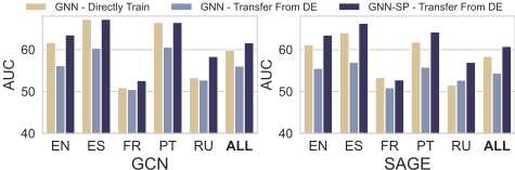
One-to-Multi Transfer. We use Twitch as the benchmark, which consists of six graphs with different sizes and data distributions. We pre-train the model on DE and fine-tune on other graphs (EN, ES, FR, PT, RU). We employ ROC-AUC as metric and adopt 2-layer GCN and SAGE as backbones. Figure 3 shows GNN-SP outperforms standard GNN with up to 8% improvements on ROC-AUC under FT Last Layer setting and achieves better performance than the model directly trained on the target over 10 out of 12 settings. The results validate the generalizability of GNN-SP to multiple graphs.
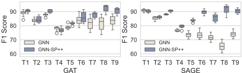
TransferwithDynamic Shift. In this scenario, we evaluate the model's capability to handle temporal distribution shifts. We first adopt a dynamic financial network Elliptic with splitting 5/5/33 snapshots for train/valid/test. Figure 4 presents the results where the test snapshots are grouped into 9 folds. The performance gain of our GNN-SP is up to 10% and 24% over GAT and SAGE, respectively. Additionally, we use Arxiv as another temporal dataset, where nodes represent papers published from 2005 to 2020 and edges indicate citations. Based on the publication time, we collect five sub-graphs, represented as Time 1 (2005 - 2007), Time 2 (2008 - 2010), Time 3 (2011 - 2014), Time 4 (2015 - 2017), and Time 5 (2018 - 2020). We use the first four graphs as sources and the last one as the target. The results are presented in Table 4 where our GNN-SP++ achieves significant improvements over all baselines.
4.3 Ablation Study
Transfer without Fine-tuning. Following [Liu et al., 2023a], we take a further step by directly employing the pretrained model on target graph without fine-tuning. Table 6 presents the transfer learning performance on Citation and Arxiv. We also adopt another domain adaptation setting (Degree) from [Gui et al., 2022]. It is obvious that our The reported results are from [Liu et al., 2023a]. ∗ indicates the results of our implementations based on the official code.
| ACM→DBLP | DBLP→ACM | Twitch-All | Arxiv-T1 | Arxiv-T3 | |
|---|---|---|---|---|---|
| GCN + Fully FT | 97.75 ± 0.16 | 80.03 ± 0.22 | 60.59 ± 1.13 | 69.29 ± 0.16 | 69.70 ± 0.39 |
| GCN-SP + FT Last Layer | 98.20 ± 0.54 | 79.20 ± 0.73 | 61.66 ± 0.92 | 71.43 ± 0.52 | 74.04 ± 0.83 |
| GCN-SP + Fully FT | 98.66 ± 0.29 | 80.82 ± 0.59 | 61.77 ± 0.98 | 73.12 ± 0.93 | 75.01 ± 0.62 |
| ACM & DBLP | Arxiv | |||
|---|---|---|---|---|
| Model | A → D | D → A | Time 1 | Degree |
| GCN∗ | 59.02 ± 1.04 | 59.20 ± 0.70 | 28.08 ± 0.24 | 57.41 ± 0.14 |
| GAT∗ | 61.67 ± 3.54 | 62.18 ± 7.04 | 32.32 ± 1.10 | 58.10 ± 0.15 |
| DANN | 59.02 ± 7.79 | 65.77 ± 0.46 | 24.33 ± 1.19 | 56.13 ± 0.18 |
| CDAN | 60.56 ± 4.38 | 64.35 ± 0.83 | 25.85 ± 1.15 | 56.43 ± 0.45 |
| UDAGCN | 59.62 ± 2.86 | 64.74 ± 2.51 | 25.64 ± 3.04 | 55.77 ± 0.83 |
| EERM | 40.88 ± 5.10 | 51.71 ± 5.07 | - | - |
| MIXUP | 49.93 ± 0.89 | 63.36 ± 0.66 | 28.04 ± 0.18 | 59.22 ± 0.22 |
| EGI∗ | 49.03 ± 1.50 | 64.40 ± 1.03 | 25.59 ± 0.25 | 56.93 ± 0.23 |
| SR-GNN∗ | 62.49 ± 1.96 | 63.32 ± 1.49 | 25.44 ± 0.30 | 56.98 ± 0.12 |
| GRADE∗ | 67.29 ± 2.04 | 64.13 ± 3.12 | 25.69 ± 0.12 | 57.49 ± 0.39 |
| SSReg∗ | 69.04 ± 2.95 | 65.93 ± 1.05 | 27.93 ± 0.29 | 56.67 ± 0.33 |
| StruRW | 70.19 ± 2.10 | 65.07 ± 1.98 | 28.46 ± 0.18 | 57.45 ± 0.15 |
| GCN-SP++ | 75.88 ± 5.57 | 71.32 ± 1.33 | 40.41 ± 1.07 | 64.35 ± 0.41 |
| GAT-SP++ | 73.78 ± 8.13 | 67.05 ± 4.97 | 36.38 ± 2.50 | 65.53 ± 0.60 |
Table 6: Node classification results without fine-tuning.
proposed SP layer significantly improves the transfer learning performance by enhancing the quality of the encoder.
Transfer with Fully Fine-tuning. We present transfer learning performance by fine-tuning the whole model in Table 5. We observe even if GNN-SP only fine-tunes the last layer, it still outperforms standard GNN with full fine-tuning. If our GNN-SP is fully fine-tuned, the model performance can be further improved, especially on large-scaled Arxiv.
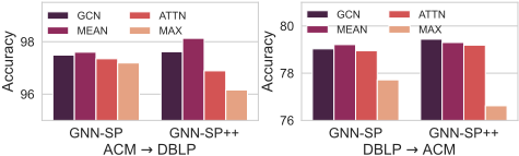
Pooling Methods. We evaluate model performance with different pooling functions, including MEAN, ATTN, MAX, and GCN. Figure 5 presents the experimental results over Citation network with GCN backbone. We observe the basic MEAN pooling outperforms complicated GCN and ATTN that adaptively determine the pooling weights wij. It is might because the complicated methods introduce extra inductive bias with unexpected noises.
5 RelatedWorks
Existing studies are typically categorized based on the availability of the target graph during the pre-training phase.
Pre-training with Target Graph. Researchers developed methods to explicitly align source and target graphs during pre-training, ensuring PS(Z) = PT (Z). For example, [Zhang et al., 2019; Dai et al., 2022b] adopt adversarial learning [Ganin et al., 2016] to train domain-invariant encoder, and following UDAGCN [Wu et al., 2020] incorporates attention to further enhance expressiveness. Alternatively, one can employ regularizers [Zhu et al., 2021a; Zhu et al., 2023; Shi et al., 2023], such as MMD and CMD, to constrain the discrepancy between the source and target. To facilitate this process, new graph-specific discrepancy metrics are proposed, including tree mover distance [Chuang and Jegelka, 2022], subtree discrepancy [Wu et al., 2023a], and spectral regularizer [You et al., 2023]. Additionally, [Liu et al., 2023a] emphasizes the most relevant instances in the source to better match distributions of the source and target. While these methods effectively reduce the distribution shift between source and target, the target graph may be unavailable during pre-training in many real-world scenarios.
Pre-training without Target Graph. Existing works aim to train GNNs transferable to unseen graphs. For example, EERM [Wu et al., 2022b] and following works [Chen et al., 2022; Wu et al., 2022c; Wu et al., 2023b; Yu et al., 2023] utilize causal learning to develop environment-invariant encoder. GTrans [Jin et al., 2023] transforms the target graph at test-time to align the source and target. Moreover, various studies employ augmentation to enhance the robustness of encoder against permutations [Verma et al., 2021; Wang et al., 2021; Liu et al., 2022; Han et al., 2022; Liu et al., 2023b; Guo et al., 2023] or apply disentangle learning to extract domain-invariant semantics [Ma et al., 2019; Liu et al., 2020]. To understand the transferability of GNNs, [Ruiz et al., 2020; Levie et al., 2021; Cao et al., 2023] interpret graphs as the combination of graphons, while [Han et al., 2021; Zhu et al., 2021b; Sun et al., 2023; Qiu et al., 2020] adopt self-supervised learning to identify transferable structures. Despite these efforts to enhance transferability, they cannot well address the negative transfer issue. To this end, we systematically analyze why the negative transfer happens and provide insights to solve this issue.
6 Conclusion
In this paper, we analyze the negative transfer in GNNs and introduce Subgraph Pooling, a simple yet effective method, to mitigate the issue. Our method transfers the subgraph-level knowledge to reduce the discrepancy between the source and target graphs, and is applicable for any GNN backbone without introducing extra parameters. We provide a theoretical analysis to demonstrate how the model works and conduct extensive experiments to evaluate its superiority under various transfer learning settings.
Acknowledgements
This work was partially supported by the NSF under grants IIS-2321504, IIS-2334193, IIS-2340346, IIS-2203262, IIS2217239, CNS-2203261, and CMMI-2146076. Any opinions, findings, and conclusions or recommendations expressed in this material are those of the authors and do not necessarily reflect the views of the sponsors.
@inproceedings{ijcai2024p570,
  title     = {Subgraph Pooling: Tackling Negative Transfer on Graphs},
  author    = {Wang, Zehong and Zhang, Zheyuan and Zhang, Chuxu and Ye, Yanfang},
  booktitle = {Proceedings of the Thirty-Third International Joint Conference on
               Artificial Intelligence, {IJCAI-24}},
  publisher = {International Joint Conferences on Artificial Intelligence Organization},
  editor    = {Kate Larson},
  pages     = {5153--5161},
  year      = {2024},
  month     = {8},
  note      = {Main Track},
  doi       = {10.24963/ijcai.2024/570},
  url       = {https://doi.org/10.24963/ijcai.2024/570},
}
TY - CPAPER TI - Subgraph Pooling: Tackling Negative Transfer on Graphs AU - Wang, Zehong AU - Zhang, Zheyuan AU - Zhang, Chuxu AU - Ye, Yanfang T2 - Proceedings of the Thirty-Third International Joint Conference on Artificial Intelligence, IJCAI-24 PB - International Joint Conferences on Artificial Intelligence Organization PY - 2024 SP - 5153 EP - 5161 DO - 10.24963/ijcai.2024/570 UR - https://doi.org/10.24963/ijcai.2024/570 ER -Copied
Machine-readable versions of this paper, for tools and AI agents:





