
Attribution Quality Metrics with Magnitude Alignment
Proceedings of the Thirty-Third International Joint Conference on Artificial Intelligence. Main Track. Pages 530-538.
https://doi.org/10.24963/ijcai.2024/59
Keywords
- Machine Learning: ML: Explainable/Interpretable machine learning
- AI Ethics, Trust, Fairness: ETF: Explainability and interpretability
- Computer Vision: CV: Interpretability and transparency
- AI Ethics, Trust, Fairness: ETF: Trustworthy AI
Abstract
Attribution algorithms play an instrumental role in human interpretation of AI models. The methods measure the importance of the input features to the model output decision, which can be displayed as an attribution map for image classifiers. Perturbation tests are the state-of-the-art approach to evaluate the quality of an attribution map. Unfortunately, we observe that perturbation tests fail to consider attribution magnitude, which translates into inconsistent quality scores. In this paper, we propose Magnitude Aligned Scoring (MAS), a new attribution quality metric that measures the alignment between the magnitude of the attributions and the model response. In particular, the metric accounts for both the relative ordering and the magnitude of the pixels within an attribution. In the experimental evaluation, we compare the MAS metric with existing metrics across a wide range of models, datasets, attributions, and evaluations. The results demonstrate that the MAS metric is 4x more sensitive to attribution changes, 2x more consistent, and 1.6x more invariant to baseline modifications. Our code and the referenced appendix are publicly available via https://github.com/chasewalker26/Magnitude-Aligned-Scoring.
- [Adebayo et al., 2018] Julius Adebayo, Justin Gilmer, Michael Muelly, Ian Goodfellow, Moritz Hardt, and Been Kim. Sanity checks for saliency maps. NeurIPS, 31, 2018.
- [Ancona et al., 2018] Marco Ancona, Enea Ceolini, Cengiz Öztireli, and Markus Gross. Towards better understand- ing of gradient-based attribution methods for deep neural networks. In International Conference on Learning Rep- resentations, 2018.
- [Borji et al., 2013] Ali Borji, Dicky N. Sihite, and Laurent Itti. Quantitative analysis of human-model agreement in visual saliency modeling: A comparative study. IEEE Transactions on Image Processing, 22(1):55-69, 2013.
- [Bylinskii et al., 2019] Zoya Bylinskii, Tilke Judd, Aude Oliva, Antonio Torralba, and Frédo Durand. What do dif- ferent evaluation metrics tell us about saliency models? IEEE Transactions on Pattern Analysis and Machine In- telligence, 41(3):740-757, 2019.
- [Chefer et al., 2021] Hila Chefer, Shir Gur, and Lior Wolf. Transformer interpretability beyond attention visualiza- tion. In Proceedings of the IEEE/CVF conference on computer vision and pattern recognition, pages 782-791, 2021.
- [Cheng et al., 2017] Gong Cheng, Junwei Han, and Xiao- qiang Lu. Remote sensing image scene classification: Benchmark and state of the art. Proceedings of the IEEE, 105(10):1865-1883, 2017.
- [Das and Rad, 2020] Arun Das and Paul Rad. Opportunities and challenges in explainable artificial intelligence (xai): A survey, 2020.
- [Dosovitskiy et al., 2020] Alexey Dosovitskiy, Lucas Beyer, Alexander Kolesnikov, Dirk Weissenborn, Xiaohua Zhai, Thomas Unterthiner, Mostafa Dehghani, Matthias Min- derer, Georg Heigold, Sylvain Gelly, et al. An image is worth 16x16 words: Transformers for image recognition at scale. arXiv preprint arXiv:2010.11929, 2020.
- [Hao et al., 2021] Yaru Hao, Li Dong, Furu Wei, and Ke Xu. Self-attention attribution: Interpreting information inter- actions inside transformer. In Proceedings of the AAAI Conference on Artificial Intelligence, volume 35, pages 12963-12971, 2021.
- [He et al., 2016] Kaiming He, Xiangyu Zhang, Shaoqing Ren, and Jian Sun. Deep residual learning for image recog- nition. In Proceedings of the IEEE conference on computer vision and pattern recognition, pages 770-778, 2016.
- [Hooker et al., 2019a] Sara Hooker, Dumitru Erhan, Pieter- Jan Kindermans, and Been Kim. A benchmark for inter- pretability methods in deep neural networks. Advances in neural information processing systems, 32, 2019.
- [Hooker et al., 2019b] Sara Hooker, Dumitru Erhan, Pieter- Jan Kindermans, and Been Kim. A benchmark for inter- pretability methods in deep neural networks. Advances in neural information processing systems, 32, 2019.
- [Kapishnikov et al., 2019] Andrei Kapishnikov, Tolga Bolukbasi, Fernanda Viegas, and Michael Terry. Xrai: Better attributions through regions. In 2019 IEEE/CVF International Conference on Computer Vision (ICCV), pages 4947-4956, Los Alamitos, CA, USA, nov 2019. IEEE Computer Society.
- [Kapishnikov et al., 2021a] Andrei Kapishnikov, Tolga Bolukbasi, Fernanda Viegas, and Michael Terry. Xrai code repository, 2021. Accessed: 2022-10-15.
- [Kapishnikov et al., 2021b] Andrei Kapishnikov, Subhashini Venugopalan, Besim Avci, Ben Wedin, Michael Terry, and Tolga Bolukbasi. Guided integrated gradients: an adap- tive path method for removing noise. In 2021 IEEE/CVF Conference on Computer Vision and Pattern Recognition (CVPR), pages 5048-5056, Los Alamitos, CA, USA, jun 2021. IEEE Computer Society.
- [Krippendorff, 2004] Klaus Krippendorff. Content Analysis: An Introduction to Its Methodology (second edition). Sage Publications, 2004.
- [Kümmerer et al., 2014] Matthias Kümmerer, Thomas Wal- lis, and Matthias Bethge. How close are we to un- derstanding image-based saliency? arXiv preprint arXiv:1409.7686, 2014.
- [Miglani et al., 2020] Vivek Miglani, Narine Kokhlikyan, Bilal Alsallakh, Miguel Martin, and Orion Reblitz- Richardson. Investigating saturation effects in integrated gradients, 2020.
- [Pan et al., 2021] Deng Pan, Xin Li, and Dongxiao Zhu. Ex- plaining deep neural network models with adversarial gra- dient integration. In Zhi-Hua Zhou, editor, Proceedings of the Thirtieth International Joint Conference on Arti- ficial Intelligence, IJCAI-21, pages 2876-2883. Interna- tional Joint Conferences on Artificial Intelligence Orga- nization, 8 2021. Main Track. IJCAI
- [Paszke et al., 2019] Adam Paszke, Sam Gross, Francisco Massa, Adam Lerer, James Bradbury, Gregory Chanan, Trevor Killeen, Zeming Lin, Natalia Gimelshein, Luca Antiga, Alban Desmaison, Andreas Köpf, Edward Yang, Zach DeVito, Martin Raison, Alykhan Tejani, Sasank Chilamkurthy, Benoit Steiner, Lu Fang, Junjie Bai, and Soumith Chintala. Pytorch: An imperative style, high- performance deep learning library. In Proceedings of the 33rd International Conference on Neural Information Pro- cessing Systems.
- [Petsiuk et al., 2018a] Vitali Petsiuk, Abir Das, and Kate Saenko. Rise code repository, 2018. Accessed: 2022-11- 01.
- [Petsiuk et al., 2018b] Vitali Petsiuk, Abir Das, and Kate Saenko. Rise: Randomized input sampling for explana- tion of black-box models. In Proceedings of the British Machine Vision Conference (BMVC), 2018.
- [Qiang et al., 2022] Yao Qiang, Deng Pan, Chengyin Li, Xin Li, Rhongho Jang, and Dongxiao Zhu. Attcat: Explain- ing transformers via attentive class activation tokens. In S. Koyejo, S. Mohamed, A. Agarwal, D. Belgrave, K. Cho, and A. Oh, editors, Advances in Neural Information Pro- cessing Systems, volume 35, pages 5052-5064.
- [Ribeiro et al., 2016] Marco Tulio Ribeiro, Sameer Singh, and Carlos Guestrin. "why should i trust you?" explain- ing the predictions of any classifier. In Proceedings of the 22nd ACM SIGKDD international conference on knowl- edge discovery and data mining, pages 1135-1144, 2016.
- [Russakovsky et al., 2015] Olga Russakovsky, Jia Deng, Hao Su, Jonathan Krause, Sanjeev Satheesh, Sean Ma, Zhiheng Huang, Andrej Karpathy, Aditya Khosla, Michael Bernstein, Alexander C. Berg, and Li Fei-Fei. Ima- geNet Large Scale Visual Recognition Challenge. Inter- national Journal of Computer Vision (IJCV), 115(3):211- 252, 2015.
- [Samek et al., 2016] Wojciech Samek, Alexander Binder, Grégoire Montavon, Sebastian Lapuschkin, and Klaus- Robert Müller. Evaluating the visualization of what a deep neural network has learned. IEEE transactions on neural networks and learning systems, 28(11):2660-2673, 2016.
- [Selvaraju et al., 2017] Ramprasaath R Selvaraju, Michael Cogswell, Abhishek Das, Ramakrishna Vedantam, Devi Parikh, and Dhruv Batra. Grad-cam: Visual explanations from deep networks via gradient-based localization. In Proceedings of the IEEE international conference on com- puter vision, pages 618-626, 2017.
- [Shrikumar et al., 2016] Avanti Shrikumar, Peyton Green- side, Anna Shcherbina, and Anshul Kundaje. Not just a black box: Learning important features through propagating activation differences. arXiv preprint arXiv:1605.01713, 2016.
- [Simonyan et al., 2014] Karen Simonyan, Andrea Vedaldi, and Andrew Zisserman. Deep inside convolutional networks: Visualising image classification models and saliency maps, 2014.
- [Springenberg et al., 2015] Jost Tobias Springenberg, Alexey Dosovitskiy, Thomas Brox, and Martin Ried- miller. Striving for simplicity: The all convolutional net, 2015.
- [Sundararajan et al., 2017] Mukund Sundararajan, Ankur Taly, and Qiqi Yan. Axiomatic attribution for deep net- works. In Proceedings of the 34th International Confer- ence on Machine Learning -Volume 70, ICML'17, page 3319-3328. JMLR.org, 2017.
- [Tomsett et al., 2020] Richard Tomsett, Dan Harborne, Supriyo Chakraborty, Prudhvi Gurram, and Alun Preece. Sanity checks for saliency metrics. In AAAI, volume 34, pages 6021-6029, 2020.
- [Yuan et al., 2021] Tingyi Yuan, Xuhong Li, Haoyi Xiong, Hui Cao, and Dejing Dou. Explaining information flow inside vision transformers using markov chain. In eXplain- able AI approaches for debugging and diagnosis., 2021.
- [Zeiler and Fergus, 2014] Matthew D Zeiler and Rob Fergus. Visualizing and understanding convolutional networks. In European conference on computer vision, pages 818-833. Springer, 2014.
References were extracted automatically from the PDF and may contain errors.
Full text extracted automatically from the PDF; figures, tables and equations may differ. The PDF is the version of record.
1 Introduction
Understanding the decision making of black-box AI models is necessary for deployment in safety-critical domains. Attribution methods are currently the most prevalent form of explanations [Das and Rad, 2020]. These methods provide model explanations by assigning an importance value to each feature of the model input [Simonyan et al., 2014]. A broad range of attribution algorithms have been developed in the past few years [Hooker et al., 2019a; Chefer et al., 2021]. However, the ability to quantify the quality of an attribution map remains an open problem. An accurate attribution metric has the potential to further advance the field of explainable AI forward, refining human understanding of AI models.
Attribution quality metrics generally fall into two categories: evaluation with ground-truth [Borji et al., 2013] or perturbation metrics without ground-truth [Samek et al.,
2016; Ancona et al., 2018]. Evaluation of attribution methods with ground-truth can be desirable when human-labeled data is present. Common methods to develop ground-truth datasets in the vision domain are the use of segmentation algorithms to create a mask of the image subject, human eyetracking heat map data, or manual image masks created by humans [K¨ummerer et al., 2014; Bylinskii et al., 2019]. Perturbation metrics aim to quantify the quality of an attribution map without the use of ground-truths that are often not available [Samek et al., 2016]. Moreover, human-created masks do not necessarily represent a model's decision process.
Perturbation metrics aim to evaluate if the attribution map is reflective of a model's decision making [Petsiuk et al., 2018b]. Specifically, perturbation tests aim to measure if the attribution map discriminates appropriately between more and less important features. The tests are performed by modifying the model or the input test image by the values in the attribution map [Petsiuk et al., 2018b]. Ideally, the magnitude of the attribution assigned to each feature should be proportional to the model response. However, we observe that current image perturbation metrics do not measure this relationship, they only account for the relative ordering of the input features, not the magnitudes, leading to inconsistent scores.
In this paper, we propose a new perturbation metric for evaluating attribution quality without ground-truth called Magnitude Aligned Scoring (MAS). MAS employs an alignment penalty to measure the relationship between attribution magnitude and the response of the model output to the attribution. Our main contributions can be summarized as follows:
- We observe that existing quality metrics fail to consider attribution magnitude and only rely on attribution order, which leads to inconsistent quantification.
- We propose a quantitative, ground-truth-free perturbation metric, MAS. It provides a principled solution to the failures of existing methods by utilizing an alignment penalty to satisfy a new sensitivity property we define.
- Quantitative analysis proves MAS solves the failures of existing metrics, showing 2.5× improvements across sensitivity, consistency, and baseline invariance testing.
The paper is arranged as follows: related work is discussed in Section 2, the MAS metric is motivated in Section 3, the MAS metric is defined in Section 4, experimental evaluation is performed in Section 5, and the conclusion is in Section 6.
2 RelatedWork
In this section, we discuss the details of attribution methods, the existing metrics that quantify their accuracy, and how these metrics can be validated.
2.1 AttributionMethods
Attribution methods explain black-box models by measuring the importance of each feature in an input to the model response. Attribution methods can be occlusion based [Ribeiro et al., 2016; Zeiler and Fergus, 2014], gradient based [Simonyan et al., 2014], or attention based methods [Hao et al., 2021] for transformer models. Occlusion based methods iteratively modify an input image while measuring model output to determine the most salient regions. Gradient based methods use backpropagation to measure the model gradients with respect to the input features. Attention based methods use transformer attention weights as explanations directly, or combine them with model gradients [Yuan et al., 2021]. Occlusion based methods are slow and generally undesirable.
The early gradient based techniques utilize model gradients as is [Simonyan et al., 2014] or multiply them by the input image [Shrikumar et al., 2016], but these methods suffer from large amounts of saturation noise [Sundararajan et al., 2017]. Recently, the newly introduced path integration methods [Miglani et al., 2020] average the gradients from multiple interpolated images along a path from a baseline to the input image to reduce this saturation noise. Additional techniques to reduce noise suppress negative gradients during the backpropagation step [Springenberg et al., 2015] or measure gradients from a models' last convolutional layer and remove gradients pointing to non-target classes [Selvaraju et al., 2017]. Attention based methods first started with raw attention as a visualization [Hao et al., 2021] and have since incorporated accumulation techniques [Yuan et al., 2021; Chefer et al., 2021] and gradients [Qiang et al., 2022] to create stronger attributions. Attribution metrics are necessary to measure how well an attribution represents a model.
2.2 Attribution QualityMetrics
Attribution quality metrics aim to evaluate how well an attribution represents a model's decision making process. We focus on improving perturbation metrics because ground-truths are generally not available. Within perturbation metrics, there are methods that perturb [Adebayo et al., 2018] or retrain a model [Hooker et al., 2019b] and those that perturb the input and retain the original model [Petsiuk et al., 2018b]. These model modification metrics either randomize model layers and measure how much an attribution changes [Adebayo et al., 2018], or retrain a model with the top attribution pixels ablated from the train set [Hooker et al., 2019b]. Since these methods require data intensive and model-specific retraining or modification, we will focus on image perturbation metrics for this work [Petsiuk et al., 2018b].
Image perturbation metrics exist as insertion or deletion tests and use the original image, an attribution, a baseline (blurred starting image for insertion or black ending image for deletion), and the model. In insertion (deletion) testing, original (black) pixels are iteratively added to the blurred (original) input image in order of descending attribution magnitude until the original (a black) image is reached. The model output is measured for the perturbed image at each iteration with respect to the original class, resulting in a receiver operating characteristics (ROC) curve. For insertion (deletion) tests, this is an increasing (decreasing) curve and the area under the ROC curve - the AUC - gives the final result, where a higher (lower) value represents a better attribution. This traditional ROC curve is visualized in Figure 2(b) for the insertion test. It is most common for the results of both the insertion and deletion tests to be presented for the evaluation of an attribution. In this work we evaluate two methods which follow this perturbation process.
RISE: Insertion and Deletion. In the RISE paper [Petsiuk et al., 2018b], the authors use the standard baselines for the insertion and deletion tests (the blurred input or black image), and use equally sized pixel groupings during the testing process. At each perturbation step, they select the top N pixels of an N ×N image by descending attribution magnitude and measure the resulting softmax output to generate an ROC.
PIC: SIC and AIC Insertion. Kapishnikov et al. present the performance information curve (PIC) insertion metrics: the softmax information curve (SIC) and accuracy information curve (AIC) scores [Kapishnikov et al., 2019]. SIC uses the softmax output, whereas AIC uses an accuracy measurement of 0 or 1 for an incorrect or correct prediction at each perturbation step. Instead of a uniform blur baseline, the input image is blurred in discrete, polygonal tiles, with unique noise distributions. Additionally, pixels are non-linearly perturbed in groups of increasing size, and the SIC/AIC ROCs are normalized to be monotonic non-decreasing curves.
2.3 Desirable AttributionMetric Properties
A trustworthy and reliable attribution quality metric should adhere to the following desirable properties which are quantitatively measurable:
- Sensitivity: Features important to the model should have high attribution and unimportant features should have low attribution [Petsiuk et al., 2018b].
- Consistency: A metric should be consistent in its calculated ratings. It should consistently rank different attribution methods by their quality over a set of varying inputs [Tomsett et al., 2020].
- Baseline Invariance: Ametric should be invariant to its baseline selection, i.e., an insertion test using a random baseline or blurred baseline should rank a set of attributions the same way [Tomsett et al., 2020].
Existing image perturbation metrics attempt to satisfy sensitivity by scoring attributions using the relative ordering of the input features. However, the sensitivity property is rather vaguely defined, so it is not clear which one of the RISE and PIC metrics best quantifies the property. Hence, a mix of the different tests are typically used to evaluate new attribution algorithms. Additionally, it has been shown that consistency and baseline invariance are not adequately satisfied by the RISE and PIC methods [Tomsett et al., 2020].
3 Motivating a NewMetric
We now study the RISE and PIC metrics to show their failure of sensitivity resulting from their disregard of attribution magnitude and motivate the definition of a new sensitivity property as well as the development of a new metric.
3.1 AttributionMagnitude Is Important
In Section 2.3, the sensitivity property states that input pixels that are important (not important) to the model's decision should be assigned large (small) magnitude attributions. Here, small and large refers to the relative distance to zero. Formally, let Ai and Aj denote the attributions of pixels i and j, respectively. The quotient Ai/Aj measures the relationship of the features' magnitudes, which defines sensitivity.
Given this notation, we analyze the invariance of attribution metrics to multiplying an attribution map by a constant or adding a constant. It is straightforward to understand that invariance to multiplication is desirable for a metric, as Ai/Aj is equal to aAi/aAj, where a is a constant. However, (Ai +a)/(Aj +a) is not equal to Ai/Aj, in general. Therefore, invariance to a constant offset is undesirable under the sensitivity property, but existing metrics do not adhere to this.
3.2 Limitations of State of the Art Metrics
Increase by a Constant Is Ignored
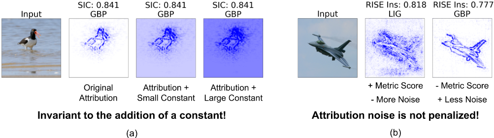
In Figure 1(a), we modify guided backpropagation (GBP) [Springenberg et al., 2015] attributions by adding 5% or 10%×max(GBP) to all attribution pixels as a constant. Since adding a constant does not change the relative ordering of the input features, the attribution maps are scored equally by SIC. This holds for all four reviewed metrics - RISE insertion and deletion as well as PIC's SIC and AIC. Thus, it is clear the existing attribution metrics' sole reliance on relative attribution ordering leads to an invariance to a constant offset.
Theorem 1. RISE and PIC Are Invariant to Constant Offset.
Proof. Let an attribution A with values in the range [0, 1] have a magnitude ordering of OA. If a constant b is added to A, this yields A′ , with range [b, 1 + b] and ordering OA′ =
OA. Since a score is determined solely by the perturbation of the input image via the order of A, and OA = OA′ , A and A′ will have equal scores. Therefore, the metrics are invariant to a constant offset.
Attribution Noise Is Not Penalized
We show the attribution maps of a "warplane" image computed using left integrated gradients (LIG) [Miglani et al., 2020] and GBP in Figure 1(b). Although GBP has a very sharp, low noise attribution compared to LIG, which has evident saturation noise [Sundararajan et al., 2017], the RISE insertion metric scores LIG higher than GBP. Given the attributions are nearly identical except for the noise in LIG, it is clear that existing metrics do not sufficiently penalize nonzero attributions on unimportant input features. This is a direct result of not adhering to the sensitivity property.
3.3 Proportional Sensitivity
In this paper, we propose a quantitatively satisfiable property in replacement of the vaguely defined sensitivity property:
- Proportional Sensitivity: The magnitude of the attribution assigned to an input feature should be directly proportional to the change the feature induces in the model output response.
To satisfy this property, we propose a new metric that penalizes the misalignment of an attribution feature's model response and density response. This encourages large magnitude attributions to be assigned to the critical input features while penalizing non-zero attributions assigned to pixels that are irrelevant to the model. We envision this new metric will drive the development of new attribution algorithms that produce sharp, low noise attribution maps.
4 The MASMetric
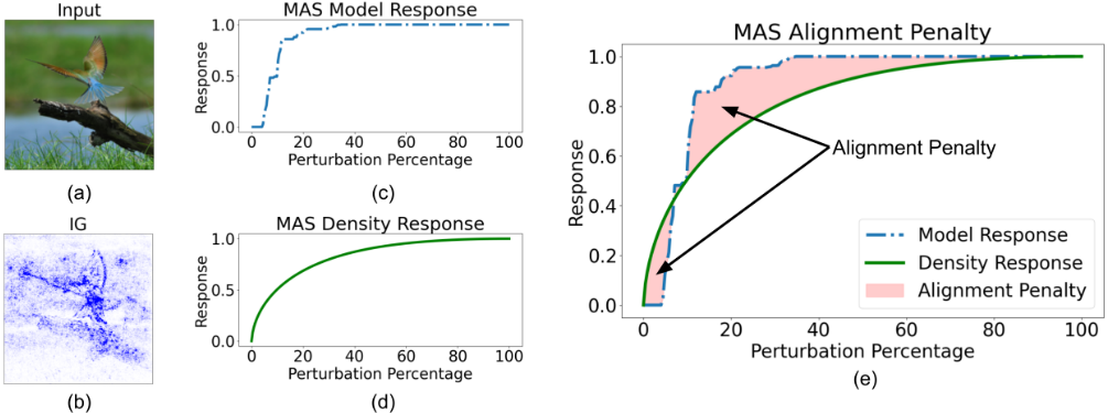
In this section, we introduce the magnitude aligned scoring (MAS) metric. We define the model and density response to introduce an alignment penalty that satisfies the proportional sensitivity property. The model response measures a feature's proportional contribution to the model output and the density response measures a feature's proportional contribution to the entire attribution's magnitude. Figure 2 provides an overview.
4.1 The Model and Density Response
Given an input X of class c, a model F, and an attribution map A, N attribution features are evaluated over an N step perturbation test. For a step k, the perturbed image Xk evaluates the impact of the first k attribution features in highest magnitude order. This test follows the RISE process from Section 2.2. We define the model response (MR) at step k as:
where X0 represents the unperturbed starting image and MR0 toMRN forms theMR curve. In Figure 2, we show an input image of a "bee eater" (a), its integrated gradients (IG) [Sundararajan et al., 2017] attribution map (b), and the model response (c) from an MAS insertion test. We note that the insertion model response MRins is a monotonically increasing curve, andMRdel is a monotonically decreasing curve.
Next, we define the density response (DR) at step k as:
where the |.| operation measures the total magnitude of the attributions in a given feature, A0 represents 0 selected features, and DR0 to DRN forms a full density response curve. The density response of the "bee eater" IG attribution is seen in Figure 2(d) and represents, at each step, what percentage of the total attribution magnitude has been selected via the perturbation process. We note that the insertion model response DRins is a monotonically increasing curve, and DRdel = 1 -DRins is a monotonically decreasing curve.
Now we define the alignment penalty (AP) which measures the absolute value of the difference between the model and density response for an attribution map. The general alignment penalty at step k is defined as:
where AP0 to APN measures the alignment penalty across the full insertion or deletion MR and DR curves. In Figure 2(e), the insertion alignment penalty is illustrated as the area between the MR and DR curves.
4.2 Magnitude Aligned Scoring (MAS)
Given an attribution map A with N features, MAS can be utilized as insertion or deletion. The insertion and deletion tests are defined by the AUC of the MR and AP curves:
and
Intuitively, lowering (increasing) the insertion (deletion) score is the effective application of the alignment penalty because a higher (lower) insertion (deletion) score represents a higher quality attribution.
To calculate the MR, we perform the linear perturbation process from RISE explained in Section 2.2 and we perform monotonic normalization of the MR to [0, 1] to ensure AP = 0 is achievable as DR is on the range [0, 1]. The penalized MASins or MASdel ROC is then clipped to the range [0, 1] and normalized to [0, 1]. Therefore, the AUC of the resulting MAS ins and MAS del scores is on the range [0, 1] where higher is better for MAS ins and lower for MAS del .
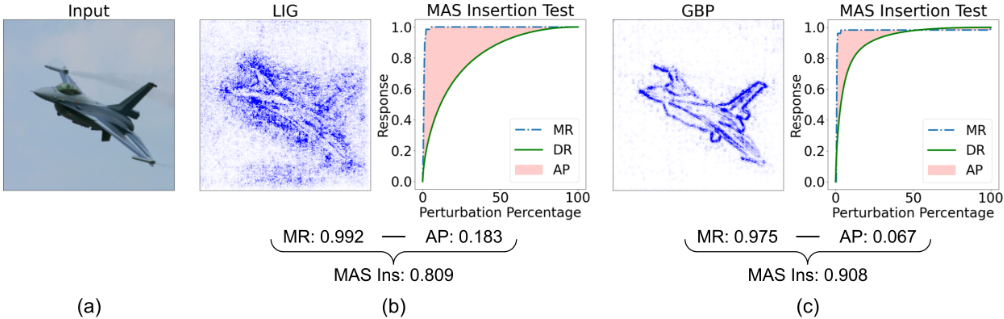
We present how the MAS insertion test accounts for attribution magnitude in Figure 3 by revisiting the LIG and GBP attributions of the "warplane" seen in Figure 1(b). From left to right, we show the input (a), an attribution, its MR, DR, and AP graph, and its MAS score calculation beneath. In Figure 3(b) we see LIG has a large model response of 0.992 which is greater than GBP's model response of 0.975 in Figure 3(c) (since magnitude is not a factor without the alignment penalty). However, due to the noise in the LIG attribution, it has a large alignment penalty of 0.183 compared to 0.067 for GBP. When the AP is subtracted from the MR of each attribution, the final scores are 0.809 and 0.908 for LIG and GBP, respectively. The proper penalization of noise in the LIG attribution results in a lower score than GBP, as expected.
Insertion and Deletion Difference. In the existing literature, insertion and deletion tests are often performed in unison, but considered separately as they measure different qualities of an attribution. The insertion test measures the value of high magnitude attributions to classification by adding them to an image, while the deletion test measures the value of high magnitude attributions to misclassification by removing them from an image. However, we propose a combination of the scores should also be considered to balance the bias of each test. We propose considering the difference of the scores:
The subtraction of these two tests creates the new "difference" score while preserving their opposing nature: higher insertion scores and lower deletion scores are desired. If one score measures very well and one very poorly, the small difference will indicate the disagreement between the tests (one test is biased). If both scores are respectively strong, the large difference will indicate an overall high scoring attribution.
4.3 MAS Is Sensitive to a Constant Offset
Theorem 2. MAS is sensitive to a constant offset.
Proof. The MAS score of an attribution A is defined as:
where MR is equivalent to the score of the RISE metrics. Following Proof (3.2), if MAS(A) and MAS(A′ ) are evaluated, the MR terms of each function will be equivalent.
So we write MAS = f(DR). Now, consider A ∈ [0, 1] and A′ ∈ [b, 1 + b]. By Eq (2), DR(A) ̸= DR(A′ ), thus MAS(A) ̸= MAS(A′ ), proving MAS is sensitive to a constant offset, satisfying proportional sensitivity.
5 Evaluation
We perform evaluation of the proposed MAS metrics against the currently accepted PIC [Kapishnikov et al., 2019] and RISE [Petsiuk et al., 2018b] perturbation metrics for a total of eight metrics under evaluation: AIC, SIC, RISE insertion, RISE deletion, RISE difference, MAS insertion, MAS deletion, and MAS difference. We recognize difference was not employed in the original RISE framework, but we use it for fair comparison against our proposed MAS difference metric.
All evaluations are performed with PyTorch [Paszke et al., 2019], using ResNet 101 (R101) [He et al., 2016] and ViTBase 16 (VIT16) [Dosovitskiy et al., 2020]. The evaluations are executed on an internal cluster with NVIDIA A40 GPUs. We employ the Imagenet [Russakovsky et al., 2015] and RESISC45 [Cheng et al., 2017] datasets across our experiments. We use the respective repositories of the PIC [Kapishnikov et al., 2021a] and RISE [Petsiuk et al., 2018a] metrics.
5.1 Metric Attribution Sensitivity Test
As presented in Figure 1(a) and (b), the RISE and PIC metrics do not recognize a constant offset or properly penalize attribution noise because they do not consider attribution magnitude, and therefore are not sensitive as outlined in Section 2.3. We now quantitatively verify MAS' sensitivity.
Using the ImageNet and RESISC45 datasets with the R101 and VIT16 models, we generate gradient (grad) [Simonyan et al., 2014], LIG, and GBP attributions for 1000 images from both datasets. We choose these attribution methods for their different levels of noise. We then perform one of two modifications to the generated attributions. We either add a constant that is 5, 10, 25, or 50% of the maximum attribution value as explained for Figure 1(a) or we add noise from the range 0 to 0.05, 1, 2, or 3% of the maximum attribution value.
| Noise Type | Constant Offset | Noised | ||||||
|---|---|---|---|---|---|---|---|---|
| Dataset | ImageNet | RESISC 45 | ImageNet | RESISC 45 | ||||
| Model | R101 | VIT16 | R101 | VIT16 | R101 | VIT16 | R101 | VIT16 |
| PIC: SIC [Kapishnikov et al., 2019] (↑) | 0.00 | 0.00 | 0.00 | 0.00 | 2.63 | 0.89 | 0.46 | 0.74 |
| PIC: AIC [Kapishnikov et al., 2019] (↑) | 0.00 | 0.00 | 0.00 | 0.00 | 2.80 | 0.88 | 0.74 | 0.55 |
| RISE Ins [Petsiuk et al., 2018b] (↑) | 0.00 | 0.00 | 0.00 | 0.00 | 14.17 | 3.43 | 1.51 | 3.77 |
| RISE Del [Petsiuk et al., 2018b] (↑) | 0.00 | 0.00 | 0.00 | 0.00 | 4.99 | 3.88 | 2.39 | 1.55 |
| RISE Diff [Petsiuk et al., 2018b] (↑) | 0.00 | 0.00 | 0.00 | 0.00 | 8.94 | 2.28 | 1.80 | 2.68 |
| MAS Ins (ours) (↑) | 20.41 | 20.21 | 25.08 | 27.51 | 14.65 | 9.84 | 11.60 | 18.16 |
| MAS Del (ours)(↑) | 23.39 | 21.10 | 25.43 | 27.10 | 12.18 | 4.00 | 12.92 | 14.02 |
| MAS Diff (ours) (↑) | 22.02 | 20.67 | 25.25 | 27.31 | 13.32 | 6.86 | 12.25 | 16.12 |
| Dataset | ImageNet | RESISC 45 | ||
|---|---|---|---|---|
| Model | R101 | VIT16 | R101 | VIT16 |
| PIC: SIC [Kapishnikov et al., 2019] (↑) | 0.323 | 0.262 | 0.025 | 0.268 |
| PIC: AIC [Kapishnikov et al., 2019] (↑) | 0.185 | 0.263 | 0.017 | 0.382 |
| RISE Ins [Petsiuk et al., 2018b] (↑) | 0.479 | 0.128 | 0.015 | 0.056 |
| RISE Del [Petsiuk et al., 2018b] (↑) | 0.378 | 0.330 | 0.181 | 0.117 |
| RISE Diff [Petsiuk et al., 2018b] (↑) | 0.657 | 0.448 | 0.071 | 0.162 |
| MAS Ins (ours) (↑) | 0.634 | 0.491 | 0.158 | 0.259 |
| MAS Del (ours) (↑) | 0.678 | 0.669 | 0.497 | 0.500 |
| MAS Diff (ours) (↑) | 0.715 | 0.650 | 0.237 | 0.387 |
We then average, over the images, the ROCs computed by each of the eight metrics for all attributions and their modifications. We then measure the absolute distance of the modified attribution ROCs from the original ROC. We evaluate a metric's sensitivity by the ratio of the distance metric to the original attribution's AUC. A sensitive metric will have a non-zero ratio value, where higher indicates more sensitivity.
In Table 1, we see only MAS is sensitive to a constant offset and MAS outperforms PIC and RISE in all noised sensitivity tests. MAS is overall more sensitive to changes in an attribution as it considers attribution magnitude via the alignment penalty. In Section A.1, we present the ROC curves from the table that showMAS reduces the score of the modified (worse) attributions, whereas PIC and RISE do not consistently increase or decrease the score if the score changes.
5.2 Metric Ranking Consistency Test
To evaluate the consistency of how a metric rates a group of attributions, we perform two metric sanity checks [Tomsett et al., 2020]: inter-rater reliability (IRR) and internal consistency reliability (ICR). IRR measures how well a metric sorts a set of attributions over a set of images. A perfectly consistent metric is expected to provide the same ordering of an attribution set over all images. Krippendorff's α is used to measure the IRR of a metric [Krippendorff, 2004], where a higher α in the range [0, 1] represents a more consistent metric. We provide the ICR results in Appendix A.2.
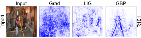
We measure the IRR of the eight metrics using three attributions over 5000 images from the ImageNet and RESISC45 datasets. For the R101 model, we select the grad, LIG, and GBP attributions due to their large visual differences (see Figure 4). For the VIT16 model, we select the following attribution group: a random mask, LIG, and transition attention [Yuan et al., 2021] or raw attention [Hao et al., 2021] for ImageNet and RESISC45, respectively, due to their large visual differences. These were chosen as visually similar attributions are likely to be scored equivalently, making consistent ranking unlikely for any metric. The IRR test results are in Table 2 where MAS shows a significantly higher consistency than the RISE and PIC metrics, outperforming them in 11/12 tests. We illustrate the consistency improvements of MAS with Figure 5 and figures in Appendix A.2.
| Baseline | Random | Dataset Mean | ||||||
|---|---|---|---|---|---|---|---|---|
| Dataset | ImageNet | RESISC 45 | ImageNet | RESISC 45 | ||||
| Model | R101 | VIT16 | R101 | VIT16 | R101 | VIT16 | R101 | VIT16 |
| RISE Ins [Petsiuk et al., 2018b] (↑) | 0.495 | 0.331 | 0.056 | 0.177 | 0.505 | 0.312 | 0.052 | 0.174 |
| RISE Del [Petsiuk et al., 2018b] (↑) | 0.369 | 0.235 | 0.131 | 0.052 | 0.368 | 0.247 | 0.157 | 0.045 |
| RISE Diff [Petsiuk et al., 2018b] (↑) | 0.600 | 0.537 | 0.131 | 0.267 | 0.610 | 0.550 | 0.149 | 0.265 |
| MAS Ins (ours) (↑) | 0.554 | 0.463 | 0.160 | 0.287 | 0.554 | 0.463 | 0.166 | 0.283 |
| MAS Del (ours) (↑) | 0.680 | 0.631 | 0.466 | 0.496 | 0.680 | 0.631 | 0.490 | 0.477 |
| MAS Diff (ours) (↑) | 0.660 | 0.606 | 0.296 | 0.430 | 0.674 | 0.606 | 0.319 | 0.419 |
5.3 Metric Baseline Invariance Test
As explained in Section 2.3, it is desirable for a quality metric to consistently evaluate attributions regardless of its baseline. ICR measures how well two different metrics agree on attribution rankings via Spearman's ρ ∈ [0, 1], where a higher value represents stronger agreement. We evaluate the agreement of the six RISE and MAS quality metrics with their modified baseline versions. We exclude PIC due to inaccessibility of modification. We use either random values drawn from a uniform distribution or the dataset mean value as the new baseline [Tomsett et al., 2020]. The default baseline for insertion is a blurred image and for deletion, a black image. We use the same image, model, and attribution choices from the previous section for evaluation. The results in Table 3 show that MAS is more invariant to baseline modification than RISE in 24/24 tests, as desired. A visual explanation of this test is provided with a figure in Appendix A.3.
5.4 Qualitative Analysis of MAS
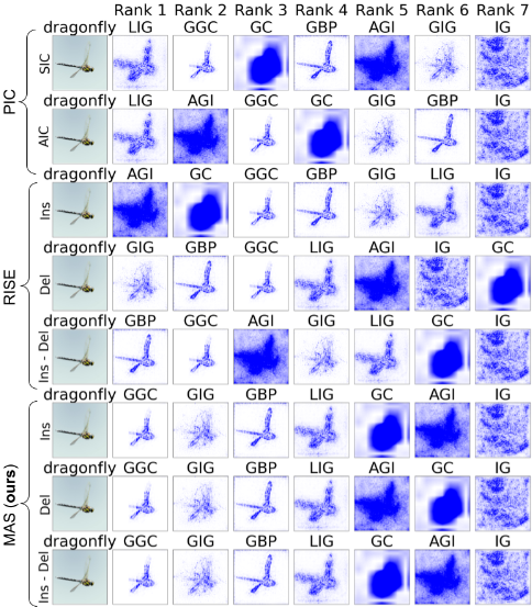
To qualitatively verify MAS against PIC and RISE, we provide ten examples in Appendix A.4 and one in Figure 5. We score seven attributions: IG, LIG, GBP, GradCAM and guided GradCAM [Selvaraju et al., 2017], guided IG (GIG) [Kapishnikov et al., 2021b], and adversarial gradient integration (AGI) [Pan et al., 2021] using the eight tests discussed in this paper. This figure evaluates the properties of sensitivity and consistency. Observing the location of noisy attributions in the orderings, MAS shows greatly improved sensitivity by placing noisy attributions at the worst ranks across all three metrics, whereas RISE and PIC fail to do so. The figure also shows that the RISE and PIC tests do not sort consistently compared to MAS which is consistent in ranks 1 - 4 and 7.
6 Conclusion
We discover that current state-of-the-art attribution quality metrics fail to consider attribution magnitude which leads to poor quantification as they fail invariance properties.
Through the introduction of the alignment penalty to account for the relationship between attribution magnitude and model response, we define the MAS framework which properly evaluates attributions. We show quantitatively that the MAS metrics, unlike the existing state-of-the-art metrics, satisfy the three desired properties of attribution quality metrics: sensitivity, consistency, and invariance to baseline selection. This greatly improves the ability of a user to select a desired, high-performance attribution method. We believe MAS will be used to develop high-quality attribution methods. In future work, we intend to use the alignment penalty to refine existing attributions by removing unimportant features.
Acknowledgements
The authors were in part supported by Lockheed Martin Corporation and the Florida High Tech Corridor. This material is partially based on research sponsored by DARPA under agreement number #FA8750-23-2-0501 and #HR00112020002. This material is partially based upon work supported by the U.S. Department of Energy, Office of Science, Office of Advanced Scientific Computing Research, under Award Number #DE-SC0023494. The U.S. Government is authorized to reproduce and distribute reprints for Governmental purposes notwithstanding any copyright notation thereon. The views and conclusions contained herein are those of the authors and should not be interpreted as necessarily representing the official policies or endorsements, either expressed or implied, of DARPA, or DOE, or the U.S. Government.
@inproceedings{ijcai2024p59,
  title     = {Attribution Quality Metrics with Magnitude Alignment},
  author    = {Walker, Chase and Simon, Dominic and Chen, Kenny and Ewetz, Rickard},
  booktitle = {Proceedings of the Thirty-Third International Joint Conference on
               Artificial Intelligence, {IJCAI-24}},
  publisher = {International Joint Conferences on Artificial Intelligence Organization},
  editor    = {Kate Larson},
  pages     = {530--538},
  year      = {2024},
  month     = {8},
  note      = {Main Track},
  doi       = {10.24963/ijcai.2024/59},
  url       = {https://doi.org/10.24963/ijcai.2024/59},
}
TY - CPAPER TI - Attribution Quality Metrics with Magnitude Alignment AU - Walker, Chase AU - Simon, Dominic AU - Chen, Kenny AU - Ewetz, Rickard T2 - Proceedings of the Thirty-Third International Joint Conference on Artificial Intelligence, IJCAI-24 PB - International Joint Conferences on Artificial Intelligence Organization PY - 2024 SP - 530 EP - 538 DO - 10.24963/ijcai.2024/59 UR - https://doi.org/10.24963/ijcai.2024/59 ER -Copied
Machine-readable versions of this paper, for tools and AI agents:





