
Learning Robust Classifiers with Self-Guided Spurious Correlation Mitigation
Proceedings of the Thirty-Third International Joint Conference on Artificial Intelligence. Main Track. Pages 5599-5607.
https://doi.org/10.24963/ijcai.2024/619
Keywords
- Machine Learning: ML: Robustness
- Machine Learning: ML: Knowledge-aided learning
Abstract
Deep neural classifiers tend to rely on spurious correlations between spurious attributes of inputs and targets to make predictions, which could jeopardize their generalization capability. Training classifiers robust to spurious correlations typically relies on annotations of spurious correlations in data, which are often expensive to get. In this paper, we tackle an annotation-free setting and propose a self-guided spurious correlation mitigation framework. Our framework automatically constructs fine-grained training labels tailored for a classifier obtained with empirical risk minimization to improve its robustness against spurious correlations. The fine-grained training labels are formulated with different prediction behaviors of the classifier identified in a novel spuriousness embedding space. We construct the space with automatically detected conceptual attributes and a novel spuriousness metric which measures how likely a class-attribute correlation is exploited for predictions. We demonstrate that training the classifier to distinguish different prediction behaviors reduces its reliance on spurious correlations without knowing them a priori and outperforms prior methods on five real-world datasets.
- [Abid et al., 2022] Abubakar Abid, Mert Yuksekgonul, and James Zou. Meaningfully debugging model mistakes us- ing conceptual counterfactual explanations. In ICML, pages 66-88. PMLR, 2022.
- [Arjovsky et al., 2019] Martin Arjovsky, Léon Bottou, Ishaan Gulrajani, and David Lopez-Paz. Invariant risk minimization. arXiv preprint arXiv:1907.02893, 2019.
- [Asgari et al., 2022] Saeid Asgari, Aliasghar Khani, Fereshte Khani, Ali Gholami, Linh Tran, Ali Mah- davi Amiri, and Ghassan Hamarneh. Masktune: Mitigating spurious correlations by forcing to explore. NeurIPS, 35:23284-23296, 2022.
- [Bahng et al., 2020] Hyojin Bahng, Sanghyuk Chun, Sang- doo Yun, Jaegul Choo, and Seong Joon Oh. Learning de-biased representations with biased representations. In ICML, pages 528-539. PMLR, 2020.
- [Beery et al., 2018] Sara Beery, Grant Van Horn, and Pietro Perona. Recognition in terra incognita. In ECCV, pages 456-473, 2018.
- [Byrd and Lipton, 2019] Jonathon Byrd and Zachary Lipton. What is the effect of importance weighting in deep learn- ing? In ICML, pages 872-881. PMLR, 2019.
- [Cadene et al., 2019] Remi Cadene, Corentin Dancette, Matthieu Cord, Devi Parikh, et al. Rubi: Reducing uni- modal biases for visual question answering. NeurIPS, 32, 2019.
- [Clark et al., 2019] Christopher Clark, Mark Yatskar, and Luke Zettlemoyer. Don't take the easy way out: Ensem- ble based methods for avoiding known dataset biases. In Proceedings of the 2019 Conference on Empirical Meth- ods in Natural Language Processing and the 9th Interna- tional Joint Conference on Natural Language Processing (EMNLP-IJCNLP), pages 4069-4082, 2019.
- [Creager et al., 2021] Elliot Creager, Jörn-Henrik Jacobsen, and Richard Zemel. Environment inference for invariant learning. In ICML, pages 2189-2200. PMLR, 2021.
- [Cui et al., 2019] Yin Cui, Menglin Jia, Tsung-Yi Lin, Yang Song, and Serge Belongie. Class-balanced loss based on effective number of samples. In CVPR, pages 9268-9277, 2019.
- [Deng et al., 2009] Jia Deng, Wei Dong, Richard Socher, Li- Jia Li, Kai Li, and Li Fei-Fei. Imagenet: A large-scale hierarchical image database. In CVPR, pages 248-255, 2009.
- [Deng et al., 2023] Yihe Deng, Yu Yang, Baharan Mirza- soleiman, and Quanquan Gu. Robust learning with pro- gressive data expansion against spurious correlation. arXiv preprint arXiv:2306.04949, 2023.
- [Dosovitskiy et al., 2020] Alexey Dosovitskiy, Lucas Beyer, Alexander Kolesnikov, Dirk Weissenborn, Xiaohua Zhai, Thomas Unterthiner, Mostafa Dehghani, Matthias Min- derer, Georg Heigold, Sylvain Gelly, et al. An image is worth 16x16 words: Transformers for image recognition at scale. In ICLR, 2020.
- [Geirhos et al., 2018] Robert Geirhos, Patricia Rubisch, Claudio Michaelis, Matthias Bethge, Felix A Wichmann, and Wieland Brendel. Imagenet-trained cnns are biased towards texture; increasing shape bias improves accuracy and robustness. arXiv preprint arXiv:1811.12231, 2018.
- [Geirhos et al., 2019] Robert Geirhos, Patricia Rubisch, Claudio Michaelis, Matthias Bethge, Felix A. Wichmann, and Wieland Brendel. Imagenet-trained CNNs are biased towards texture; increasing shape bias improves accuracy and robustness. In ICLR, 2019.
- [Geirhos et al., 2020] Robert Geirhos, Jörn-Henrik Jacob- sen, Claudio Michaelis, Richard Zemel, Wieland Brendel, Matthias Bethge, and Felix A Wichmann. Shortcut learn- ing in deep neural networks. Nature Machine Intelligence, 2(11):665-673, 2020.
- [Han et al., 2022] Zongbo Han, Zhipeng Liang, Fan Yang, Liu Liu, Lanqing Li, Yatao Bian, Peilin Zhao, Bingzhe Wu, Changqing Zhang, and Jianhua Yao. Umix: Im- proving importance weighting for subpopulation shift via uncertainty-aware mixup. NeurIPS, 35:37704-37718, 2022.
- [He and Garcia, 2009] Haibo He and Edwardo A Garcia. Learning from imbalanced data. IEEE Transactions on knowledge and data engineering, 21(9):1263-1284, 2009.
- [He et al., 2021] Yue He, Zheyan Shen, and Peng Cui. To- wards non-iid image classification: A dataset and base- lines. Pattern Recognition, 110:107383, 2021.
- [Hendrycks et al., 2021] Dan Hendrycks, Kevin Zhao, Steven Basart, Jacob Steinhardt, and Dawn Song. Natural adversarial examples. In CVPR, pages 15262-15271, 2021.
- [Izmailov et al., 2022] Pavel Izmailov, Polina Kirichenko, Nate Gruver, and Andrew G Wilson. On feature learning in the presence of spurious correlations. NeurIPS, 35:38516- 38532, 2022.
- [Kim et al., 2022] Nayeong Kim, Sehyun Hwang, Sungsoo Ahn, Jaesik Park, and Suha Kwak. Learning debiased clas- sifier with biased committee. NeurIPS, 35:18403-18415, 2022.
- [Kirichenko et al., 2023] Polina Kirichenko, Pavel Izmailov, and Andrew Gordon Wilson. Last layer re-training is suf- ficient for robustness to spurious correlations. In ICLR, 2023.
- [Lee et al., 2022] Yoonho Lee, Huaxiu Yao, and Chelsea Finn. Diversify and disambiguate: Out-of-distribution ro- bustness via disagreement. In ICLR, 2022.
- [Levy et al., 2020] Daniel Levy, Yair Carmon, John C Duchi, and Aaron Sidford. Large-scale methods for distribution- ally robust optimization. NeurIPS, 33:8847-8860, 2020.
- [Liu et al., 2015] Ziwei Liu, Ping Luo, Xiaogang Wang, and Xiaoou Tang. Deep learning face attributes in the wild. In ICCV, pages 3730-3738, 2015.
- [Liu et al., 2021] Evan Z Liu, Behzad Haghgoo, Annie S Chen, Aditi Raghunathan, Pang Wei Koh, Shiori Sagawa, Percy Liang, and Chelsea Finn. Just train twice: Improv- ing group robustness without training group information. In ICML, pages 6781-6792. PMLR, 2021.
- [Nam et al., 2020] Junhyun Nam, Hyuntak Cha, Sungsoo Ahn, Jaeho Lee, and Jinwoo Shin. Learning from fail- ure: De-biasing classifier from biased classifier. NeurIPS, 33:20673-20684, 2020.
- [Nam et al., 2022] Junhyun Nam, Jaehyung Kim, Jaeho Lee, and Jinwoo Shin. Spread spurious attribute: Improving worst-group accuracy with spurious attribute estimation. In ICLR, 2022.
- [Nauta et al., 2021] Meike Nauta, Ricky Walsh, Adam Dubowski, and Christin Seifert. Uncovering and correct- ing shortcut learning in machine learning models for skin cancer diagnosis. Diagnostics, 12(1):40, 2021.
- [Neuhaus et al., 2022] Yannic Neuhaus, Maximilian Au- gustin, Valentyn Boreiko, and Matthias Hein. Spuri- ous features everywhere-large-scale detection of harm- ful spurious features in imagenet. arXiv preprint arXiv:2212.04871, 2022.
- [NLP Connect, 2022] NLP Connect. vit-gpt2-image- captioning (revision 0e334c7), 2022.
- [Nushi et al., 2018] Besmira Nushi, Ece Kamar, and Eric Horvitz. Towards accountable ai: Hybrid human-machine analyses for characterizing system failure. In Proceed- ings of the AAAI Conference on Human Computation and Crowdsourcing, volume 6, pages 126-135, 2018.
- [Plumb et al., 2022] Gregory Plumb, Marco Tulio Ribeiro, and Ameet Talwalkar. Finding and fixing spurious patterns with explanations. Transactions on Machine Learning Re- search, 2022. Expert Certification.
- [Radford et al., 2019] Alec Radford, Jeffrey Wu, Rewon Child, David Luan, Dario Amodei, Ilya Sutskever, et al. Language models are unsupervised multitask learners. OpenAI blog, 1(8):9, 2019.
- [Sagawa et al., 2019] Shiori Sagawa, Pang Wei Koh, Tat- sunori B Hashimoto, and Percy Liang. Distributionally robust neural networks. In ICLR, 2019.
- [Sagawa et al., 2020] Shiori Sagawa, Aditi Raghunathan, Pang Wei Koh, and Percy Liang. An investigation of why overparameterization exacerbates spurious correlations. In ICML, pages 8346-8356. PMLR, 2020.
- [Singla and Feizi, 2021] Sahil Singla and Soheil Feizi. Salient imagenet: How to discover spurious features in deep learning? In ICLR, 2021.
- [Wang et al., 2021] Tan Wang, Chang Zhou, Qianru Sun, and Hanwang Zhang. Causal attention for unbiased visual recognition. In ICCV, pages 3091-3100, 2021.
- [Welinder et al., 2010] P. Welinder, S. Branson, T. Mita, C. Wah, F. Schroff, S. Belongie, and P. Perona. Caltech- UCSD Birds 200. Technical Report CNS-TR-2010-001, California Institute of Technology, 2010.
- [Woo et al., 2018] Sanghyun Woo, Jongchan Park, Joon- Young Lee, and In So Kweon. Cbam: Convolutional block attention module. In ECCV, pages 3-19, 2018.
- [Wu et al., 2023] Shirley Wu, Mert Yuksekgonul, Linjun Zhang, and James Zou. Discover and cure: Concept- aware mitigation of spurious correlation. arXiv preprint arXiv:2305.00650, 2023.
- [Xiao et al., 2021] Kai Yuanqing Xiao, Logan Engstrom, Andrew Ilyas, and Aleksander Madry. Noise or signal: The role of image backgrounds in object recognition. In ICLR, 2021.
- [Yao et al., 2022] Huaxiu Yao, Yu Wang, Sai Li, Linjun Zhang, Weixin Liang, James Zou, and Chelsea Finn. Im- proving out-of-distribution robustness via selective aug- mentation. In ICML, pages 25407-25437. PMLR, 2022.
- [Zhang et al., 2018a] Hongyi Zhang, Moustapha Cisse, Yann N Dauphin, and David Lopez-Paz. mixup: Beyond empirical risk minimization. In ICLR, 2018.
- [Zhang et al., 2018b] Jiawei Zhang, Yang Wang, Piero Molino, Lezhi Li, and David S Ebert. Manifold: A model- agnostic framework for interpretation and diagnosis of ma- chine learning models. IEEE transactions on visualization and computer graphics, 25(1):364-373, 2018.
- [Zhang et al., 2022] Michael Zhang, Nimit S Sohoni, Hongyang R Zhang, Chelsea Finn, and Christopher Re. Correct-n-contrast: a contrastive approach for improving robustness to spurious correlations. In Kamalika Chaud- huri, Stefanie Jegelka, Le Song, Csaba Szepesvari, Gang Niu, and Sivan Sabato, editors, Proceedings of the 39th International Conference on Machine Learning, volume 162 of Proceedings of Machine Learning Research, pages 26484-26516. PMLR, 17-23 Jul 2022.
- [Zhou et al., 2017] Bolei Zhou, Agata Lapedriza, Aditya Khosla, Aude Oliva, and Antonio Torralba. Places: A 10 million image database for scene recognition. IEEE transactions on pattern analysis and machine intelligence, 40(6):1452-1464, 2017.
References were extracted automatically from the PDF and may contain errors.
Full text extracted automatically from the PDF; figures, tables and equations may differ. The PDF is the version of record.
1 Introduction
Deep neural classifiers have shown strong empirical performance in many application areas. However, some of the high performance may be credited to their strong reliance on spurious correlations [Sagawa et al., 2019; Nam et al., 2020; Nam et al., 2022], which are brittle associations between nonessential spurious attributes of inputs and the corresponding targets in many real-world datasets. For example, a deep neural classifier trained with empirical risk minimization (ERM) can achieve a high accuracy of predicting cow by just detecting the grassland attribute of images, given that cow correlates with grassland in most images. However, the correlation is spurious as the grassland attribute is not essential for the class cow, and the classifier exhibits severe performance degradation on images showing a cow at a beach [Beery et al., 2018; Geirhos et al., 2020].
Mitigating the reliance on spurious correlations is crucial for obtaining robust models. Existing methods typically assume that spurious correlations are known (1) fully in both the training and validation data for model training and selection [Sagawa et al., 2020; Deng et al., 2023] or (2) only in the validation data for model selection [Liu et al., 2021; Creager et al., 2021; Kirichenko et al., 2023; Izmailov et al., 2022]. However, obtaining annotations of spurious correlations typically requires expert knowledge and human supervision, which is a significant barrier in practice.
In this paper, we tackle the setting where annotations of spurious correlations are not available. To train a classifier robust to spurious correlations without knowing them, we propose a novel self-guided spurious correlation mitigation framework that automatically detects and analyzes the classifier's reliance on spurious correlations and relabels training data tailored for spurious correlation mitigation.
Our framework exploits the classifier's reliance on individual attributes contained in multiple training samples. To this end, we first propose to automatically detect all possible attributes from a target dataset based on a pre-trained visionlanguage model (VLM). The VLM learns the mapping between real-world images and their text descriptions. Thus, it is convenient to extract informative words from the descriptions as the attributes which summarize similar input features that could be exploited by a classifier for predictions.
The detected attributes and class labels formulate all possible correlations that the classifier might exploit for predictions. The classifier may exploit some of the correlations for predictions and be invariant to others. To measure the classifier's reliance on these class-attribute correlations or their degrees of spuriousness, we propose a spuriousness metric to quantify how likely the classifier relies on the correlations in a set of data. Given a class-attribute correlation, a large value of the metric shows the classifier's strong reliance on the correlation and a significant impact of the correlation on the classifier's performance.
With the spuriousness values for all the possible correlations, the prediction behaviors of the classifier on samples naturally emerge. The spuriousness values of all the classattribute correlations relevant to a sample collectively characterize the classifier's prediction behavior on the sample, i.e., how likely those correlations are exploited by the classifier for predicting the class label of the sample. Therefore, we can discover diverse prediction patterns of the classifier. For example, some of the prediction behaviors are frequently used on many samples while some are not.
To mitigate the classifier's reliance on spurious correlations, we demonstrate to the classifier that multiple prediction behaviors for samples in the same class are different but should lead to the same class label. In this way, the classifier is not only aware of multiple attributes leading to the same class, but also encouraged to discover more robust features for predictions. To achieve this, we relabel the training data with fine-grained labels so that the classifier is trained to distinguish samples from the same class with different prediction behaviors. Moreover, considering the imbalanced sample distributions over different prediction behaviors, we adopt a balanced sampling approach to train the adapted classifier for improved robustness against spurious correlations.
We consolidate the detection and mitigation methods in an iterative learning procedure since it is possible that mitigating certain spurious prediction behaviors may increase the reliance on others. Our method, termed as Learning beyond Classes (LBC), has the following contributions:
- We completely remove the spurious correlation annotation barrier for learning a robust classifier by proposing an automatic detection method that exploits the prior knowledge in a pre-trained vision-language model.
- We mitigate a classifier's reliance on spurious correlations by diversifying its outputs to recognize different prediction behaviors and balancing its training data.
- Our method debiases a biased classifier with a new selfguided procedure of iteratively identifying and mitigating the classifier's spurious prediction behaviors. We demonstrate that LBC achieves the best performance on five real-world datasets where spurious correlations are unknown or unavailable.
2 RelatedWork
Spurious correlation detection. Spurious correlations are biases in data that could be harmful to a model's generalization. Discovering spurious correlations typically requires domain knowledge [Clark et al., 2019; Nauta et al., 2021] and human annotations [Nushi et al., 2018; Zhang et al., 2018b]. Previous works discover that object backgrounds [Xiao et al., 2021] and image texture [Geirhos et al., 2019] could be spuriously correlated with target classes and severely bias the predictions of deep learning models. See Geirhos et al. for an overview. Recent works [Plumb et al., 2022; Abid et al., 2022] use model explanation methods to detect spurious features. Neurons in the penultimate layer of a robust model are also exploited for spurious feature detection with limited human supervision [Singla and Feizi, 2021; Neuhaus et al., 2022]. A pre-defined concept bank [Wu et al., 2023] is also leveraged as an auxiliary knowledge base for spurious feature detection. In contrast, we propose a fully automatic spurious attribute detection method that exploits the prior knowledge in pre-trained vision-language models and extracts attributes in interpretable text format.
Mitigating spurious correlations. There is a growing number of works on mitigating the impact of spurious correlations. Typically, these works consider the problem in the context of group labels, which partition a dataset into groups of samples with the same class labels and spurious attributes. When group labels are known, balancing the sizes of groups [Cui et al., 2019; He and Garcia, 2009], upweighting groups that do not have the specified spurious correlations [Byrd and Lipton, 2019], and optimizing the worst-group performance [Sagawa et al., 2019] are shown to be effective. When group labels are absent, several works aim to infer group labels, including identifying misclassified samples [Liu et al., 2021], clustering hidden representations [Zhang et al., 2022], invariant learning [Creager et al., 2021], and training a group label estimator [Nam et al., 2022]. Kirichenko et al. uses a part of balanced validation data to retrain the last layer of a model. All the methods require group labels of the validation data for model selection, which is a strong assumption in practice. A recent work [Asgari et al., 2022] uses masked data to mitigate the impact of spurious correlations without knowing them. Our method automatically detects spurious attributes in data and mitigates the reliance on them by constructing fine-grained classification tasks based our novel spuriousness metric. Another parallel line of works is to use data augmentation, such as mixup [Zhang et al., 2018a; Han et al., 2022; Wu et al., 2023] or selective augmentation [Yao et al., 2022], to mitigate spurious bias in model training.
3 ProblemFormulation
We focus on an ERM-trained classifier fθ with parameters θ learned from a training dataset Dtr = {(xn, yn)}Nn=1 of N pairs of image xn ∈ X and label yn ∈ C, i.e.,
where X is the set of all input samples, C is the set of classes, and ℓ(·, ·) is the cross-entropy loss function. Before we introduce the problem regarding the classifier, we describe the following concepts we use in the paper.
Group labels. A group label ⟨c, a⟩ is a fine-grained label that uniquely annotates a group of samples which are in the class c and have the attribute a.
Spurious attributes. A spurious attribute a describes nonessential conceptual features of inputs. For example, a = water may describe different water backgrounds in images. Spurious correlations. A spurious correlation is the association between a spurious attribute a and a class c that exists only in some samples of class c. We use ⟨c, a⟩ to denote both a group label and a spurious correlation if a is spurious.
A real-world dataset can be partitioned into several groups with unique group labels. If the groups are imbalanced in size, the classifier fθ typically will exploit the spurious correlations in the majority groups for predictions and ignore those in the minority groups. This exposes a robustness issue of the classifier, especially when it is deployed in a setting where data distributions are shifted towards the minority groups.
Existing problem formulations assume the availability of group labels in both the training and validation data for model training and selection, respectively, or in the validation data only. In this paper, we consider the novel setting where no group labels are available, which completely removes the barrier of human annotation in existing methods.
4 Methodology
4.1 Automatic Spurious Correlation Detection
We propose an automatic and scalable method to discover all potential spurious correlations in a target dataset. Our method exploits the prior knowledge in a pre-trained vision language model (VLM) and consists of automatic attribute detection and quantifying the spuriousness of correlations between detected attributes and classes.
Automatic Attribute Detection
The detection procedure has the following two steps.
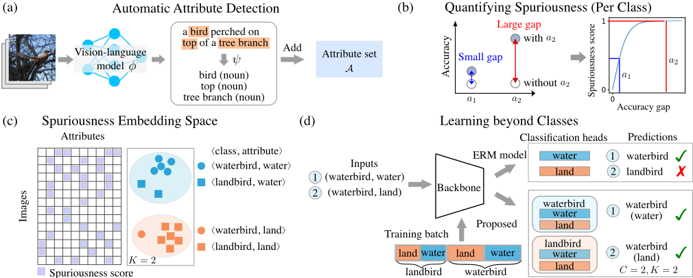
1. Generating text descriptions. We use a pre-trained VLM ϕ to generate text descriptions of images without human supervisions. Since the model is general-purposed and is not fine-tuned on target datasets, it can discover general objects and patterns. For example, in Figure 1(a), besides the class object bird, the model also detects tree branch.
2. Extracting informative words. We detect attributes by identifying nouns and adjectives from text descriptions as these types of words are informative in representing objects and patterns in images. We use an automatic procedure ψ (Section 5) to extract these informative words from the text descriptions obtained in the first step. For example, we extract bird, top, and tree branch from the description shown in Figure 1(a). We add the detected attributes to a set A as the set of all attributes detected from the images.
Remark: The VLM ϕ is only used for the one-time data preparation, i.e., detecting attributes from the training data; it does not involve in predictions. The inductive bias in ϕ only affects what attributes are detected. For example, it may inaccurately describe a lemon on a tree as a yellow bird (not self-explanatory). It is our algorithmic design introduced later that effectively mitigates a classifier's reliance on spurious correlations, even though some extracted words may not be self-explanatory in representing certain kinds of features.
Quantifying Spuriousness
A detected attribute in A may form a vague spurious correlation with a class, since it may not exist in images or some attributes are not spurious and represent class objects. More importantly, not all correlations are exploited by a classifier for predictions. To quantify the likelihood of a class-attribute correlation being spurious and used by a classifier, i.e., spuriousness of the correlation, we propose a novel metric, termed spuriousness score, that unifies the above cases.
Our spuriousness score for ⟨c, a⟩ is motivated by the observation that the classifier fθ will generalize poorly on samples of class c without the attribute a if fθ excessively relies on a for predicting the class c. Intuitively, the score will be higher if fθ has a larger performance discrepancy on images with and without a and vice versa. We formally define our spuriousness score for ⟨c, a⟩ as follows.
Definition 1 (Spuriousness score): Given a class c ∈ C, an attribute a ∈ A, and a classifier fθ trained on Dtr, the spuriousness of ⟨c, a⟩ is calculated as follows,
with γ(a, c; fθ, Dtr) = 0 when D⟨c,ˆa⟩ tr = ∅ or D⟨c,a⟩ tr = ∅, where D⟨c,a⟩ tr ⊂ Dtr denotes the subset of all training samples from class c with the attribute a, D⟨c,ˆa⟩ tr ⊂ Dtr denotes the subset of all training samples from class c without the attribute a, M(·; fθ) denotes the classification accuracy of fθ on a given set of samples, and Abs(·) denotes taking the absolute value. Using log(·) avoids encountering extreme values from the division, and tanh(Abs(·)) bounds the score in the range from 0 to 1. Figure 1(b) gives an example. Other designs of the score are explored in Appendix.
Remark: The score depends on both the training data and the classifier. Consider the two corner cases: when D⟨c,ˆa⟩ tr = ∅, a is always associated with c in Dtr, e.g., a is a class object; and when D⟨c,a⟩ tr = ∅, a and c are not associated, i.e., no samples correspond to the association between a and c. In both cases, the spuriousness score is zero as they do not fit in our description of spurious correlations. We exclude such attributes fromA. Moreover, the Abs(·) operator implies that when the fraction in Eq. (2) is lower than 1, i.e., a leads to incorrect predictions other than c and results in a small nominator, ⟨c, a⟩ still has a high spuriousness score as it also represents a robustness pitfall.
With the spuriousness score, we can quantify the impact of the correlation between the detected attribute a and the class c on the performance of the classifier fθ. The lower the spuriousness score, the less fθ relies on attribute a in its prediction, thus the more robust the classifier is.
4.2 Spuriousness-Guided Training Data Relabeling
Applying our spuriousness score (Eq. (2)) to all the possible correlations between the classes and the detected attributes, we can holistically characterize the spuriousness of images by showing how likely correlations relevant to an image are exploited by the classifier in predicting the image's label. To analyze the spuriousness of all the training images and pinpoint the robustness pitfalls of the classifier, we propose spuriousness embedding, which is defined as follows.
Definition 2 (Spuriousness embedding): Given an image x with label y, a classifier fθ, the detected attribute set A with NA attributes, a VLM ϕ, an attribute extraction procedure ψ, and the training set Dtr, we design the spuriousness embedding for (x, y), denoted as SE(x, y), as a NA-dimensional vector, whose ia-th element is defined as follows,
where a denotes an attribute of x, ia denotes the dimension index of SE(x, y) that corresponds to a, and 1{·} is the indicator function that equals one if the condition in the subscript is true and equals zero otherwise.
With spuriousness embeddings, we embed all images in Dtr in the spuriousness embedding space. Each point in the space represents both an image and a vector characterizing an individual spurious prediction behavior of fθ in using relevant class-attribute correlations to predict the image.
In the ideal scenario, a robust classifier produces all zero vectors in the space; practically, we expect to observe a dispersed distribution of points as the classifier does not excessively rely on specific spurious prediction behaviors. In contrast, a biased classifier tends to produce an uneven distribution of points from the same class. We demonstrate in Figure 1(c) with two clusters of similar prediction behaviors frequently used in predictions, i.e., using the water or land attributes. The partition based on the spuriousness of the images separates same-class samples unevenly, exposing potential prediction failure modes of the classifier, such as predicting a waterbird image with a land background as a landbird.
Therefore, we cluster images into K clusters in the spuriousness embedding space across different classes to capture potential failure modes in classification. Here, K is a hyperparameter and is controlled by our design choice. Formally, we represent the above process as follows,
where pK(x, y) is the cluster label for (x, y), and CLU denotes a clustering algorithm. In this paper, we use KMeans as CLU. Now, pK(x, y) summarizes similar prediction behaviors that may be used by the classifier for predictions. For example, the blue cluster in Figure 1(c) represents using the general attribute water for predicting waterbird, including using specific attributes such as pond and river.
We use the cluster labels pK(x, y) to guide the debiasing of the classifier by relabeling the training data with fine-grained labels formulated with pK(x, y) and y, which we unify as one symbol gK(x, y) = pK(x, y) + (y - 1) · K (y starts with 1).
4.3 Learning beyond Classes
To effectively use the relabeled training data for learning robust classifiers, we propose two novel strategies along with training and inference procedures in the following.
Diversifying Outputs of the Classifier
The constructed training labels instruct the classifier that multiple prediction behaviors for the same class should lead to a correct and consistent prediction outcome. To achieve this, we diversify the outputs of the classifier from predicting class labels to distinguishing between different prediction behaviors for the same class. In this way, the classifier is not only aware of other attributes leading to the same class, but also encouraged to discover more robust features for predictions.
Specifically, we separate fθ into a backbone eθ1 and a Cway classification head qθ2 , i.e, fθ = qθ2 ◦ eθ1 , where C is the number of classes, and the parameters θ = θ1 ∪ θ2. Then, we replace qθ2 with hθ3 which is a (K · C)-way classification head, resulting in a transformed model ˜ f˜ θ = hθ3 ◦ eθ1 with ˜ θ = θ3 ∪ θ1. Each output of ˜ f˜ θ corresponds to a combination of class c and cluster label k. Figure 1(d) gives an example with K = 2 and C = 2. In this example, instead of predicting two classes, i.e., waterbird and landbird, we replace the classification head of the ERM model with a new classification head to predict the correlations: ⟨waterbird, water⟩, ⟨waterbird, land⟩, ⟨landbird, water⟩, and ⟨landbird, land⟩.
Balancing Training Data
As discussed in Section 4.2, different prediction behaviors may correspond to uneven numbers of samples, which may bias the predictions of the adapted classifier. To address this, we consider within-class and cross-class balancing strategies. Within-class balancing. We sample K equal-sized training sets Bk c ⊆ G k c with images from class c and K different clusters, where G k c is defined as
In this way, we assign equal importance to predicting the K clusters within the class c. We ignore G k c when it is empty.
Cross-class balancing. Considering that predictions for different classes may show varied reliance on spurious correlations, we additionally balance the size of Bc = ∪Kk=1Bk c . Specifically, for each class c, we calculate the variance of cluster sizes within class c, i.e., σ2 c = V ar({|G k c | |k = 1, . . . ,K}), where | · | denotes the size of a set, and V ar(·) denotes the variance of a set of numbers. The variance measures the degree of imbalanced prediction behaviors for class c. We control the size of Bc based on σc such that we sample more training data for a class that exhibits a larger degree of imbalanced prediction behaviors. Concretely, given the batch size B, we set |Bc| = B · ρc, |Bk c | = B · ρc/K, where ρc = log(σc + 1)/ ∑Cc′=1 log(σc′ + 1), and we use log(σc + 1) to avoid encountering extreme values.
Training and Inference
The overall learning objective is as follows,
It is possible that after training on Eq. (6), the model develops reliance on other spurious correlations. Therefore, we iteratively update the spuriousness scores based on the updated model and perform the above mitigation procedure again. We call this method Learning beyond Classes (LBC). The whole procedure is listed in Algorithm 1 in Appendix.
Model selection. Given a validation set Dval without group labels, we develop a selection metric called pseudo unbiased validation accuracy Accpseudo unbiased to select the best model during training. Specifically, we group the validation data based on the existence of the detected attribute a, i.e.,
Then, we calculate Accpseudo unbiased as the average over the accuracy on Da val as follows,
During inference, the predicted label is calculated as ˆ c = ⌈(argmaxc ˜ f˜ θ (x))/K⌉, where ⌈c⌉ denotes taking the smallest integer greater than or equal to c.
5 Experiment
5.1 Datasets
Waterbirds [Sagawa et al., 2019] is a dataset for recognizing waterbirds and landbirds. It is generated synthetically by combining images of the two kinds of birds from the CUB dataset [Welinder et al., 2010] and the backgrounds, water and land, from the Places dataset [Zhou et al., 2017].
CelebA [Liu et al., 2015] is a large-scale image dataset of celebrity faces. The task is to identify hair color, non-blond or blond, with male and female as the spurious attributes.
ImageNet-9 [Xiao et al., 2021] comprises images with different background and foreground signals, which can be used to assess how much models rely on image backgrounds. This dataset is a subset of ImageNet [Deng et al., 2009] containing nine super-classes.
ImageNet-A [Hendrycks et al., 2021] is a dataset of realworld images, adversarially curated to test the limits of classifiers such as ResNet-50. While these images are from standard ImageNet classes [Deng et al., 2009], their complexity increases the challenge, often causing misclassifications in multiple models. We use this dataset to test the robustness of a classifier after training it on ImageNet-9.
NICO [He et al., 2021] is designed for non-independent and identically distributed and out-of-distribution image classification, simulating real-world scenarios where testing distributions differ from training ones. It labels images with both main concepts and contexts (e.g., 'dog on grass'), enabling studies on transfer learning, domain adaptation, and generalization.
Details of the dataset settings are shown in Appendix.
5.2 Experimental Setup
Spurious attribute detection. We generate text descriptions for images using a pre-trained vision-language model [NLP Connect, 2022], which has an encoder-decoder structure where the encoder is a vision transformer [Dosovitskiy et al., 2020] and the decoder is the GPT-2 [Radford et al., 2019] language model. We set the maximum length of the sequence to be generated as 16 and the number of beams for beam search to 4. After generating text descriptions for test images, we use Spacy (https://spacy.io/) to extract nouns and adjectives from the descriptions automatically. We additionally filter out words with frequencies less than 10 to remove potential annotation noise. In our experiments, we only need to do this procedure once for each dataset.
Training settings. We use ResNet-50 and ResNet-18 as the backbone networks. For each dataset, we first train an ERM model, which is first initialized with ImageNet pre-trained weights, for 100 epochs. We set the learning rate to 0.001 which decays following a cosine annealing scheduler and use an SDG optimizer with 0.9 momentum and 10-4 weight decay. Then, we use the ERM-trained models as the initial models for our LBC training. Standard data augmentations are used in LBC to effectively mitigate spurious correlations that are not typically captured by VLMs, such as sizes and orientations. For all the datasets, we fix the learning rate to 0.0001 and the batch size to 128. We sample 20 batches per epoch and train for 50 epochs. The cluster size K is set to 3. We report our results averaged over 5 runs. We provide training details in the Appendix. All experiments are conducted on NVIDIA RTX 8000 GPUs 1 .
Evaluation metrics. We adopt different evaluation metrics on different datasets. For a dataset with group labels defined by classes and biased attributes, we partition the test data into groups. Average accuracy measures the overall performance of a classifier on the test data; however, it may be dominated by the majority group of samples with certain biases that the classifier may heavily rely on for predictions. Therefore, we mainly focus on the worst-group accuracy which is a widely accepted robustness measure that gives the lower-bound performance of a classifier on various dataset biases. To measure the tradeoff between the average and worst accuracy, we additionally calculate the gap between the two metrics. For datasets without group labels, we report different kinds of average accuracies on specifically designed test sets, which we will explain in the respective sections.
1 Our code is available at https://github.com/gtzheng/LBC.
| Method | Backbone | Group information | CelebA | Waterbirds | |||||
|---|---|---|---|---|---|---|---|---|---|
| Train | Validation | Worst(↑) | Average(↑) | Gap(↓) | Worst(↑) | Average(↑) | Gap(↓) | ||
| GroupDRO [Sagawa et al., 2019] | ResNet-50 | ✓ | ✓ | 88.9 | 92.9 | 4.0 | 91.4 | 93.5 | 2.1 |
| LfF [Nam et al., 2020] | ResNet-50 | ✗ | ✓ | 78.0 | 85.1 | 7.1 | 78.0 | 91.2 | 13.2 |
| CVaR DRO [Levy et al., 2020] | ResNet-50 | ✗ | ✓ | 64.4 | 82.5 | 18.1 | 75.9 | 96.0 | 20.1 |
| JTT [Liu et al., 2021] | ResNet-50 | ✗ | ✓ | 81.1 | 88.0 | 6.9 | 86.7 | 93.3 | 6.6 |
| DFR [Kirichenko et al., 2023] | ResNet-50 | ✗ | ✓ | 69.4±1.4 | 93.3±0.1 | 23.9±1.3 | 80.2±2.3 | 92.1±0.6 | 11.9±2.7 |
| LBC (Ours) | ResNet-50 | ✗ | ✓ | 87.4±1.8 | 92.4±0.3 | 5.0±2.1 | 88.1±1.4 | 94.1±0.3 | 6.0±1.7 |
| ERM | ResNet-50 | ✗ | ✗ | 45.7 | 95.5 | 49.8 | 66.4 | 90.2 | 23.8 |
| LfF [Nam et al., 2020] | ResNet-50 | ✗ | ✗ | 24.4 | 85.1 | 60.7 | 44.1 | 91.2 | 47.1 |
| CVaR DRO [Levy et al., 2020] | ResNet-50 | ✗ | ✗ | 36.1 | 82.5 | 46.4 | 62.0 | 95.2 | 33.2 |
| JTT [Liu et al., 2021] | ResNet-50 | ✗ | ✗ | 40.6 | 88.0 | 47.4 | 62.5 | 93.3 | 30.8 |
| DivDis [Lee et al., 2022] | ResNet-50 | ✗ | ✗ | 55.0 | 90.8 | 35.8 | 81.0 | 90.7 | 9.7 |
| MaskTune [Asgari et al., 2022] | ResNet-50 | ✗ | ✗ | 78.0±1.2 | 91.3±0.1 | 13.3±1.3 | 86.4±1.9 | 93.0±0.7 | 6.6±2.6 |
| DFR [Kirichenko et al., 2023] | ResNet-50 | ✗ | ✗ | 46.0 | 95.8 | 49.8 | 77.4 | 92.1 | 14.7 |
| LBC (Ours) | ResNet-50 | ✗ | ✗ | 81.2±1.5 | 92.2±0.3 | 11.0±1.8 | 87.3±1.8 | 93.2±0.9 | 5.9±2.7 |
| Class | Attributes |
|---|---|
| landbird | pool , boat , building , pond , surfboard , sandy , beach , water , body, frisbee |
| waterbird | stream , forest , building , pile, front, middle, animal, photo, tree , branch |
5.3 Effectiveness of Spuriousness Score
We calculated the spuriousness scores for the correlations between all the detected attributes and classes in the Waterbirds dataset and selected the top-10 attributes with the highest spuriousness scores for each class. Table 2 shows that these attributes are mostly relevant to water and land backgrounds, which are spurious by design. Interestingly, our spuriousness score can find attributes in one class that are heavily exploited to predict some other class. For example, pool from landbird is detected in images of landbird with a pool, but it tends to bias the predictions toward waterbird since it is relevant to water backgrounds. As discussed in Section 4.1, this arises from the Abs operator in our definition of spuriousness score in Eq. (2): when the nominator term is much smaller than the denominator term, e.g., when a=pool and c=landbird, the spuriousness score is still high. Examples from other datasets are shown in the Appendix.
5.4 LBCReduces Reliance on Spurious Correlations
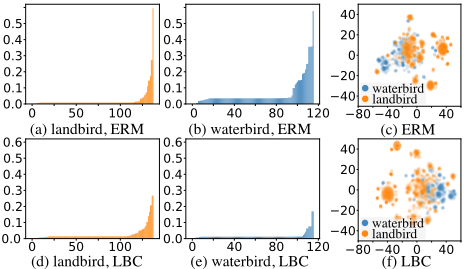
To show the efficacy of our LBC method in learning a model robust to spurious correlations, we quantitatively and qualitatively demonstrate this by using spuriousness scores and visualizations of spuriousness embeddings, respectively. We first calculated the spuriousness scores for the class-attribute correlations based on an ERM and our LBC-trained models. Comparing the results between Figure 2(a) and Figure 2(d), as well as between Figure 2(b) and Figure 2(e), we observe that LBC significantly reduces the spuriousness scores of the correlations between the detected attributes and the two classes. Moreover, the spuriousness embeddings, which represent images with different prediction behaviors, become more dispersed in Figure 2(f) than in Figure 2(c). This indicates that LBC successfully mitigates the ERM classifier's reliance on certain prediction behaviors and diversifies the prediction behaviors for different classes.
5.5 Comparison with ExistingMethods
Datasets with group labels. Table 1 gives the results on the CelebA and Waterbirds datasets in two settings. In the first setting where only the group labels of the validation data are used, our method achieves the best worst-group accuracies and the best gaps between the average and the worst-group accuracies on the two datasets, striking a favorable balance between the robustness of the classifier and its overall performance. Our worst-group accuracies are also close to the upper bounds established by GroupDRO, while our average accuracies are competitive or better than those of GroupDRO. In our main setting where no group labels are available, our method outperforms the baselines with the best worst-group accuracies and worst-average gaps. More significantly, our method is most robust in terms of the least drops in worstgroup accuracy when switching from the first setting to the second one. This shows the effectiveness of our designed model selection metric in selecting robust models.
| Method | ImageNet-9 | ImageNet-A | |
|---|---|---|---|
| SA Validation(↑) | Unbiased(↑) | Test(↑) | |
| StylisedIN [Geirhos et al., 2018] LearnedMixin [Clark et al., 2019] RUBi [Cadene et al., 2019] | ✓ 88.4±0.5 ✓ 64.1±4.0 ✓ 90.5±0.3 | 86.6±0.6 62.7±3.1 88.6±0.4 | 24.6±1.4 15.0±1.6 27.7±2.1 |
| ERM ReBias [Bahng et al., 2020] LfF [Nam et al., 2020] | ✗ 90.8±0.6 | 88.8±0.6 | 24.9±1.1 |
| ✗ 91.9±1.7 | 90.5±1.7 | 29.6±1.6 | |
| ✗ 86.0 | 85.0 | 24.6 | |
| CaaM [Wang et al., 2021] | ✗ 95.7 | 95.2 | 32.8 |
| SSL+ERM [Kim et al., 2022] | ✗ | 93.18±0.04 | 34.21±0.49 |
| 2022] | 94.18±0.07 94.03±0.23 | 35.97±0.49 | |
| LWBC [Kim et al., LBC (Ours) | ✗ ✗ 96.97±0.17 | 93.04±0.32 96.03±0.12 | 40.63±1.79 |
Datasets with texture biases. Experiments on ImageNet-9 and ImageNet-A test how much a classifier relies on the spurious texture bias. In Table 3, texture group labels [Bahng et al., 2020; Kim et al., 2022] are used as the spurious attribute labels. The "Validation" denotes the average accuracy on the validation set, "Unbiased" denotes the average accuracy over several texture groups, and "Test" denotes the average accuracy on the ImageNet-A dataset which contains misclassified samples by an ImageNet-trained model. Our method outperforms other methods on the three metrics, showing that our method is effective in mitigating a classifier's reliance on texture biases and correcting its failure modes in classification.
Dataset with object-context correlations. The NICO dataset is created to evaluate a classifier's reliance on objectcontext correlations. Images in the training set are long-tailed distributed in the sense that an object class has exponentially decreasing numbers of images that correlate with the contexts. In Table 4, "Validation" denotes the average accuracy on the validation set, and "Test" denotes the average accuracy on the test set. Both validation and test sets contain not only existing object-context correlations but also unseen ones. Our method effectively mitigates the reliance on object-context correlations and achieves the best on the two metrics.
5.6 Ablation Study
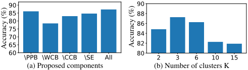
We first analyzed the effectiveness of the four proposed components: (1) predicting prediction behaviors (PPB), (2) within-class balancing (WCB), (3) cross-class balancing, and (4) spuriousness embeddings (SE). We modify one component and observe the worst-group accuracies achieved by the remaining ones. In Figure 3(a), \PPB denotes that we keep the original classifier to predict classes, \WCB denotes that we randomly sample from the same class, \CCB denotes that we equally sample images with different identified prediction behaviors, and \SE denotes that we use binary attribute embeddings (i.e., SE(x, y)[ia] = 1a∈ψ(ϕ(x)) in Eq. (3)) for images. We observe that all four components positively contribute to our method since replacing any one of them results in reduced accuracy. Among the four components, balanced data sampling (WCB and CCB), especially WCB, is most critical to our method. Figure 3(b) shows that a large K exceeding 10 has suboptimal worst-group accuracies and that when K = 2, it limits the discovery of diverse prediction behaviors. Typically, K = 3 works for most of the cases. We also showed in Appendix that the detected attributes from the VLM alone do not contain information effective for improving a classifier's robustness to spurious correlations.
| NICO | |||
|---|---|---|---|
| Method | SA | Validation(↑) | Test(↑) |
| RUBi [Cadene et al., 2019] | ✓ | 43.86 | 44.37 |
| IRM [Arjovsky et al., 2019] | ✓ | 40.62 | 41.46 |
| ERM | ✗ | 43.77 | 42.61 |
| CBAM [Woo et al., 2018] | ✗ | 42.15 | 42.46 |
| ReBias [Bahng et al., 2020] | ✗ | 44.92 | 45.23 |
| LfF [Nam et al., 2020] | ✗ | 41.83 | 40.18 |
| CaaM [Wang et al., 2021] | ✗ | 46.38 | 46.62 |
| SSL+ERM [Kim et al., 2022] | ✗ | 55.63±0.54 | 52.24±0.27 |
| LWBC [Kim et al., 2022] | ✗ | 56.05±0.45 | 52.84±0.31 |
| LBC (Ours) | ✗ | 68.26±2.15 | 65.34±2.54 |
6 Conclusion
We completely removed the barrier of requiring expert knowledge and human annotations for spurious correlation mitigation by proposing a self-guided framework. Our framework incorporates an automatic approach empowered by a VLM to detect attributes in images and quantifies their spuriousness with class labels. We formulated a spuriousness embedding space based on the spuriousness scores to identify distinct prediction behaviors of a classifier. We trained the classifier to recognize the identified prediction behaviors with balanced training data. Experiments showed that our framework improves the robustness of a classifier against spurious correlations without knowing them in the data.
Acknowledgments
This work is supported in part by the US National Science Foundation under grants 2217071, 2213700, 2106913, 2008208, 1955151.
@inproceedings{ijcai2024p619,
  title     = {Learning Robust Classifiers with Self-Guided Spurious Correlation Mitigation},
  author    = {Zheng, Guangtao and Ye, Wenqian and Zhang, Aidong},
  booktitle = {Proceedings of the Thirty-Third International Joint Conference on
               Artificial Intelligence, {IJCAI-24}},
  publisher = {International Joint Conferences on Artificial Intelligence Organization},
  editor    = {Kate Larson},
  pages     = {5599--5607},
  year      = {2024},
  month     = {8},
  note      = {Main Track},
  doi       = {10.24963/ijcai.2024/619},
  url       = {https://doi.org/10.24963/ijcai.2024/619},
}
TY - CPAPER TI - Learning Robust Classifiers with Self-Guided Spurious Correlation Mitigation AU - Zheng, Guangtao AU - Ye, Wenqian AU - Zhang, Aidong T2 - Proceedings of the Thirty-Third International Joint Conference on Artificial Intelligence, IJCAI-24 PB - International Joint Conferences on Artificial Intelligence Organization PY - 2024 SP - 5599 EP - 5607 DO - 10.24963/ijcai.2024/619 UR - https://doi.org/10.24963/ijcai.2024/619 ER -Copied
Machine-readable versions of this paper, for tools and AI agents:





