
SACNN: Self Attention-based Convolutional Neural Network for Fraudulent Behaviour Detection in Sports
Proceedings of the Thirty-Third International Joint Conference on Artificial Intelligence. Main Track. Pages 6017-6025.
https://doi.org/10.24963/ijcai.2024/665
Keywords
- Multidisciplinary Topics and Applications: MTA: Sports
- Machine Learning: ML: Applications
- AI Ethics, Trust, Fairness: ETF: Societal impact of AI
Abstract
Doping practices in sports by unscrupulous athletes have been an important societal issue for several decades. Recently, sample swapping has been raised as a potential practice performed by athletes to swap their doped samples with clean samples to evade the positive doping test. So far, the only proven method to detect such cases is by performing DNA analysis on samples. However, it is expensive and time-consuming, which goes beyond the budgetary limits of anti-doping organisations when implementing to all the samples collected during sports events. Therefore, in this paper, we propose a self attention-based convolutional neural network (SACNN) that incorporates both spatial and temporal behaviour of the longitudinal profile and generates embedding maps for solving the fraud detection problem in sports. We conduct extensive experiments on the real-world datasets. The result shows that SACNN outperforms other state-of-the-art baseline models for sequential anomaly detection. Moreover, we conduct a study with domain experts on real-world profiles using both DNA analysis and our proposed method; the result demonstrates the effectiveness of our proposed method and the impact it could bring to the society.
- [Callaway, 2011] Ewen Callaway. Sports doping: Racing just to keep up. Nature, 475(7356):283-285, 2011.
- [Chen et al., 2021] Chun-Fu Richard Chen, Rameswar Panda, Kandan Ramakrishnan, Rogerio Feris, John Cohn, Aude Oliva, and Quanfu Fan. Deep analysis of cnn-based spatio-temporal representations for action recognition. In 2021 IEEE/CVF Conference on Computer Vision and Pattern Recognition (CVPR), pages 6161-6171, 2021.
- [Cheng et al., 2020] Dawei Cheng, Sheng Xiang, Chencheng Shang, Yiyi Zhang, Fangzhou Yang, and Liqing Zhang. Spatio-temporal attention-based neural network for credit card fraud detection. Proceedings of the AAAI Conference on Artificial Intelligence, 34(01), Apr. 2020.
- [Elbayad et al., 2018] Maha Elbayad, Laurent Besacier, and Jakob Verbeek. Pervasive attention: 2D convolutional neu- ral networks for sequence-to-sequence prediction. In Pro- ceedings of the 22nd Conference on Computational Natu- ral Language Learning, pages 97-107, Brussels, Belgium, October 2018.
- [Ellore et al., 2020] Anish Ellore, Sanket Mishra, and Chit- taranjan Hota. Sequential Anomaly Detection Using Feed- back and Prioritized Experience Replay, pages 245-260. 12 2020.
- [Gu et al., 2021] Ran Gu, Guotai Wang, Tao Song, Rui Huang, Michael Aertsen, Jan Deprest, Sebastien Ourselin, Tom Vercauteren, and Shaoting Zhang. CA-net: Com- prehensive attention convolutional neural networks for ex- plainable medical image segmentation. IEEE Transactions on Medical Imaging, 40(2):699-711, feb 2021.
- [Higgins et al., 2017] Irina Higgins, Loic Matthey, Arka Pal, Christopher Burgess, Xavier Glorot, Matthew Botvinick, Shakir Mohamed, and Alexander Lerchner. beta-VAE: Learning basic visual concepts with a constrained varia- tional framework. In International Conference on Learn- ing Representations, 2017.
- [Kobierecka and Kobierecki, 2019] Anna Kobierecka and Michał Kobierecki. The negative implications of russia's doping scandal on the country's international image. East- ern Review, 8:161-182, 12 2019.
- [Li et al., 2021] Pengfei Li, Peixiang Zhong, Kezhi Mao, Dongzhe Wang, Xuefeng Yang, Yunfeng Liu, Jianxiong Yin, and Simon See. Act: an attentive convolutional trans- former for efficient text classification. Proceedings of the AAAI Conference on Artificial Intelligence, 35(15), May 2021.
- [Lin et al., 2020] Shuyu Lin, Ronald Clark, Robert Birke, Sandro Schönborn, Niki Trigoni, and Stephen Roberts. Anomaly detection for time series using vae-lstm hy- brid model. In ICASSP 2020 -2020 IEEE International Conference on Acoustics, Speech and Signal Processing (ICASSP), pages 4322-4326, 2020.
- [Liu et al., 2008] Fei Tony Liu, Kai Ming Ting, and Zhi-Hua Zhou. Isolation-based anomaly detection. In 2008 Eighth IEEE International Conference on Data Mining, pages 413-422. IEEE, 2008.
- [McLaren, 2016] Richard H. McLaren. Wada investigation of sochi allegations: The independent person 2nd report. World Anti-Doping Agency, Dec 2016.
- [Nikolentzos et al., 2020] Giannis Nikolentzos, Antoine Tixier, and Michalis Vazirgiannis. Message passing attention networks for document understanding. Proceed- ings of the AAAI Conference on Artificial Intelligence, 34(05):8544-8551, Apr. 2020.
- [Piper et al., 2021] Thomas Piper, Hans Geyer, Nadine Haenelt, Frank Hülsemann, Wilhelm Schaenzer, and Mario Thevis. Current insights into the steroidal module of the athlete biological passport. International Journal of Sports Medicine, 42, 05 2021.
- [Rahman et al., 2022a] Maxx Richard Rahman, Jacob Be- jder, Thomas Christian Bonne, Andreas Breenfeldt Ander- sen, Jesús Rodríguez Huertas, Reid Aikin, Nikolai Baas- trup Nordsborg, and Wolfgang Maass. Detection of ery- thropoietin in blood to uncover doping in sports using ma- chine learning. In 2022 IEEE International Conference on Digital Health (ICDH), pages 193-201, 2022.
- [Rahman et al., 2022b] Maxx Richard Rahman, Thomas Piper, Hans Geyer, Tristan Equey, Norbert Baume, Reid Aikin, and Wolfgang Maass. Data analytics for uncovering fraudulent behaviour in elite sports. In 2022 International Conference on Information System (ICIS), 2022.
- [Rahman et al., 2023] Maxx Richard Rahman, Mohammed Hussain, Thomas Piper, Hans Geyer, Tristan Equey, Nor- bert Baume, Reid Aikin, and Wolfgang Maass. Modelling metabolism pathways using graph representation learning for fraud detection in sports. In 2023 IEEE International Conference on Digital Health (ICDH), pages 158-168, 2023.
- [Rudenko, 2014] Rudenko. Main modern problems of dop- ing in sport. Pedagogics, Psychology, Medical-Biological Problems of Physical Training and Sports, 6, 04 2014.
- [Schiffer et al., 2019] Lina Schiffer, Lise Barnard, Eliza- beth S Baranowski, Lorna C Gilligan, Angela E Taylor, Wiebke Arlt, Cedric HL Shackleton, and Karl-Heinz Stor- beck. Human steroid biosynthesis, metabolism and excre- tion are differentially reflected by serum and urine steroid metabolomes: A comprehensive review. The Journal of steroid biochemistry and molecular biology, 194:105439, 2019.
- [Schlegl et al., 2017] Thomas Schlegl, Philipp Seeböck, Se- bastian M. Waldstein, Ursula Schmidt-Erfurth, and Georg Langs. Unsupervised anomaly detection with generative adversarial networks to guide marker discovery. In Infor- mation Processing in Medical Imaging, pages 146-157, Cham, 2017. Springer International Publishing.
- [Shen et al., 2018] Tao Shen, Tianyi Zhou, Guodong Long, Jing Jiang, Shirui Pan, and Chengqi Zhang. Disan: Di- rectional self-attention network for rnn/cnn-free language understanding. Proceedings of the AAAI Conference on Artificial Intelligence, 32(1), Apr. 2018.
- [Sípoli Marques et al., 2005] Marlice Aparecida Sípoli Mar- ques, Lucia Meneses Pinto Damasceno, Henrique Marcelo Gualberto Pereira, Concy Maya Caldeira, Bianca Faria Pereira Dias, Daniela de Giacomo Vargens, Nívea Dias Amoedo, Rosana Oliveira Volkweis, Rosane Oliveira Volkweis Viana, Franklin David Rumjanek, and Fran- cisco Radler Aquino Neto. Dna typing: an accessory ev- idence in doping control. J Forensic Sci, 50(3):587-592, May 2005.
- [Song et al., 2019] Weiping Song, Chence Shi, Zhiping Xiao, Zhijian Duan, Yewen Xu, Ming Zhang, and Jian Tang. AutoInt. In Proceedings of the 28th ACM Inter- national Conference on Information and Knowledge Man- agement. ACM, nov 2019.
- [Sottas et al., 2006] Pierre-Edouard Sottas, Norbert Baume, Christophe Saudan, Carine Schweizer, Matthias Kamber, and Martial Saugy. Bayesian detection of abnormal values in longitudinal biomarkers with an application to T/E ratio. Biostatistics, 8(2):285-296, 06 2006.
- [Thevis et al., 2012] Mario Thevis, Hans Geyer, Gerd Sig- mund, and Wilhelm Schänzer. Sports drug testing: An- alytical aspects of selected cases of suspected, purported, and proven urine manipulation. Journal of Pharmaceuti- cal and Biomedical Analysis, 57:26-32, 2012.
- [Tran et al., 2015] Du Tran, Lubomir Bourdev, Rob Fer- gus, Lorenzo Torresani, and Manohar Paluri. Learning spatiotemporal features with 3d convolutional networks. pages 4489-4497, 12 2015.
- [Van Renterghem et al., 2013] Pieter Van Renterghem, Pierre-Edouard Sottas, Martial Saugy, and Peter Van Eenoo. Statistical discrimination of steroid profiles in doping control with support vector machines. Analytica Chimica Acta, 768:41-48, 2013.
- [Vaswani et al., 2017] Ashish Vaswani, Noam Shazeer, Niki Parmar, Jakob Uszkoreit, Llion Jones, Aidan N Gomez, Ł ukasz Kaiser, and Illia Polosukhin. Attention is all you need. In Advances in Neural Information Processing Sys- tems, volume 30.
- Curran Associates, Inc., 2017.
- [WADA, 2005] WADA. Anti-doping administration management system (adams). https://www.wada- ama.org/en/what-we-do/adams, 2005. Accessed: 2023- 11-07. Link
- [WADA, 2021] WADA. Measurement and reporting of en- dogenous anabolic androgenic steroid (eaas) markers of the urinary steroid profile. In WADA Technical Document -TD2021EAAS, 2021.
- [Wang et al., 2022] Wei-Yao Wang, Teng-Fong Chan, Wen- Chih Peng, Hui-Kuo Yang, Chih-Chuan Wang, and Yao- Chung Fan. How is the stroke? inferring shot influence in badminton matches via long short-term dependencies. ACM Transactions on Intelligent Systems and Technology, 14(1):1-22, 2022.
- [Wilkes et al., 2018] Edmund H Wilkes, Gill Rumsby, and Gary M Woodward. Using Machine Learning to Aid the Interpretation of Urine Steroid Profiles. Clinical Chem- istry, 64(11):1586-1595, 11 2018.
- [Xu and Cai, 2019] Jingyun Xu and Yi Cai. Incorporating context-relevant knowledge into convolutional neural net- works for short text classification. Proceedings of the AAAI Conference on Artificial Intelligence, 33(01):10067- 10068, Jul. 2019.
- [Zhang et al., 2020] Yanghao Zhang, Wenjie Ruan, Fu Wang, and Xiaowei Huang. Generalizing univer- sal adversarial attacks beyond additive perturbations. In 2020 IEEE International Conference on Data Mining (ICDM), pages 1412-1417, 2020.
- [Zhao and Hryniewicki, 2018] Yue Zhao and Maciej K. Hryniewicki. Xgbod: Improving supervised outlier de- tection with unsupervised representation learning. In 2018 International Joint Conference on Neural Networks (IJCNN), pages 1-8, 2018.
- [Zhao et al., 2019] Yue Zhao, Zain Nasrullah, Maciej K Hryniewicki, and Zheng Li. LSCP: locally selective com- bination in parallel outlier ensembles. In Proceedings of the 2019 SIAM International Conference on Data Mining, SDM 2019, pages 585-593, May 2019.
- [Zhao et al., 2021] Yue Zhao, Xiyang Hu, Cheng Cheng, Changlin Wan, Wen Wang, Jianing Yang, Haoping Bai, Zheng Li, Cao Xiao, Yunlong Wang, Zhi Qiao, J. Sun, and Leman Akoglu. Suod: Accelerating large-scale unsuper- vised heterogeneous outlier detection. 01 2021.
References were extracted automatically from the PDF and may contain errors.
Full text extracted automatically from the PDF; figures, tables and equations may differ. The PDF is the version of record.
1 Introduction
Sports events, such as the Olympic Games or FIFA World Cup, attract the attention of billions of people around the world. However, the fraudulent behaviour by athletes to enhance their performance in these events raises many social issues due to ethical and moral reasons [Rudenko, 2014]. The impact of this can be seen at both individual and societal levels, e.g., disqualification of athletes, or even ban of a nation from competing in future events, etc. [Kobierecka and Kobierecki, 2019] Therefore, it is a global concern that follows international sporting events worldwide, and antidoping analysis is a crucial measure to fight against these activities in sports [Callaway, 2011]. During the recent investigation at the Olympic Games 2014 in Sochi, a new form of fraudulent activity was found. Some athletes try to swap/exchange their doped samples with another individual's clean sample to evade positive tests, this refers to 'sample swapping' [McLaren, 2016]. This simple but new form of fraudulent activity became a threat to the whole anti-doping decision-making organisation. The anti-doping organisation maintains a longitudinal profile of every athlete, which contains records of all the samples collected from that athlete so far for the doping tests.
The primary way to detect sample swapping is to perform DNA analysis across all the samples [S´ıpoli Marques et al., 2005]. However, it is expensive and time-consuming to be implemented on the longitudinal profile of all the athletes who participated in the sports events (economic costs of more than $300 million/year). Other methods include monitoring each sample and comparing them with reference ranges of the athlete to be able to detect unnaturally high values [Rahman et al., 2022b; Piper et al., 2021; Sottas et al., 2006]. However, this interpretation does not take into account two important aspects. 1) Temporal behaviour: the human body or metabolism evolves over time, and so does the athlete's performance. Therefore, defining a reference range based on the previously collected samples would add bias when comparing the new samples. 2) Spatial behaviour: each collected sample is used to determine different parameters representing different elements of human steroid metabolism pathway, which have both intrinsic and extrinsic dependency [Schiffer et al., 2019; Rahman et al., 2023]. Therefore, it is important to exploit this information when comparing the similarity of the samples within the longitudinal profile.
This scenario can be well represented as a multivariate sequential anomaly detection problem [Ellore et al., 2020], where we are interested in determining the anomalous sequence based on spatio-temporal patterns. Many existing models that deals with sequential anomaly were studied [Lin et al., 2020; Zhao et al., 2021; Schlegl et al., 2017]. However, all these models mainly focus on manually defining the feature space, and fails to automatically learn the joint impact of spatial and temporal behaviour. Recently developed attention mechanisms have shown the benefit of automatic feature learning [Vaswani et al., 2017; Song et al., 2019]. The performance of a convolution network on spatio-temporal feature learning is also demonstrated in a wide range of tasks [Chen et al., 2021; Tran et al., 2015]. Therefore, in this paper, we present an approach that jointly considers spatio-temporal behaviour by constructing embedding maps and captures intrinsic relationships from these maps to uncover hidden fraud patterns. During experiments with real-world datasets, we show that the results of the proposed model significantly outperform other state-of-the-art (SoTA) baseline models. Our model serves as an adaptive approach for the preliminary screening. In case of positive results, confirmatory DNA testing is performed to eliminate false positives, ensuring that no athlete faces unjust penalties without irrefutable evidence.
The main contributions of our work can be summarised as follows:
- We propose a novel architecture based on self-attention mechanism, convolution layers and adversarial attack for detecting fraudulent behaviour in sports by capturing the embeddings from the longitudinal profiles of athletes. To the best of our knowledge, this is the first time that a fraud detection problem in sports has been addressed by considering spatio-temporal behaviour.
- Our method is extensively evaluated on different realworld datasets collected by anti-doping organisation and associated laboratory. The experimental results show the efficacy of our proposed model, which could detect more fraud athletes with relatively high specificity compared with SoTA baseline models.
- We perform a case study to show the performance of the proposed model on the real world fraudulent athlete's profiles which were tested by DNA analysis.
2 RelatedWork
2.1 Attentional Convolution Neural Network
Many recent studies have shown the advantage of combining an attention mechanism with convolutional networks for a wide range of applications [Vaswani et al., 2017; Song et al., 2019], such as medical image segmentation [Gu et al., 2021], language understanding [Shen et al., 2018], etc. For instance, the attentional convolution network is well exploited in many NLP-related tasks, e.g. text classification [Li et al., 2021; Xu and Cai, 2019], sequence-to-sequence prediction [Elbayad et al., 2018], document understanding [Nikolentzos et al., 2020], etc. [Cheng et al., 2020] employed an attention model for learning spatio-temporal features in fraud detection. Our approach develops from a similar intuition and integrates an attention network to generate embedding maps that consider both spatial and temporal aspects and let convolutional filters learn the relationships from these embedding maps.
2.2 Detection of Fraudulent Behaviour in Sports
Detection of fraudulent activities like doping using machine learning is not new in the sports anti-doping community.
[Sottas et al., 2006] proposed a Bayesian approach for the detection of abnormal values in the longitudinal profiles. Several studies [Van Renterghem et al., 2013; Wilkes et al., 2018; Wang et al., 2022; Rahman et al., 2022a] used different ML algorithms for detecting anomalous samples in the profile. However, the problem of investigating sample swapping is not so far addressed by machine learning. Currently, it is mainly detected by laboratory-based methods. Studies like [Thevis et al., 2012; Piper et al., 2021] showed how different biochemical techniques like gas chromatography-mass spectrometry, DNA-STR analysis, etc., can be used to detect sample swapping. However, these methods ignore the joint feature learning on spatial and temporal relationships. The approach we present in this paper is radically different and addresses this problem.
3 Preliminaries
3.1 Sample
A sample x = {f1, f2, ..., fk} means a urine sample collected from the athlete for performing the doping test, where each element represents the metabolites in human steroid metabolism. This metabolism pathway is a biological mechanism that follows spatial relationship [Rahman et al., 2023]. Testing sample xT refers to the sample under consideration for the similarity check with other samples in the longitudinal profile.
3.2 Longitudinal Profile
A longitudinal profile of an athlete X = {x1, x2, ..., xn} refers to a sequence of samples collected from that athlete at different times, where n = total number of samples. When n = 2, we define it as limited longitudinal profile Xlim = {x1, x2}. In this case, it is difficult to compute x1 ∼ x2.
3.3 Fraudulent Behaviour
A fraudulent behaviour in this paper refers to when an athlete performs sample swapping, i.e. exchange their doped sample with a clean sample from another individual. In this case, if the collected sample is xT , then it will not match with other samples in the longitudinal profile.
For example, let us assume we have the longitudinal profiles of athletes X1 and X2, where athlete X1 has a clean profile, i.e., all the samples are similar to each other and athlete X2 has anamolous profile. Let us suppose the samples x4, and x7 of athlete X2 are under consideration, i.e. xT = {x4, x7} whether they are from the athlete X2 or swapped by the athlete to evade the positive doping test. It could also be possible that both the samples are from the same athlete other than X2 (i.e. x4, x7 ∈ X1) or even from different athletes (i.e. x4 ∈ X1, x7 ∈ X3). Therefore, the goal is to find whether the given sequence is anomalous or not in the collection of sequences. For that, we need an iterative algorithm that investigates the similarity of each sample with every testing sample in the longitudinal profile, using xT ∼ xi, ∀ xT , xi ∈ X. However, the prevalence of sample swapping in the real-world situation is very less compared to the clean athletic population. Therefore, this problem can be well formulated as anomaly detection problem in multivariate sequential data.
4 Self Attention-based Convolutional Neural Network (SACNN)
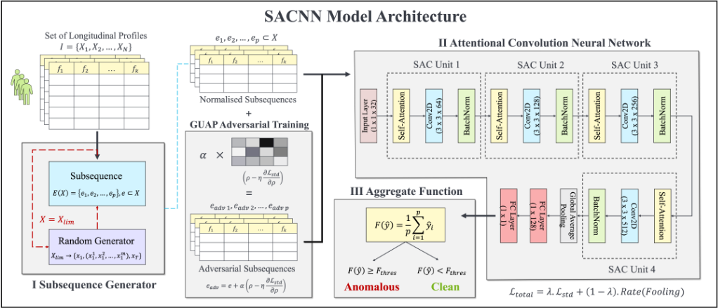
Our proposed model consists of three main components: a subsequence generator, an attentional convolution neural network, and an aggregate function together with adversarial training, as shown in Figure 1.
4.1 Subsequence Generator
Input data is a collection of sequences I = {X1,X2, ...XN} with length of the sequences n1, n2, ...nN respectively. Since each sequence is of a different length, and the model requires an input of fixed dimensions, we generate subsequences of fixed dimensions out of the given sequence. The subsequence generator performs this operation in two steps. First it scans whether the sequence is a limited sequence Xlim. In this case, it is not possible to generate the subsequences, so the random generator randomly generates m additional samples based on sample x1 within the measurement uncertainty limit of ±10% and x2 can be treated as xT . It is a standard systematical uncertainty caused by the quantification instrument taken from biochemical domain experts [WADA, 2021]. The output of the random generator is the sequence consisting of x1, m generated samples, and x2. Next, the generator encodes each sequence into a set of subsequences denoted by E(X) where p represents the total number of generated subsequences for the given sequence X as shown below:
Each subsequence e has a fixed length denoted by le and consists of e = {xi, xi+1, ..., xle-1, xT}, xi, ..., xle-1 ∈ X. In this case, we compare the similarity of xT with the other elements in the subsequence. The generator generates sequences corresponding to all the possible combinations of the elements. This step is similar to the sliding window operation. However, the main difference is in this case, we want to consider all possible combinations of the elements of the sequence with xT into account and let the model learn the spatio-temporal relationship in all the combinations. The number of subsequences p can be calculated by:
where n represents the number of elements in the sequence X, and nxT represents the number of testing samples under consideration. These subsequences are then normalised separately. Therefore, the output is a set of normalised subsequences.
4.2 Attentional Convolution Neural Network
We propose a network architecture consisting of an input layer, four SAC units and a fully connected layer.
Input Layer
The input layer is Conv1D layer with 32 filters (1 × 1 × 32). It takes subsequence ei as input to perform a convolution operation and generates low-level embeddings for the given subsequence while preserving the spatial dimension. Therefore, the output is in a tensor format χ ∈ RN1×N2×N3 , where N1,N2,N3 denote length of subsequence, number of parameters, number of filters respectively.
SAC Unit
Each unit consists of self-attention layer, 2D convolution layer and batch normalisation.
1) Self-Attention Layer: The input tensor is first flattened using the reshaping layer. This is to make sure 2D embedding sequence is fed into the attention layer.
We use the self-attention layer for two reasons. Firstly, we are interested in mapping the spatio-temporal relationships of the embedding subsequence, i.e. compare each parameter of each element with itself. The attentional weights represent this relationship and can be used to generate high-level embeddings. Secondly, it increases the receptive field of the convolutional layer without adding computational costs associated with very large filter sizes.
The self-attention layer maps a query Qi and a set of keyvalue pairs (Ki, Vi) to an output. The output is computed as a weighted sum of the values, where the weight assigned to each value is computed using the given query and the key. In our case, given the low-level embedding sequence from the input layer, the dot-product attention operation can be computed as:
The single attention layer performing h multi-head attention operation can be computed as:
where Qi = χ.wQ i , Ki = χ.wK i , Vi = χ.wV i and the learned attentional weights of the attention layer are:
The output of the attention layer consists of high-level embeddings with the same spatial dimensions, i.e. χatt ∈ RN1.N2×N3 . The reshaping layer changes back the dimension to χatt ∈ RN1×N2×N3 for the convolution layer.
2) 2D Convolution Layer: We use the convolution layer for three reasons. Firstly, it can learn the spatial relationship using filters, which is useful for this task. Secondly, it can learn more complex patterns from spatial space by stacking multiple filters. Lastly, the optimisation of the network could be efficiently performed by stochastic gradient descent algorithms on commercial hardware.
We use Conv2D layer with l filters (m×m×l) and padding to preserve the spatial dimension, where l = le. It can be represented by:
where C l i,j is lth filter which convolves over the embedding map χatt and represents the element-wise weights. Thus, the output feature map Sout i,j is obtained by different Conv2D filters:
where σ denotes the Leaky-ReLU activation function.
3) Batch Normalisation: Batch normalisation is used to reduce internal covariate shift caused by the attention and convolutional layers and for faster and more stable training.
where γ and β are learnable parameters and ˆχconv denotes normalised input to zero mean and unit variance.
Fully-Connected Layer
The output of the last SAC unit is first flattened using a global average pooling layer to χBN ∈ Rl . We use a fullyconnected layer which takes the flattened input and evaluates the probability of whether it has a fraudulent trade. If the probability is greater than the threshold value Pthres, the subsequence can be classified as anomalous.
where W denotes weight matrix and B represents bias vector. We used the cross entropy loss defined as:
where ˆ yi ∈ {0, 1} denotes the predicted label for the subsequence, and yi ∈ {0, 1} denotes the ground truth label, which is set to 1 if the subsequence is anomalous and 0 otherwise. f(χBN ) is the detection function that maps χBN to probability of whether the current subsequence is fraudulent. The proposed model can be optimised through the standard stochastic gradient descent algorithm. We used adam optimizer to learn the weights, and set the learning rate to 1e-3 and batch size to 256.
4.3 Aggregate Function
Since we get predictions ˆ yi for each subsequence separately from the fully connected layer. Therefore, we need an aggregate function to add each prediction and determine the final decision on the sequence. The aggregate function tells the likelihood of the given sequence being anomalous and can be defined as:
The final classification of the sequence can be calculated by:
where the value of Fthres is arbitrary and can be set accordingly to achieve high specificity.
4.4 Adversarial Training
We used adversarial training for two reasons. First, it adds novelty to the model by allowing it to recognise and classify variations in the input data that it may not have seen before. This can help to improve the model's generalisation capability and make it more robust to unseen profiles. Second, it is used as fairness-aware training that helps to eliminate discrimination or bias in the predictions. This can be done by incorporating fairness constraints into the training process, such as ensuring that the model's predictions are not systematically worse for certain demographic groups (e.g. based on gender, race, etc.). We employed SoTA adversarial attack called Generalised Universal Adversarial Perturbation (GUAP) [Zhang et al., 2020] to generate adversarial samples for the model. The goal of an GUAP attack is to generate single perturbations to the multiple input that cause the model to make a mistake. The generated samples can be represented as:
We used a loss function that penalises the model for producing outputs that are different from the original input. So the total loss function for the model can be represented as:
where ρ denotes the perturbation vector, α denotes perturbation constant, η represents learning rate, and λ controls the balance between the two loss functions.
5 Experiments
5.1 Datasets
We use real-world athlete datasets consisting of steroid longitudinal profiles with 11 parameters (Table 1) gathered by anti-doping agencies at various athletic events worldwide. The data is extracted from the Anti-Doping Administration & Management System (ADAMS) database [WADA, 2005] and [Rahman et al., 2022b] showed a detailed descriptive analysis of these datasets, including distributions, ranges, etc., where each dataset contains < 20% anomalous profiles, i.e., one sample is swapped in each profile (nxT = 1). In addition, the dataset Steroid-M and Steroid-F represent the case of limited longitudinal profile Xlim.
| Datasets | Athlete | Profiles | Samples | le |
|---|---|---|---|---|
| Steroid-M | Male | 755 | 4214 | 3-20 |
| Steroid-F | Female | 375 | 2307 | 3-20 |
| Steroid-M | Male | 737 | 1474 | 2 |
| Steroid-F | Female | 293 | 586 | 2 |
5.2 Baseline Methods
We employed the following SoTA models to compare the performance of our proposed model SACNN.
- Beta-VAE: [Higgins et al., 2017] Variational autoencoder uses modified reconstruction loss to find anomaly in a sequence.
- V-LSTM: [Lin et al., 2020] Sliding window based approach uses joint learning of VAE and LSTM to generate low-dimensional embeddings for anomaly detection.
- SUOD: [Zhao et al., 2021] Ensemble approach produce acceleration to different heterogeneous models for anomaly detection.
- XGBOD: [Zhao and Hryniewicki, 2018] Semisupervised boosting algorithm to extract useful embeddings from the sequence to detect outlier.
- LSCP: [Zhao et al., 2019] Unsupervised parallel ensemble algorithm which selects competent detectors in the local region of a sequential instance to detect outlier.
- AnoGAN: [Schlegl et al., 2017] Deep convolutional generative adversarial network that learns a manifold of normal anatomical variability to detect anomalies.
- IsoForest: [Liu et al., 2008] Unsupervised learning approach that constructs multiple trees which isolate observations with different characteristics to identify outliers.
5.3 Experimental Settings
We used the Steroid-All dataset [Rahman et al., 2022b] for training and validating all the models, which contains 50,450 clean profiles from both male and female athletes. In this dataset, we randomly selected 50% of profiles and manually swapped one sample in each profile with a sample from a different profile and labelled them as anomalous profiles (class 1). The other 50% of the profiles were labelled as clean profiles (class 0). Each profile is normalised separately, i.e. all the samples within the profile are normalised to the unit norm. We used 80% of the dataset for training all the models and 20% for the validation and evaluated the performance of SACNN against the baseline models. We need the model's performance at high specificity, which is a requirement from the anti-doping domain to avoid false negatives and unnecessary DNA testing (reducing unnecessary costs) and, hence, mimic the real-world situation. Therefore, we optimise the hyperparameters of all the baseline models to achieve optimal sensitivity under high specificity (99 ± 0.1)%.
6 Results
We compared the performance of SACNN with different baseline models on different datasets, as shown in Table 2. The uncertainties are evaluated using 5 fold cross-validation method. In all baselines, XGBOD and V-LSTM proven to be competitive, demonstrating the necessity of embedding extraction models for fraud detection. However, even with an accuracy of > 70%, Beta-VAE could not be able to detect any anomalous profiles (sensitivity of < 1%). In the case of limited profiles, we observe that all the models except SUOD show poor performance on Steroid-M dataset (in terms of sensitivity). However, for the Steroid-F dataset XGBOD and V-LSTM show better performance. The accuracy of all the models is much better because of the highly imbalanced nature of the datasets. Our proposed model outperforms all the baselines, i.e. generating spatio-temporal embeddings prove to be effective. SACNN achieves the sensitivity value of > 50% and AU value of > 80% on all the datasets.
6.1 Precision-Recall Curve
Figure 2 shows ROC and PRC curves for all the models evaluated on the Steroid-M dataset. As shown, the SACNN model performs better than all the baselines concerning both curves. The results of V-LSTM, SUOD and LSCP are quite similar.
| Datasets | Mtr | Beta-VAE | V-LSTM | SUOD | XGBOD | LSCP | AnoGAN | IsoForest | SACNN |
|---|---|---|---|---|---|---|---|---|---|
| Steroid-M | AC | 0.75±0.04 | 0.81±0.03 | 0.79±0.02 | 0.85±0.01 | 0.78±0.03 | 0.77±0.02 | 0.79±0.00 | 0.93±0.02 |
| SP | 0.99±0.01 | 0.99±0.01 | 0.99±0.01 | 0.99±0.01 | 0.99±0.01 | 0.99±0.01 | 0.99±0.01 | 0.99±0.01 | |
| SN | 0.01±0.01 | 0.31±0.04 | 0.20±0.04 | 0.42±0.02 | 0.13±0.05 | 0.09±0.03 | 0.30±0.01 | 0.74±0.03 | |
| AU | 0.50±0.00 | 0.75±0.03 | 0.73±0.02 | 0.79±0.00 | 0.61±0.02 | 0.60±0.01 | 0.74±0.01 | 0.92±0.01 | |
| Steroid-F | AC | 0.78±0.02 | 0.83±0.03 | 0.79±0.02 | 0.84±0.03 | 0.78±0.02 | 0.78±0.01 | 0.82±0.01 | 0.90±0.03 |
| SP | 0.99±0.01 | 0.99±0.01 | 0.99±0.01 | 0.99±0.01 | 0.99±0.01 | 0.99±0.01 | 0.99±0.01 | 0.99±0.01 | |
| SN | 0.00±0.00 | 0.38±0.05 | 0.10±0.03 | 0.40±0.04 | 0.01±0.03 | 0.00±0.00 | 0.36±0.01 | 0.65±0.03 | |
| AU | 0.50±0.01 | 0.77±0.04 | 0.65±0.01 | 0.79±0.03 | 0.53±0.01 | 0.50±0.00 | 0.78±0.01 | 0.85±0.01 | |
| Steroid-M | AC | 0.72±0.04 | 0.80±0.03 | 0.81±0.01 | 0.82±0.02 | 0.79±0.02 | 0.77±0.03 | 0.77±0.02 | 0.90±0.02 |
| SP | 0.99±0.01 | 0.99±0.01 | 0.99±0.01 | 0.99±0.01 | 0.99±0.01 | 0.99±0.01 | 0.99±0.01 | 0.99±0.01 | |
| SN | 0.02±0.01 | 0.23±0.02 | 0.34±0.04 | 0.31±0.02 | 0.29±0.01 | 0.18±0.04 | 0.28±0.01 | 0.70±0.01 | |
| AU | 0.52±0.00 | 0.78±0.01 | 0.76±0.03 | 0.77±0.00 | 0.66±0.00 | 0.60±0.02 | 0.74±0.02 | 0.90±0.00 | |
| Steroid-F | AC | 0.71±0.03 | 0.79±0.02 | 0.77±0.02 | 0.79±0.01 | 0.73±0.03 | 0.73±0.02 | 0.75±0.03 | 0.84±0.01 |
| SP | 0.99±0.01 | 0.99±0.01 | 0.99±0.01 | 0.99±0.01 | 0.99±0.01 | 0.99±0.01 | 0.99±0.01 | 0.99±0.01 | |
| SN | 0.01±0.02 | 0.47±0.04 | 0.09±0.03 | 0.50±0.00 | 0.18±0.03 | 0.14±0.03 | 0.33±0.01 | 0.52±0.00 | |
| AU | 0.51±0.00 | 0.72±0.02 | 0.54±0.01 | 0.74±0.00 | 0.61±0.02 | 0.59±0.01 | 0.70±0.01 | 0.81±0.00 |
All of them are much better than Beta-VAE. This might be because the fraud behaviour in longitudinal profiles is too complex for a simple autoencoder model to address. Among all the baselines, XGBOD is shown to be the most competitive. It might be because it generates a deep representation of parameters into embeddings using boosting algorithm.
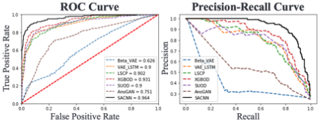
Our proposed SACNN model consistently outperforms other SoTA baseline models. The reason is: (1) it deals with both spatial and temporal behaviour and generates embedding maps using an attention network, contrasted with XGBOD, which only deals with the spatial pattern and cannot address temporal behaviour of the longitudinal profile; (2) SACNN uses a convolutional network for better pattern learning from the generated embedding maps. Our model works even better at the very beginning of the curve compared to the other baselines. Moreover, our model can accurately detect more fraud longitudinal profiles with a high specificity.
6.2 Parameter Sensitivity
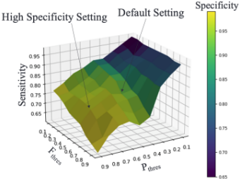
We studied the impact of different values of threshold parameters on the performance of our SACNN model. We varied both the threshold parameters (Pthres and Fthres) from 0 to 1 with a step of 0.1 and evaluated the sensitivity and specificity of the model. As shown in Figure 3, the sensitivity is dropping if we keep increasing the value of Pthres and Fthres, but it improves the specificity because of the tradeoff between the two. However, we observed that Pthres has a greater impact than Fthres because it is the threshold acting on the predictions of each subsequence individually. So, we set Pthres = 0.5 and Fthres = 0.5 as default setting and Pthres = 0.8 and Fthres = 0.6 to be high specificity setting i.e. 99% specificity value.
7 Case Study
To understand the spatio-temporal patterns of the longitudinal profile from the embedding maps, we performed a study on real-world proven cases. These longitudinal profiles were tested using DNA analysis performed by an accredited antidoping laboratory and found that 2 profiles were proven for sample swapping, 5 for doping and 22 for clean profiles. Our model could able to detect all the sample swapping and doping cases and 20/22 clean profiles. We selected one clean and one anomalous profile (sample swapping) and plotted the subsequence and the generated embedding maps from each SAC unit in Figure 4. The total number of embedding maps generated by the attention mechanism depends on the output of the Conv2D layer of the previous SAC unit. Therefore, these maps represent high-level embeddings. We plotted one of each embedding map to understand how the attentional weights in these maps are evolving. In the case of clean subsequence, we have higher weights in the embedding map of SAC unit 4 than anomalous subsequence, which shows a strong spatio-temporal relationship among three samples. Furthermore, the evolution of embedding maps also shows why we need at least 4 SAC units.

8 Ablation Studies
As shown in Table 3, we studied the effect of different components in SACNN. First, we removed the attention layer in the SAC units (w/o Att) and observed that the model's performance was degraded because the convolutional network is now learning the spatial relationship of the normalised subsequences instead of spatio-temporal embedding maps. This shows the importance of considering the spatio-temporal behaviour of the sequence. Second, we removed the adversarial attack in the model (w/o Adv) and observed that the model is less robust to the variation in input data. Next, we varied the number of SAC units in the model and observed that the model performs better when we keep adding a SAC unit until a point after which the performance starts dropping. The reason might be that adding a SAC unit helps to evolve the embedding maps, but once it is fully generated, adding more units will introduce overfitting. Moreover, adding SAC units exponentially increases the number of trainable parameters. Therefore, we selected 4 SAC units in the SACNN model.
To understand the significance of the subsequence genera- Table 3: Ablation studies showing the model performance evaluated on Steroid-M dataset at high specificity setting.
| Model | AC | SN | AU | # parameters |
|---|---|---|---|---|
| w/o Att | 0.871 | 0.505 | 0.829 | 1.6M |
| w/o Adv | 0.893 | 0.658 | 0.823 | 1.2M |
| w Mask | 0.841 | 0.418 | 0.790 | 2.0M |
| w Add Samp | 0.858 | 0.490 | 0.816 | 2.0M |
| 1 SAC | 0.860 | 0.502 | 0.815 | 50k |
| 2 SAC | 0.873 | 0.523 | 0.834 | 180k |
| 3 SAC | 0.890 | 0.642 | 0.856 | 600k |
| 5 SAC | 0.903 | 0.664 | 0.880 | 7.1M |
| SACNN | 0.926 | 0.737 | 0.916 | 2.0M |
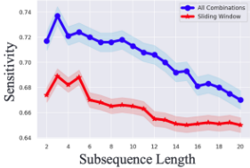
tor, we test two different variants of the model where instead of generating subsequence of length le, 1) we generate additional samples based on other samples to achieve the same length for all the sequences (w Add Samp). 2) we mask the additional samples with padding (w Mask). We observed that adding additional samples to shorter sequences will cause a bias in the model's decision since we know xT is not similar to masked or generated samples. Figure 5 shows the effect of different subsequence lengths le on the model's performance for both sliding window and our approach of considering all the combinations for defining the subsequences. We found 3 as an optimum subsequence length for our model.
9 Conclusion
In this paper, we propose an attention-based approach that takes into account the spatial and temporal behaviour of the longitudinal profile of athletes. It generates embedding maps using an attention mechanism and let the convolutional network capture the implicit relationship from these embedding maps. Our model achieves promising sensitivity at a high specificity value compared with SoTA baseline models. Furthermore, we explore the spatio-temporal patterns by observing the generated embedding maps in the case study on longitudinal profiles tested by DNA analysis. The results demonstrate that our model can effectively detect sample swapping and can help anti-doping authorities trigger fraudulent practices during sports events and make the sports clean.
@inproceedings{ijcai2024p665,
  title     = {SACNN: Self Attention-based Convolutional Neural Network for Fraudulent Behaviour Detection in Sports},
  author    = {Rahman, Maxx Richard and Abdel Khaliq, Lotfy and Piper, Thomas and Geyer, Hans and Equey, Tristan and Baume, Norbert and Aikin, Reid and Maass, Wolfgang},
  booktitle = {Proceedings of the Thirty-Third International Joint Conference on
               Artificial Intelligence, {IJCAI-24}},
  publisher = {International Joint Conferences on Artificial Intelligence Organization},
  editor    = {Kate Larson},
  pages     = {6017--6025},
  year      = {2024},
  month     = {8},
  note      = {Main Track},
  doi       = {10.24963/ijcai.2024/665},
  url       = {https://doi.org/10.24963/ijcai.2024/665},
}
TY - CPAPER TI - SACNN: Self Attention-based Convolutional Neural Network for Fraudulent Behaviour Detection in Sports AU - Rahman, Maxx Richard AU - Abdel Khaliq, Lotfy AU - Piper, Thomas AU - Geyer, Hans AU - Equey, Tristan AU - Baume, Norbert AU - Aikin, Reid AU - Maass, Wolfgang T2 - Proceedings of the Thirty-Third International Joint Conference on Artificial Intelligence, IJCAI-24 PB - International Joint Conferences on Artificial Intelligence Organization PY - 2024 SP - 6017 EP - 6025 DO - 10.24963/ijcai.2024/665 UR - https://doi.org/10.24963/ijcai.2024/665 ER -Copied
Machine-readable versions of this paper, for tools and AI agents:





