
Robust Reward Placement under Uncertainty
Proceedings of the Thirty-Third International Joint Conference on Artificial Intelligence. Main Track. Pages 6770-6778.
https://doi.org/10.24963/ijcai.2024/748
Keywords
- Planning and Scheduling: PS: Planning under uncertainty
- Search: S: Combinatorial search and optimisation
- Data Mining: DM: Networks
- Planning and Scheduling: PS: Markov decisions processes
Abstract
We consider a problem of placing generators of rewards to be collected by randomly moving agents in a network. In many settings, the precise mobility pattern may be one of several possible, based on parameters outside our control, such as weather conditions. The placement should be robust to this uncertainty, to gain a competent total reward across possible networks. To study such scenarios, we introduce the Robust Reward Placement problem (RRP). Agents move randomly by a Markovian Mobility Model with a predetermined set of locations whose connectivity is chosen adversarially from a known set Π of candidates. We aim to select a set of reward states within a budget that maximizes the minimum ratio, among all candidates in Π, of the collected total reward over the optimal collectable reward under the same candidate. We prove that RRP is NP-hard and inapproximable, and develop Ψ-Saturate, a pseudo-polynomial time algorithm that achieves an ϵ-additive approximation by exceeding the budget constraint by a factor that scales as O(ln |Π|/ϵ). In addition, we present several heuristics, most prominently one inspired by a dynamic programming algorithm for the max–min 0–1 KNAPSACK problem. We corroborate our theoretical analysis with an experimental evaluation on synthetic and real data.
- [Adiga et al., 2014] Abhijin Adiga, Chris J. Kuhlman, Hen- ning S. Mortveit, and Anil Kumar S. Vullikanti. Sensitiv- ity of diffusion dynamics to network uncertainty. J. Artif. Intell. Res., 51:207-226, 2014.
- [Aissi et al., 2009] Hassene Aissi, Cristina Bazgan, and Daniel Vanderpooten. Min-max and min-max regret ver- sions of combinatorial optimization problems: A survey. Eur. J. Oper. Res., 197(2):427-438, 2009.
- [Amelkin and Singh, 2019] Victor Amelkin and Ambuj K. Singh. Fighting opinion control in social networks via link recommendation. In ACM SIGKDD, pages 677-685, 2019.
- [Bollobás et al., 2003] Béla Bollobás, Christian Borgs, Jen- nifer T. Chayes, and Oliver Riordan. Directed scale-free graphs. In ACM-SIAM SODA, pages 132-139, 2003.
- [Brin and Page, 1998] Sergey Brin and Lawrence Page. The anatomy of a large-scale hypertextual web search engine. Computer networks and ISDN systems, 30(1-7):107-117, 1998.
- [Chen et al., 2016] Wei Chen, Tian Lin, Zihan Tan, Mingfei Zhao, and Xuren Zhou. Robust influence maximization. In ACM SIGKDD, pages 795-804, 2016.
- [Dinur and Steurer, 2014] Irit Dinur and David Steurer. An- alytical approach to parallel repetition. In ACM STOC, pages 624-633, 2014.
- [Du et al., 2013] Nan Du, Le Song, Manuel Gomez- Rodriguez, and Hongyuan Zha. Scalable influence estima- tion in continuous-time diffusion networks. In NeurIPS, pages 3147-3155, 2013.
- [Garey and Johnson, 1979] Michael R. Garey and David S. Johnson. Computers and Intractability: A Guide to the Theory of NP-Completeness. W. H. Freeman, 1979.
- [He and Kempe, 2016] Xinran He and David Kempe. Robust influence maximization. In ACM SIGKDD, pages 885- 894, 2016.
- [Horčík et al., 2022] Rostislav Horčík, Alvaro Torralba, Pavel Rytíř, Lukáš Chrpa, and Stefan Edelkamp. Opti- mal mixed strategies for cost-adversarial planning games. In Intl Conf. on Autom. Plan. and Sched., pages 160-168, 2022.
- [Ivanov et al., 2017] Sergei Ivanov, Konstantinos Theocharidis, Manolis Terrovitis, and Panagiotis Karras. Content recommendation for viral social influence. In ACM SIGIR, pages 565-574, 2017.
- [Johnson et al., 2000] David S. Johnson, Maria Minkoff, and Steven Phillips. The prize collecting Steiner tree problem: theory and practice. In ACM-SIAM SODA, pages 760-769, 2000.
- [Karp, 1972] Richard M. Karp. Reducibility among combi- natorial problems. In Complexity of Computer Computa- tions, pages 85-103, 1972.
- [Kempe et al., 2003] David Kempe, Jon M. Kleinberg, and Éva Tardos. Maximizing the spread of influence through a social network. In ACM SIGKDD, pages 137-146, 2003.
- [Kouvelis and Yu, 1997] Panos Kouvelis and Gang Yu. Ro- bust Discrete Optimization and Its Applications, vol- ume 14 of Nonconvex Optimization and Its Applications. Springer, 1997.
- [Krause and Golovin, 2014] Andreas Krause and Daniel Golovin. Submodular function maximization. In Tractability: Practical Approaches to Hard Problems, pages 71-104. Cambridge University Press, 2014.
- [Krause et al., 2008] Andreas Krause, H. Brendan McMa- han, Carlos Guestrin, and Anupam Gupta. Robust sub- modular observation selection. Journ. of Mach. Learn. Res., 9(93):2761-2801, 2008.
- [Li and Yang, 2020] Huiran Li and Yanwu Yang. Optimal keywords grouping in sponsored search advertising under uncertain environments. International Journal of Elec- tronic Commerce, 24(1):107-129, 2020.
- [Logins et al., 2020] Alvis Logins, Yuchen Li, and Panagio- tis Karras. On the robustness of cascade diffusion under node attacks. In The Web Conference, pages 2711-2717, 2020.
- [Logins et al., 2022] Alvis Logins, Yuchen Li, and Panagi- otis Karras. On the robustness of diffusion in a net- work under node attacks. IEEE Trans. Knowl. Data Eng., 34(12):5884-5895, 2022.
- [Martello and Toth, 1987] Silvano Martello and Paolo Toth. Algorithms for knapsack problems. In Surveys in Com- binatorial Optimization, volume 132 of North-Holland Mathematics Studies, pages 213-257. 1987.
- [Minoux, 1978] Michel Minoux. Accelerated greedy algo- rithms for maximizing submodular set functions. In IFIP Conference on Optimization Techniques, pages 234-243, 1978.
- Erik Ordentlich and Thomas M. Cover. The cost of achieving the best portfolio in hindsight. Math. Oper. Res., 23(4):960-982, 1998.
- [Ostachowicz et al., 2019] Wieslaw Ostachowicz, Rohan Soman, and Pawel Malinowski. Optimization of sen- sor placement for structural health monitoring: a review. Structural Health Monitoring, 18(3):963-988, 2019.
- [Petsinis et al., 2024] Petros Petsinis, Kaichen Zhang, An- dreas Pavlogiannis, Jingbo Zhou, and Panagiotis Kar- ras. Robust reward placement under uncertainty. arXiv:2405.05433, 2024.
- [Rosenfeld and Globerson, 2016] Nir Rosenfeld and Amir Globerson. Optimal tagging with Markov chain optimiza- tion. In NeurIPS, pages 1307-1315, 2016.
- [von Mises and Pollaczek-Geiringer, 1929] Richard von Mises and Hilda Pollaczek-Geiringer. Praktische ver- fahren der gleichungsauflösung. ZAMM -Zeitschrift für Angewandte Mathematik und Mechanik, 9(1):58-77, 1929.
- [Wolsey, 1982] Laurence A. Wolsey. An analysis of the greedy algorithm for the submodular set covering prob- lem. Combinatorica, 2(4):385-393, 1982.
- [Yu, 1996] Gang Yu. On the max-min 0-1 knapsack prob- lem with robust optimization applications. Operations Re- search, 44(2):407-415, 1996.
- [Zhang and Vorobeychik, 2016] Haifeng Zhang and Yev- geniy Vorobeychik. Submodular optimization with routing constraints. In AAAI Conf. on Artif. Intell., pages 819-826, 2016.
- [Zhang et al., 2020] Kaichen Zhang, Jingbo Zhou, Donglai Tao, Panagiotis Karras, Qing Li, and Hui Xiong. Geode- mographic influence maximization. In ACM SIGKDD, pages 2764-2774, 2020.
References were extracted automatically from the PDF and may contain errors.
Full text extracted automatically from the PDF; figures, tables and equations may differ. The PDF is the version of record.
1 Introduction
In many graph optimization problems, a stakeholder has to select locations in a network, such as a road, transportation, infrastructure, communication, or web network, where to place reward-generating facilities such as stores, ads, sensors, or utilities to best service a population of moving agents such as customers, autonomous vehicles, or bots [Zhang and Vorobeychik, 2016; Ostachowicz et al., 2019; Zhang et al., 2020; Rosenfeld and Globerson, 2016; Amelkin and Singh, 2019]. Such problems are intricate due to the uncertainty surrounding agent mobility [Krause et al., 2008; Chen et al., 2016; He and Kempe, 2016; Horˇc´ık et al., 2022].
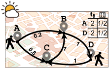
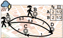
For instance, consider outdoor ad placement. We represent the road map as a probabilistic network in which agents move. If every agent follows the same movement pattern regardless of environmental conditions, then the problem of placing ads to maximize the expected number of ad views admits a greedy algorithm with an approximation ratio [Zhang et al., 2020]. Still, the problem becomes more involved under malleable environmental conditions that alter movement patterns. As a toy example, Figure 1 shows a probabilistic network. An agent randomly starts from an initial location and takes two steps by the probabilities shown on edges representing street segments, under two environmental settings, sunny and rainy. Assume a stakeholder has a budget to place an ad-billboard at a single location. Under the sunny setting, the best choice of placement is B, as the agent certainly passes by that point regardless of its starting position; under the rainy setting, the agent necessarily passes by D within two steps, hence that is most preferable. However, under the rainy setting B yields expected reward 0.6, and so does D under the sunny one. Due to such uncertainty, a risk-averse stakeholder would prefer the location that yields, in the worst case, the highest ratio of the collected to best feasible reward, i.e., in this case, C, which yields expected reward 0.9 under both settings.
In this paper, we introduce the problem of robust reward placement (RRP) in a network, under uncertainty about the environment whereby an agent is moving according to any of several probabilistic mobility settings. We express each such setting by a Markov Mobility Model (MMM) π ∈ Π. The cumulative reward a stakeholder receives grows whenever the agent passes by one of the reward states SR. RRP seeks to select a set of such states S ∗R within a budget, that maximizes the worst-case ratio, across all settings Π, of the collected reward F(SR|π) over the highest reward that can be collected under the same setting F(S ∗ π |π), i.e., S ∗R = argmaxSR minπ∈Π F (SR|π) F (S ∗ π |π) . This max-min ratio objective is used in risk-averse portfolio optimization and advertising [Ordentlich and Cover, 1998; Li and Yang, 2020].
Our Contribution. Our contributions stand as follows:
- We introduce the problem of Robust Reward Placement (RRP) over a set of Markov Mobility Models, that has real-world applications across various domains.
- We study the properties of RRP and show that it is NPhard (Theorem 1). Due to the additivity and monotonicity properties of the reward function (Lemma 3), it admits an optimal solution in pseudo-polynomial time under a single setting, i.e. |Π| = 1 (Lemma 4), yet it is inapproximable when |Π| > 1 unless we exceed the budget constraint by a factor O(ln |Π|) (Theorem 2).
- We adopt techniques from robust influence maximization to develop Ψ-Saturate, a pseudo-polynomial time algorithm that finds a solution within ϵ distance of the optimal, i.e. OPT - ϵ, while exceeding the budget constraint by an O(ln |Π|/ϵ) factor (Lemma 6).
- We present several heuristics as alternative solutions, most prominently one based on a dynamic programming algorithm for the max-min 0-1 KNAPSACK problem, to which RRP can be reduced (Lemma 5).
We corroborate our analysis with an experimental evaluation on synthetic and real data. Due to space constraints, we relegate some proofs to the full version [Petsinis et al., 2024].
2 RelatedWork
The Robust Reward Placement problem relates to robust maximization of spread in a network, with some distinctive characteristics. Some works [Du et al., 2013; He and Kempe, 2016; Chen et al., 2016; Logins et al., 2020; Logins et al., 2022] study problems of selecting a seed set of nodes that robustly maximize the expected spread of a diffusion process over a network. However, in those models [Kempe et al., 2003] the diffusion process is generative, whereby an item propagates in the network by producing unlimited replicas of itself. On the other hand, we study a non-generative spread function, whereby the goal is to reach as many as possible out of a population of network-resident agents. Our spread function is similar to the one studied in the problem of Geodemographic Influence Maximization [Zhang et al., 2020], yet thereby the goal is to select a set of network locations that achieves high spread over a mobile population under a single environmental setting. We study the more challenging problem of achieving competitive spread in the worst case under uncertainty regarding the environment.
Several robust discrete optimization problems [Kouvelis and Yu, 1997] address uncertainty in decision-making by optimizing a max-min or min-max function under constraints. The robust MINIMUM STEINER TREE problem [Johnson et al., 2000] seeks to minimize the worst-case cost of a tree that spans a graph; the min-max and min-max regret versions of the KNAPSACK problem [Aissi et al., 2009] have a modular function as a budget constraint; other works examine the robust version of submodular functions [Krause and Golovin,
2014; He and Kempe, 2016] that describe several diffusion processes [Adiga et al., 2014; Krause et al., 2008]. To our knowledge, no prior work considers the objective of maximizing the worst-case ratio of an additive function over its optimal value subject to a knapsack budget constraint.
3 Preliminaries
Markov Mobility Model (MMM). We denote a discretetime MMM as π = (S, I, T ,M), where S is a set of n states, I is a vector of n elements in [0, 1] expressing an initial probability distribution over states in S, T is an n × n right-stochastic matrix, where T [s, s′ ] is the probability of transition from state s ∈ S to another state s′ ∈ S, and M is an n × K matrix with elements in [0, 1], where K is the maximum number of steps andM[s, k] expresses the cumulative probability that an agent starting from state s ∈ S takes k′ ∈ [k,K] steps. Remarkably, an MMM describes multiple agents and movements, whose starting positions are expressed via initial distribution I and their step-sizes viaM.
Rewards. Given anMMM, we select a set of states to be reward states. We use a reward vector R ∈ {0, 1}n to indicate whether state s ∈ S is a reward state and denote the set of reward states as SR = {s ∈ S|R[s] = 1}. In each timestamp t, an agent at state s moves to state s′ and retrieves reward R[s′ ]. For a set of reward states SR, and a given MMM π, the cumulative reward F(SR|π) of an agent equals:
where Fπ(SR|k) is the expected reward at the kth step, Mk is the kth column of M, and ◦ denotes the Hadamard product. Connection to Pagerank. The Pagerank algorithm [Brin and Page, 1998], widely used in recommendation systems, computes the stationary probability distribution of a random walker in a network. The Pagerank scores are efficiently computed via power-iteration method [von Mises and PollaczekGeiringer, 1929]. Let PR be an N × 1 column-vector of the Pagerank probability scores, initialized as PR(0), T is an N × N matrix featuring the transition probabilities of walker, and 1 be the all-ones vector. For a damping factor a, the power method computes the scores in iterations as:
We repeat this process until convergence, i.e., until |PR(t)- PR(t - 1)| ≤ ϵ for a small ϵ ≥ 0. We denote the PageRank score at the ith node as PR[i]. For a sufficiently large number of steps K for each state with Mk = 1∀k ∈ [K], Equation (2) becomes Fπ(k) = R⊤ (T k I ). Likewise, for damping factor a = 1, Equation (3) becomes PR(t) = TtPR(0), thus the two equations are rendered analogous with T = T and PR(0) = I. Then, considering that the iteration converges from step ˆ k onward, the expected reward from reward state si per step k ≥ ˆ k, Fπ({si}|k), is the PageRank score of the ith node, that is PR[i]. To see this, let Ri = 1i be the reward vector when si ∈ S is the only reward state; then it holds that PR[i] = 1⊤i (TkPR(0)) =R⊤i (T k I ) = Fπ({si}|k).
4 ProblemFormulation
In this section we model the uncertain environment where individuals navigate and introduce the Robust Reward Placement (RRP) problem over a set of Markov Mobility Models (MMMs), extracted from real movement data, that express the behavior of individuals under different settings.
Setting. Many applications generate data on the point-topoint movements of agents over a network, along with a distribution and their total number of steps. Using aggregate statistics on this information, we formulate, without loss of generality, the movement of a population by a single agent moving probabilistically over the states of an MMM π = (S, I, T ,M). Due to environment uncertainty, the agent may follow any of |Π| different settings 1 Π = {π1, π2, . . . , π|Π|}.
Robust Reward Placement Problem. Several resource allocation problems can be formulated as optimization problems over an MMM π, where reward states SR correspond to the placement of resources. Given a budget L and a cost function c : S → N+ , the Reward Placement (RP) problem seeks a set of reward states S ∗R ⊆ S that maximizes the cumulative reward F(S ∗R|π) obtained by an agent, that is:
However, in reality the agent's movements follow an unknown distribution sampled from a set of settings Π = {π1, π2, . . . , π|Π|} represented as different MMMs. Under this uncertainty, the Robust Reward Placement (RRP) problem seeks a set of reward states SR, within a budget, that maximizes the worst-case ratio of agent's cumulative reward over the optimal one, when the model π ∈ Π is unknown. Formally, we seek a reward placement S ∗R ⊆ S such that:
where S ∗ π = argmax SR F(SR|π) is the optimal reward placement for a given model π ∈ Π within budget L. This formulation is equivalent to minimizing the maximum regret ratio of F(SR|π), i.e., 1- F(SR|π) F (S ∗ π |π) . The motivation arises from the fact that stakeholders are prone to compare what they achieve with what they could optimally achieve. The solution may also be seen as the optimal placement when the model π ∈ Π in which agents are moving is chosen by an omniscient adversary, i.e. an adversary who chooses the setting π after observing the set of reward states SR.
5 Hardness and Inapproximability Results
In this section we examine the optimization problem of RRP and we show that is NP-hard in general. First, in Theorem 1 we prove that even for a single model (|Π| = 1) the optimal solution cannot be found in polynomial time, due to a reduction from the 0-1 KNAPSACK problem [Karp, 1972].
Theorem 1. The RRP problem is NP-hard even for a single model, that is |Π| = 1.
1 We use the terms 'setting' and 'model' interchangeably.
Proof. In the 0-1 KNAPSACK problem [Karp, 1972] we are given a set of items U, each item u ∈ U having a cost c(u) and, wlog, an integer value F(u) and seek a subset V ⊆ U that has total cost ∑v∈V c(v) no more than a given budget L and maximum total value ∑v∈V F(v). In order to reduce 0-1 KNAPSACK to RRP, we set a distinct state s ∈ S for each item u ∈ U with the same cost, i.e., S = U, assign to each state a self-loop with transition probability 1, let each state be a reward state, and set a uniform initial distribution of agents over states equal to 1/|S| and steps probability equal toM[s, k] = 1, ∀k ∈ [1, . . . , F(u)]. For a single setting, an optimal solution to the RRP problem of Equation (4) is also optimal for the NP-hard 0-1 KNAPSACK problem.
Theorem 2 proves that RRP is inapproximable in polynomial time within constant factor, by a reduction from the HITTING SET problem, unless we exceed the budget constraint.
Theorem 2. Given a budget L and set of models Π, it is NPhard to approximate the optimal solution to RRP within a factor of Ω(1/n1-ϵ ), for any constant ϵ > 0, unless the cost of the solution is at least βL, with β ≥ ln |Π|.
Proof. We reduce the HITTING SET problem [Karp, 1972] to RRP and show that an approximation algorithm for RRP implies one for HITTING SET. In the HITTING SET problem, given a collection of X items, C = {c1, c2, . . . , cX} and a set of M subsets thereof, Bi ⊆ C, i ∈ {1, . . . ,M}, we seek a hitting set C ′ ⊆ C such that Bi ∩C ′ ̸= ∅ ∀i ∈ {1, . . . ,M}.
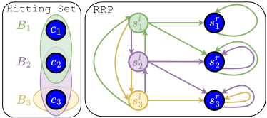
Given an instance of HITTING SET, we reduce it to RRP as follows. For each subset Bi we set a state sli ∈ S l and for each item ci we set a state sri ∈ S r . Aslo, for each subset Bi we set an MMM πi (|Π| = M) over the same set of states S = S l ∪ S r with S l ∩ S r = ∅. We set the initial probabilities I as uniform for all states in S l , equal to 1/|S l | for all models. Each model πi ∈ Π features transition probabilities 1 from each state slj to state sli , with i ̸= j, and uniform transition probabilities from sli to each state srj if and only if cj ∈ Bi. States in S r are absorbing, i.e., each state has a self-loop with probability 1. Figure 2 shows a small example of a HITTING SET instance and its RRP equivalent. We set the cost for absorbing states in S r to 1 and let each node in S l have a cost exceeding L. By this construction, if the reward placement SR does not form a hitting set, then there exists at least one subset Bi, such that Bi ∩ SR = ∅, hence minπ F (SR|π) F (S ∗ π |π) = 0. In reverse, if SR forms a hitting set, it holds that minπ F (SR|π) F (S ∗ π |π) ≥ 1 |S r | > 0. Thus, a hitting set exists if and only if minπ F (SR|π) F (S ∗ π |π) > 0. In effect, if we obtained an approximation algorithm for RRP by increasing the budget to βL, for β > 1, then we would also approximate, with a budget increased by a factor of β, the HITTING SET problem, which is NP-hard for β < (1 - δ) ln |Π| and δ > 0 [Dinur and Steurer, 2014].
6 Connections to Knapsack Problems
In this section, we establish connections between RRP and KNAPSACK problems, which are useful in our solutions.
Monotonicity and Additivity. Lemma 3 establishes that the cumulative reward function F(SR|π) is monotone and additive with respect to SR. These properties are vital in evaluating F (SR|π) while exploiting pre-computations.
Lemma 3. The cumulative reward F(SR|π) in Equation (1) is a monotone and additive function of reward states SR.
Proof. By Equation (1) we obtain the monotonicity property of the cumulative reward function F(·|π). Given a model π ∈ Π and two sets of reward states A ⊆ B ⊆ S every term of F(A|π) is no less than its corresponding term of F(B|π) due to Equation (2). For the additivity property it suffices to show that any two sets of reward states A, B ⊆ S satisfy:
Assume w.l.o.g. that the equality holds at time t, i.e. rtA + rtB = rtA∩B +rtA∪B , rtX being the cumulative reward at time t for reward states X. It suffices to prove that the additivity property holds for t + 1. At timestamp t + 1, the agent at state s ∈ S moves to s′ ∈ S. We distinguish cases as follows:
- If s′ /∈ A∪B then s′ /∈ A∩B, s′ /∈ A and s′ /∈ B, thus additivity holds.
- If s′ ∈ A ∪ B and s′ /∈ A ∩ B then either s′ ∈ A or s′ ∈ B. Assume wlog that s′ ∈ A, then it holds that: rt+1 A = rtA + T [s, s′ ], rt+1 A∪B = rtA∪B + T [s, s′ ], rt+1 B = rtB and rt+1 A∩B = rtA∩B .
- If s′ ∈ A ∩ B then s′ ∈ A and s′ ∈ B. Then, it holds that: rt+1 A = rtA +T [s, s′ ], rt+1 B = rtB +T [s, s′ ], rt+1 A∪B = rtA∪B + T [s, s′ ], and rt+1 A∩B = rtA∩B +T [s, s′ ]. In all cases the cumulative reward function is additive.
Next, Lemma 4 states that RRP under a single model π (|Π| = 1), i.e., the maximization of F(SR|π) within a budget L, is solved in pseudo-polynomial time thanks to the additivity property in Lemma 3 and a reduction from the 0-1 KNAPSACK problem [Karp, 1972]. Lemma 4 also implies that we can find the optimal reward placement with the maximum expected reward by using a single expected setting π.
Lemma 4. For a single model π (|Π| = 1) and a budget L, there is an optimal solution for RRP that runs in pseudopolynomial time O(Ln).
Proof. For each state si ∈ S we set an item ui ∈ U with cost c(ui) = c[si] and value F(ui) = F({si}|π). Since the reward function is additive (Lemma 3), it holds that F(SR|π) = ∑si∈SR F({si}|π) = ∑ui∈U F(ui). Thus, we can optimally solve single setting RRP in pseudo-polynomial time by using the dynamic programming solution for 0-1 KNAPSACK [Martello and Toth, 1987].
In the MAX-MIN 0-1 KNAPSACK problem (MNK), given a set of items U, each item u ∈ U having a cost c(u), and a collection of scenarios X, each scenario x ∈ X having a value Fx(u), we aim to determine a subset V ⊆ U, with total cost no more than L, and maximizes the minimum total value across scenarios, i.e., argV maxminx ∑u∈V Fx(u). The following lemma reduces the RRP problem to MAX-MIN 0-1 KNAPSACK [Yu, 1996] in pseudo-polynomial time.
Lemma 5. RRP is reducible to MAX-MIN 0-1 KNAPSACK in O(|Π|Ln) time.
7 Approximation Algorithm
Here, we introduce Ψ-Saturate, 2 a pseudo-polynomial time binary-search algorithm based on the Greedy-Saturate method [He and Kempe, 2016]. For any ϵ > 0, Ψ-Saturate returns an ϵ-additive approximation of the optimal solution by exceeding the budget constraint by a factor O(ln |Π|/ϵ).
Algorithm 1 Ψ-Saturate Algorithm
Input: MMMs Π, steps K, budget L, precision ϵ, param. β.
Output: Reward Placement S ∗R of cost at most βL. 1: for π ∈ Π do 2: S ∗ π ← Knapsack(π, L) 3: end for 4: ηmin ← 0, ηmax ← 1, S ∗R ← ∅ 5: while (ηmin - ηmax) ≥ ϵ do 6: η ← (ηmax + ηmin)/2 7: SR ← ∅ 8: while ∑ π∈Π min (η, F(SR|π) F (S ∗ π |π) ) < (η · |Π| - η · ϵ/3) do 9: s ← argmax s∈S\SR ∑ π∈Π 1 c(s) ( min (η, F(SR∪{s}|π) F (S ∗ π |π) ) - min (η, F(SR|π) F (S ∗ π |π) ) ) 10: SR ← SR ∪ {s} 11: end while 12: if ∑s∈SR c[s] > βL then 13: ηmax ← η 14: else 15: ηmin ← η · (1 - ϵ/3) 16: S ∗R ← SR 17: end if 18: end while 19: return S ∗RThe Ψ-Saturate Algorithm. Algorithm 1 presents the pseudocode of Ψ-Saturate. As a first step, in Lines 1-2, the algorithm finds the optimal reward placement S ∗ π for each model π ∈ Π; this is needed for evaluating the denominator of the RRP objective value in Equation (4). By Lemma 4, S ∗ π is computed in pseudo-polynomial time using the dynamic programming algorithm for the KNAPSACK problem. Then, in Lines 5-18 the algorithm executes a binary search in the range of the min-max objective ratio (Line 4). In each iteration, the algorithm makes a guess η of the optimal min-max objective value (Line 6), and then seek a set of reward states SR (Line 7), of minimum cost, with score at least η (Line 8), within distance ϵ > 0. Finding SR of the minimum cost, implies an optimal solution for the NP-hard RRP problem. Thus, in Lines 9-10, Ψ-Saturate approximates this solution by using the Greedy algorithm in [Wolsey, 1982] for function min (η, F(SR|π) F (S ∗ π |π) ) which, for fixed π and η, is monotone and submodular. 3 If the formed solution exceeds the budget constraint, the algorithm decreases the upper bound of the search scope (Lines 12-13), otherwise it increases the lower bound and updates the optimal solution S ∗R (Lines 14-16). Finally, it returns the optimal solution found (Line 19).
2 Ψ for 'pseudo-', fromGreek 'ψευδής'.
In Lemma 6 we prove that by setting β = 1 + ln 3|Π| ϵ , Ψ-Saturate approximates the optimal value within distance ϵ.
Lemma 6. For any constant ϵ > 0, let β = 1 + ln 3|Π| ϵ . Ψ-Saturate finds a reward placement SR of cost at most βL with minπ F (SR|π) F (S ∗ π |π) ≥ minπ F (S ∗R|π) F (S ∗ π |π) - ϵ = OPT - ϵ, and S ∗R = argSR maxminπ F (SR|π) F (S ∗ π |π) s.t. ∑s∈SR c[s] ≤ L.
Proof. We seek to solve a max-min regret optimization problem of an additive function under a knapsack constraint. While finding the optimal score in the denominator of the max-min ratio is NP-hard due to Theorem 1, in Line 2 we evaluate it by a pseudo-polynomial time Knapsack algorithm, as Lemma 4 allows. In Lines 5-18, we perform a binary search to find a reward placement of cost at most βL. By the analysis in [He and Kempe, 2016], the Ψ-Saturate algorithm provides an (β, OPT - ϵ) bicriteria approximation for RRP, where OPT is the optimal objective ratio score.
Unlike the pseudo-polynomial-time dynamic programming algorithm (Knapsack, Line 2) we employ, the GreedySaturate algorithm [He and Kempe, 2016] uses the Greedy 4 algorithm to approximate the optimal reward placement S ∗ π (Lines 1-2), which provides an 1/2-approximation of the optimal solution for a monotone additive function over a knapsack constraint [Garey and Johnson, 1979]. As our reward function is monotone and additive (Lemma 3), GreedySaturate offers an ( 1 2 OPT - ϵ, βL) bicriteria approximation.
Notably, for β = 1, Ψ-Saturate returns an non-constant approximation of the optimal solution within the budget constraint L. In particular, the next corollary holds.
Corollary 7. For any constant ϵ > 0, let γ = 1+ln 3|Π| ϵ . For β = 1, Ψ-Saturate satisfies the budget constraint and returns an 1 γ (OPT ′-ϵ) approximation factor of the optimal solution, with OPT ′ = maxSR minπ F (SR|π) F (S ∗ π |π) s.t. ∑s∈SR c[s] ≤ Lγ .
We stress that the approximation in Corollary 7 is nonconstant and can be arbitrarily small, as implied by the inapproximability result of Theorem 2.
3 The minimum of a constant function (η) and a monotone additive function ( F(SR|π) F(S∗π|π) , Lemma 3) is monotone and submodular. The term F(S ∗ π|π) is constant as it has been computed in Line 2.
4 The algorithm iteratively selects the element, within the budget, that offers the maximal marginal gain divided by its cost.
8 Heuristic Solutions
Inspired from previous works on node selection in networks [He and Kempe, 2016; Zhang et al., 2020] and the connection of RRP with Knapsack problems, we propose four heuristic methods. For a single model (|Π| = 1) and under uniform costs (c[s] = c ∀s ∈ S), these four heuristics find an optimal solution. However, contrary to Ψ-Saturate algorithm (Lemma 6), they may perform arbitrarily badly in the general multi-model case, even by exceeding the budget constraint. To accelerate the selection process, we use the Lazy Greedy technique that updates values selectively [Minoux, 1978] in all heuristics, except the one using dynamic programming.
All Greedy. The All Greedy method optimally solves the RRP problem for each model π ∈ Π separately using the Knapsack dynamic programming algorithm (Lemma 4) and then picks, among the collected solutions, the one yielding the best value of the objective in Equation (4). All Greedy is optimal for a single model with an arbitrary cost function.
Myopic. A greedy algorithm that iteratively chooses the reward state s∗ ∈ S, within the budget, that offers the maximal marginal gain ratio to the RRP objective divided by the cost, that is s∗ = argmax min π∈Π ( 1 c[s] F (SR∪{s}|π)-F (SR|π) F (S ∗ π |π) ).
Best-Worst Search (BWS). This algorithm uses as a score the minimum, over settings, cumulative reward for a set SR, that is H(SR) = minπ F(SR|π) and iteratively chooses the reward state s∗ ∈ S, within the budget, that offers the maximal marginal gain to that score divided by the cost, that is s∗ = argmax ( H(SR∪{s})-H(SR) c[s] ).
Dynamic Programming (DP-RRP). In Lemma 5 we reduced RRP to MAX-MIN 0-1 KNAPSACK (MNK) in pseudo-polynomial time. While MNK admits an optimal solution using a pseudo-polynomial time dynamic programming algorithm, its running time grows exponentially with the number of settings |Π| [Yu, 1996]. To overcome this time overhead, we propose a more efficient albeit non-optimal dynamic-programming algorithm for the RRP problem, noted as DP-RRP. For reward placement SR, we denote the cumulative reward for each setting as the following |Π|-tuple: g(SR) = (F(SR|π1), F(SR|π2), . . . , F(SR|π|Π|)). We use an (n + 1) × (L + 1) matrix M whose entries are |Π|- tuples of the form g(·). Let ming(SR) = minπi F(SR|πi) be the minimum reward, across |Π| settings. We define the maximum of two entries g(SR1 ) and g(SR2 ), as argmaxSR∈{SR1 ,SR2 }ming(SR), i.e. the one holding the largest minimum reward. We initialize M[·, 0] = M[0, ·] = (0, 0, . . . , 0) and recursively compute M[i, j] as follows:
where M[i, j] stands for a solution using the first i states, by some arbitrary order, and j units of budget. In the recursion of Equation (5), the first option stands for not choosing state si as a reward state, while the latter option stands for doing so while paying cost c[i] and gaining the additive reward g({i}). We compute M[n,L] as above in space and time complexity Θ(|Π|Ln) and backtrack over M to retrieve the selected reward states in the final solution. Note that, for a single model, i.e. |Π| = 1 and arbitrary cost function, Equation (5) returns an optimal solution.
Worst-case performance. While all heuristics 5 approach the optimal solution under a single setting, they may perform arbitrarily badlywithmultiple settings. In Lemma 8we prove that this holds even when exceeding the budget constraint, contrariwise to the Ψ-Saturate algorithm (Lemma 6).
Lemma 8. The heuristics for RRP may perform arbitrarily badly even when they exceed the budget constraint from L to βL, with β = 1 + ln 3|Π| ϵ and ϵ > 0.
9 Experimental Analysis
In this section we evaluate the running time and performance of algorithms on synthetic and real-world data. We use different problem parameters as Table 1 shows, marking the default value of each parameter in bold. To satisfy the budget constraint for the Ψ-Saturate algorithm, we fix β = 1 as in Corollary 7 and set precision to ϵ = (|Π| · 10 3 )-1 . We set the budget L as a percentage of the total cost ∑s∈S c[s]. To benefit from the additivity property of Lemma 3, we precompute the cumulative reward F({s}|π) for each state s ∈ S and model π ∈ Π. We implemented 6 all methods in C++ 17 and ran experiments on a 376GB server with 96 CPUs @2.6GHz.
| Parameter | Values |
|---|---|
| n | 2500, 5000, 7500, 10000, 12500 |
| ⟨d⟩ | 3,6,9,12 |
| pβ | 0.6, 0.7, 0.8, 0.9 |
| |Π| | 2,5,10,15,20 |
| K | 2,4,6,8,10 |
| L | 10%, 25%, 50%, 75% |
9.1 Synthetic Data
We use two different types of synthetic datasets to represent stochastic networks (i.e., MMMs). In each type, we generate a directed graph and then sample edge weights from a normal distribution to create different settings. In more detail:
Erd˝os-R´enyi: We generate 20 directed graphs for each of the 5 sizes shown in Table 1. In all cases, we set the edge creation probability to achieve the desired average in-degree ⟨d⟩.
Scale-Free: We generate 20 directed scale-free graphs for each of the 5 sizes shown in Table 1. Following [Bollob´as et al., 2003], we use three parameters to construct the network: pα (pγ), the probability to add a new node connected to an existing one chosen randomly by its in-degree (outdegree), and pβ, the probability to add an edge (u, v), with u and v selected by their out-degree and in-degree respectively. In all datasets, we tune pβ and set pγ = 1-pβ 3 and pα = 2pγ, so that pα + pβ + pγ = 1.
5 All algorithms work, without modification, with rewards of arbitrary non-negative values and when a partial solution is given.
6 https://anonymous.4open.science/r/RRP-F6CA
Given a graph structure, we generate |Π| = 20 distinct settings, corresponding to different models. For each setting πi, we sample the weight of edge (u, v) from a normal distribution with mean µ = 1/du and standard deviation σi = i/10du. When we sample a negative value, we set the edge weight to zero. In each resulting directed graph, we set transition probabilities T as normalized edge weights. Moreover, we set the initial probabilities I proportionally to the sum of nodes' outgoing weights and the cost of a node as the rounded-down average number of its in-neighbors among settings.
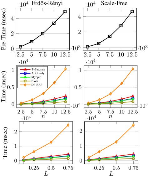
Time efficiency. Figure 3 plots the average (over 20 graphs) preprocessing time vs. graph size and running time for all algorithms vs. graph size and budget. Notably, the precomputation takes time superlinear in graph size n, as the time complexity needed for the power iteration is O(K(n +m)) for K steps maximum and m edges. The runtime of most algorithms grows linearly with graph size and budget, indicating their efficiency, except of DP-RRP, whose time complexity is at least quadratic in n, Θ(|Π|Ln) while L = Ω(n).
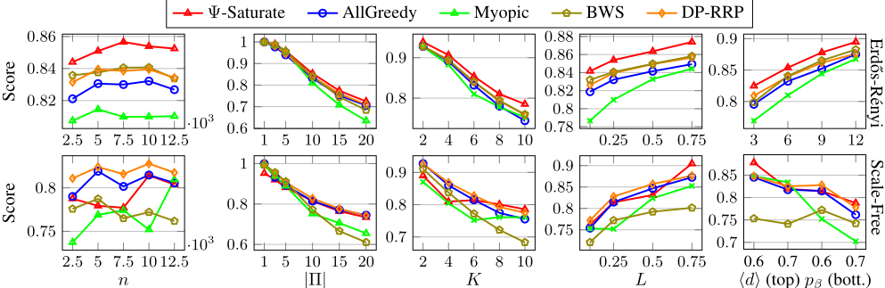
Reward placement robustness. Figure 4 illustrates the algorithms' average performance (over 20 graphs) in the reward placement robustness objective as several parameters vary. On the Erd˝os-R´enyi data, Ψ-Saturate outperforms all heuristics vs. graph size n and in other measurements, while on Scale-Free data, DP-RRP performs best overall. With a single setting, i.e., when |Π| = 1, all heuristics find an almost optimal solution. However, as expected, performance decreases as the number of models |Π| grows, whence the adversary possesses a larger pool of models to select from. Similarly, as the number of steps K grows, the feasible agent movements expand, causing the optimal cumulative reward per setting to rise more than the worst-case reward in general, hence the robustness score falls. In contrast, the score of all algorithms rises with budget L. Intuitively, a higher budget offers more flexibility to hedge against worst-case outcomes, hence better robustness scores. This effect is more evident on the Scale-Free dataset, which has fewer lucrative nodes of high in-degree. The growth of robustness scores vs. ⟨d⟩ on Erd˝os-R´enyi data confirms the importance of in-degree. On the other hand, the growth of pβ results in Scale-Free networks with more skewed power-law in-degree distributions, on which robustness scores suffer.
9.2 Real Data
To further validate our observations, we create graphs using real-world movement data. We gathered movement records fromBaiduMap, covering Xuanwu District in Nanjing 7 from July 2019 to September 2019; these records comprise sequential Points of Interest (POIs) with timestamps, allowing us to calculate the probability of transitioning between POIs based on the Markovian assumption. Using these probabilities, we construct graphs where nodes represent POIs and edges express transition probabilities. Each graph captures a 7-day period, resulting in a total of 13 graphs. The combined dataset features a total of 51943 different nodes. Out of practical considerations, we assign data-driven costs to POIs based on their visit frequency and a fixed value: c[x] = ⌊frequency(x)/25 + 50⌋. The initial and steps probabilities follow the same default setup as the synthetic datasets.
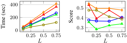
Time and Performance. Preprecessing the Xuanwu dataset where n = 51943 and |Π| = 13 takes 118 seconds. Figure 5 shows how the running time and robustness scores vary as the budget grows. DP-RRP is the most timeconsuming, followed by Ψ-Saturate, while BWS emerges as the most time-efficient solution. Interestingly, the robustness score does not follow a clear upward trend vs. budget with these real-world data; after all, the objective of Equation (4) is not a monotonic function of budget; while a higher budget allows for more flexibility in allocating resources, it also allows the optimal reward to grow correspondingly. Nevertheless, DP-RRP consistently outperforms all algorithms across budget values, corroborating its capacity to uncover high quality solutions even in hard scenarios, even while the performance of Ψ-Saturate and other heuristics fluctuates.
7 https://en.wikipedia.org/wiki/Nanjing
10 Conclusions
We introduced the NP-hard problem of Robust Reward Placement (RRP). Assuming an agent is moving on an unknown Markov Mobility Model (MMM), sampled by a set of Π candidates, RRP calls to select reward states within a budget that maximize the worst-case ratio of the expected reward (agent visits) over the optimal one. Having shown that RRP is strongly inapproximable, we propose Ψ-Saturate, an algorithm that achieves an ϵ-additive approximation by exceeding the budget constraint by a factor of O(ln |Π|/ϵ). We also developed heuristics, most saliently one based on a dynamic programming algorithm. Our experimental analysis on both synthetic and real-world data indicates the effectiveness of Ψ-Saturate and the dynamic-programming-based solution. In the future, we aim to examine the robust configuration of agent-based content features [Ivanov et al., 2017] under a set of adversarial mobility models.
Acknowledgments
Work supported by grants from DFF (P.P. and P.K., 904100382B) and Villum Fonden (A.P., VIL42117).
@inproceedings{ijcai2024p748,
  title     = {Robust Reward Placement under Uncertainty},
  author    = {Petsinis, Petros and Zhang, Kaichen and Pavlogiannis, Andreas and Zhou, Jingbo and Karras, Panagiotis},
  booktitle = {Proceedings of the Thirty-Third International Joint Conference on
               Artificial Intelligence, {IJCAI-24}},
  publisher = {International Joint Conferences on Artificial Intelligence Organization},
  editor    = {Kate Larson},
  pages     = {6770--6778},
  year      = {2024},
  month     = {8},
  note      = {Main Track},
  doi       = {10.24963/ijcai.2024/748},
  url       = {https://doi.org/10.24963/ijcai.2024/748},
}
TY - CPAPER TI - Robust Reward Placement under Uncertainty AU - Petsinis, Petros AU - Zhang, Kaichen AU - Pavlogiannis, Andreas AU - Zhou, Jingbo AU - Karras, Panagiotis T2 - Proceedings of the Thirty-Third International Joint Conference on Artificial Intelligence, IJCAI-24 PB - International Joint Conferences on Artificial Intelligence Organization PY - 2024 SP - 6770 EP - 6778 DO - 10.24963/ijcai.2024/748 UR - https://doi.org/10.24963/ijcai.2024/748 ER -Copied
Machine-readable versions of this paper, for tools and AI agents:





