
Scalable Landmark Hub Labeling for Optimal and Bounded Suboptimal Pathfinding
Proceedings of the Thirty-Third International Joint Conference on Artificial Intelligence. Main Track. Pages 6788-6795.
https://doi.org/10.24963/ijcai.2024/750
Keywords
- Search: S: Applications
- Multidisciplinary Topics and Applications: MTA: Transportation
- Planning and Scheduling: PS: Routing
- Search: S: Combinatorial search and optimisation
Abstract
Hub Labeling and A* are two well-established algorithms for shortest path computation in large graphs. Hub Labeling offers excellent query times for distance computation, but at the cost of a high space consumption for label storage. Landmark-based A* search requires less space but answers queries much slower. Recently, Landmark Hub Labeling (LHL) has been proposed, which combines both concepts and achieves a smaller space consumption than Hub Labeling and also much better query times than A*. However, the known algorithms for computing a LHL do not scale to large graphs, limiting its applicability. In this paper, we devise novel algorithms for LHL construction that work on graphs with millions of edges. We also further improve the LHL query answering algorithm and investigate how to reduce the space consumption of labeling techniques by performing bounded suboptimal pathfinding. In an extensive experimental study, we demonstrate the effectiveness of our methods and illuminate that sensible trade-offs between space consumption, query time, and path quality can be achieved with LHL.
- [Babenko et al., 2015] Maxim A. Babenko, Andrew V. Goldberg, Haim Kaplan, Ruslan Savchenko, and Mathias Weller. On the complexity of hub labeling (extended ab- stract). In Proc. 40th Int. Symp. Mathematical Foundations of Computer Science (MFCS '15), volume 9235 of Lecture Notes in Computer Science, pages 62-74. Springer, 2015.
- [Bauer et al., 2010] Reinhard Bauer, Tobias Columbus, Bas- tian Katz, Marcus Krug, and Dorothea Wagner. Prepro- cessing speed-up techniques is hard. In International Con- ference on Algorithms and Complexity, pages 359-370. Springer, 2010.
- [Chen et al., 2021] Zitong Chen, Ada Wai-Chee Fu, Minhao Jiang, Eric Lo, and Pengfei Zhang. P2H: efficient distance querying on road networks by projected vertex separators. In Proc. 2021 Int. Conf. Management of Data (SIGMOD '21), pages 313-325. ACM, 2021.
- [Cohen et al., 2003] Edith Cohen, Eran Halperin, Haim Ka- plan, and Uri Zwick. Reachability and distance queries via 2-hop labels. SIAM J. Comput., 32(5):1338-1355, 2003.
- [Delling et al., 2006] Daniel Delling, Peter Sanders, Do- minik Schultes, and Dorothea Wagner. Highway hierar- chies star. In The Shortest Path Problem, pages 141-174, 2006.
- [Delling et al., 2013a] Daniel Delling, Andrew V Goldberg, Andreas Nowatzyk, and Renato F Werneck. Phast: Hardware-accelerated shortest path trees. Journal of Par- allel and Distributed Computing, 73(7):940-952, 2013.
- [Delling et al., 2013b] Daniel Delling, Andrew V Goldberg, and Renato F Werneck. Hub label compression. In Proc. 12th Int. Symp. Experimental Algorithms (SEA '13), vol- ume 7933 of Lecture Notes in Computer Science, pages 18-29. Springer, 2013.
- [Delling et al., 2014a] Daniel Delling, Andrew V. Goldberg, Thomas Pajor, and Renato F. Werneck. Robust distance queries on massive networks. In Proc. 22th Ann. Eu- rop. Symp. Algorithms (ESA '14), volume 8737 of Lec- ture Notes in Computer Science, pages 321-333. Springer, 2014.
- [Delling et al., 2014b] Daniel Delling, Andrew V. Goldberg, Ruslan Savchenko, and Renato F. Werneck. Hub labels: Theory and practice. In Proc. 13th Int. Symp. Experimen- tal Algorithms (SEA '14), volume 8504 of Lecture Notes in Computer Science, pages 259-270. Springer, 2014.
- [Efentakis and Pfoser, 2013] Alexandros Efentakis and Di- eter Pfoser. Optimizing landmark-based routing and pre- processing. In Proceedings of the Sixth ACM SIGSPATIAL International Workshop on Computational Transportation Science, pages 25-30, 2013.
- [Foead et al., 2021] Daniel Foead, Alifio Ghifari, Marchel Budi Kusuma, Novita Hanafiah, and Eric Gunawan. A systematic literature review of a* pathfind- ing. Procedia Computer Science, 179:507-514, 2021.
- [Geisberger et al., 2012] Robert Geisberger, Peter Sanders, Dominik Schultes, and Christian Vetter. Exact routing in large road networks using contraction hierarchies. Trans- portation Science, 46(3):388-404, 2012.
- [Goldberg and Harrelson, 2005] Andrew V Goldberg and Chris Harrelson. Computing the shortest path: A search meets graph theory. In SODA, volume 5, pages 156-165.
- [Goldberg et al., 2007] Andrew V Goldberg, Haim Kaplan, and Renato F Werneck. Better landmarks within reach. In International Workshop on Experimental and Efficient Algorithms, pages 38-51. Springer, 2007.
- [Gonzalez, 1985] Teofilo F Gonzalez. Clustering to mini- mize the maximum intercluster distance. Theoretical com- puter science, 38:293-306, 1985.
- [Hershberger and Suri, 2001] John Hershberger and Sub- hash Suri. Vickrey prices and shortest paths: What is an edge worth? In Proceedings 42nd IEEE symposium on foundations of computer science, pages 252-259. IEEE, 2001.
- [Korf, 1988] Richard E Korf. Optimal path-finding algo- rithms. In Search in artificial intelligence, pages 223-267. Springer, 1988.
- [Ouyang et al., 2018] Dian Ouyang, Lu Qin, Lijun Chang, Xuemin Lin, Ying Zhang, and Qing Zhu. When hierarchy meets 2-hop-labeling: Efficient shortest distance queries on road networks. In Proc. 2018 Int. Conf. Management of Data (SIGMOD '18), pages 709-724. ACM, 2018.
- [Peque et al., 2017] Genaro Peque, Junji Urata, and Taka- masa Iryo. Implementing an alt algorithm for large-scale time-dependent networks. In 22nd International Con- ference of Hong Kong Society for Transportation Stud- ies: Transport and Society, HKSTS 2017, pages 515-522.
- [Potamias et al., 2009] Michalis Potamias, Francesco Bonchi, Carlos Castillo, and Aristides Gionis. Fast shortest path distance estimation in large networks. In Proceedings of the 18th ACM conference on Information and knowledge management, pages 867-876, 2009.
- [Shen et al., 2022] Bojie Shen, Muhammad Aamir Cheema, Daniel D Harabor, and Peter J Stuckey. Fast optimal and bounded suboptimal euclidean pathfinding. Artificial In- telligence, 302:103624, 2022.
- [Storandt, 2022] Sabine Storandt. Algorithms for landmark hub labeling. In 33rd International Symposium on Algo- rithms and Computation (ISAAC 2022). Schloss Dagstuhl- Leibniz-Zentrum für Informatik, 2022.
- [Sturtevant, 2012] N. Sturtevant. Benchmarks for grid-based pathfinding. Transactions on Computational Intelligence and AI in Games, 4(2):144 -148, 2012.
References were extracted automatically from the PDF and may contain errors.
Full text extracted automatically from the PDF; figures, tables and equations may differ. The PDF is the version of record.
1 Introduction
Given a weighted graph G(V, E, c) and two nodes s, t ∈ V , a path query asks for a shortest path π = s, . . . , t from s to t, and a distance query asks for the path cost c(s, t) = c(π).
To answer such queries efficiently, precomputing information that help to reduce the search space of the query answering algorithm is a common paradigm. If the full shortest path trees from all nodes are precomputed and stored appropriately, distance queries can be answered with a single look-up in O(1) and path queries in O(k), where k denotes the number of edges in the shortest path. However, the resulting huge space consumption of O(n2 ) with |V | = n makes the approach impractical. Thus, a variety of preprocessing-based techniques have been designed that only store partial shortest path information and offer reasonable trade-offs between space consumption, preprocessing time, and query time.
A classical pathfinding algorithm is A*, which requires an tic is by precomputing the shortest path distances from all nodes to a set of special nodes L, so-called landmarks [Goldberg and Harrelson, 2005]. For any node pair s, t ∈ V and any l ∈ L, it follows from the triangle inequality that |c(s, l) - c(t, l)| ≤ c(s, t). This information can be exploited to reduce the search space size compared to running Dijkstra's algorithm. The space consumption is in O(n · |L|) and thus can be tweaked based on the landmark selection.
Using the Hub Labeling (HL) technique [Cohen et al., 2003], each node v is assigned a label, consisting of a set of nodes L(v) and their shortest path distances from v. The goal is to find labels that fulfill the so called cover property, which demands that for any node pair s, t the set L(s) ∩ L(t) contains at least one node on the shortest path from s to t. That node is also called a perfect hub for s, t. Based thereupon, query answering boils down to computing I := L(s) ∩ L(t) and c(s, t) := minw∈I c(s, w) + c(t, w). Using presorted labels, these steps only take time linear in |L(s)|+|L(t)|. Thus, the distance query time is in O(Lmax) and the space consumption is in O(Lavg) with Lmax/Lavg denoting the maximum/average label size. However, while path retrieval with A* can be performed efficiently by backtracking, HL requires either a query per edge in the shortest path or the storage of additional information in each label. The latter then adds to the already high space consumption that is usually needed to store label sets that adhere to the cover property.
Landmark Hub Labeling (LHL) [Storandt, 2022] has been proposed to achieve a good compromise between the strengths and weaknesses of these two techniques. It integrates the computation of lower bounds as used for landmarkbased A* into the labeling framework. More precisely, a landmark l is called perfect for a node pair s, t, if |c(s, l) - c(t, l)| = c(s, t). The intersection of the label sets L(s)∩L(t) is now required to either contain a hub or a perfect landmark for s, t. Query answering is slightly more intricate in this case, as one needs to test for w ∈ L(s) ∩ L(t) whether it assumes the role of a hub or a landmark. On the other hand, this increases the flexibility of constructing label sets and thus allows for smaller labelings. The main hindrance of applying LHL to large graphs is the time- and space-consuming preprocessing phase that currently relies on computing a hitting set for all maximal shortest paths in the given graph.
In this paper, we propose new preprocessing algorithms with significantly improved scalability. Furthermore, we also devise methods to accelerate query answering and investigate how bounded suboptimal pathfinding can be integrated with labeling techniques.
1.1 RelatedWork
A* is one of the most well-established pathfinding algorithms with a long history of research on how to come up with strong heuristics, improved query times, and theoretical guarantees [Korf, 1988; Foead et al., 2021]. One general approach to get an admissible heuristic for A* is via landmark-based lower bounds. The respective algorithms is also known as ALT (A* + landmarks + triangle inequality) [Goldberg and Harrelson, 2005]. Sensible landmark selection is vital for the performance of ALT and thus has been the subject of many experimental studies [Delling et al., 2006; Goldberg et al., 2007; Efentakis and Pfoser, 2013; Peque et al., 2017]. Minimizing the search space size of ALT with a fixed number of landmarks was proven to be NP-hard [Bauer et al., 2010].
Constructing a Hub Labeling (HL) of minimum size is NPhard as well. While an approximation algorithm with a factor of O(logn) is known, its running time of O(n3 logn) prohibits application to large networks [Babenko et al., 2015; Delling et al., 2014b]. However, numerous fast heuristics for HL construction have been proposed [Delling et al., 2014a; Delling et al., 2014b; Ouyang et al., 2018; Chen et al., 2021]. To reduce the large space consumption needed to store the label sets, label compression techniques have been proposed [Delling et al., 2013b].
Combining the concepts of ALT and HL was first explored in [Potamias et al., 2009]. Given precomputed distances to landmarks, not only lower bounds but also upper bounds for the shortest path distance can be computed on query time. In HL, this upper bound is required to be tight. Here, however, the goal is mainly to get a good distance estimate and thus it suffices to obtain close-to-optimal lower and upper bounds. If that is not the case, ALT is used as a fall-back. It was further shown that the problem of choosing a landmark set of smallest size such that for all node pairs the precomputed distances to the landmarks yield tight upper bounds is NPhard. An approximation algorithm with a guaranteed factor of O(log n) and a running time of O(n3 ) was presented.
In [Storandt, 2022], Landmark Hub Labeling (LHL) was introduced. It retains the idea of HL that label sets are selected individually for each node and that the distance bound derived from the labels must be tight. But the tightness might either be ensured by the lower or the upper bound. This allows to produce smaller labelings, as demonstrated in a proofof-concept study on small road networks. Experiments on large graphs were not conducted, as the proposed LHL construction algorithm is too slow and too space consuming to be applied to big instances. Indeed, the used preprocessing heuristic requires to compute all-pair shortest paths, which takes O(n3 ) time. Further, a O(logn)-approximation algorithm with an impractical running time of O(n6 ) was proposed. Consequently, it remained open whether the promising performance of LHL shown on small instances transfers to large inputs.
1.2 Contribution
In this paper, we enhance the applicability of Landmark Hub Labeling (LHL) in several ways. First, we devise novel preprocessing algorithms that scale to much larger instances than previous ones. This includes effective pruning methods that generate an LHL with a reduced label size from a given Hub Labeling. Second, we show how to speed up query answering. Part of the query algorithm for LHL consists of deciding whether the correct shortest path distance is realized via a hub or a perfect landmark. We develop a constant-time edge oracle that already leads to conclusive results for a high percentage of queries and thus saves the use of more time-consuming algorithms. Third, we study the interplay of labeling techniques and bounded suboptimal pathfinding. The main disadvantage of labeling methods is their high space consumption. We show that label sizes can be reduced significantly if slightly suboptimal paths are acceptable.
We evaluate the performance of our new LHL algorithms on various grid networks as well road networks. The experimental results demonstrate their effectiveness and the flexibility to trade-off preprocessing time, space consumption, query time and result quality depending on the application.
2 Preliminaries
In this section, we provide formal definitions, notations and algorithms used throughout the paper. We always assume to be given a connected weighted graph G(V,E, c) with positive edge weights c : E → R+. For ease of exposition, we assume the graph to be undirected, and shortest path to be unique. In the experiments, the latter is ensured by symbolic edge weight perturbation [Hershberger and Suri, 2001]. With c(s, t) = c(t, s) = c(π) we refer to the cost of the shortest path π between s ∈ V and t ∈ V .
2.1 Hub Labeling (HL)
The standard Hub Labeling is defined as follows.
Definition 1 (Hub Labeling). A HL is a labeling L : V → 2V which fulfills the (hub) cover property, i.e., for any two nodes s, t ∈ V there is a node w ∈ L(s) ∩ L(t) which is a hub, i.e. w is on the shortest path from s to t.
For any element w ∈ L(s) ∩ L(t), we get an upper bound UB = c(s,w) + c(w, t) on the shortest path distance. By the cover property, this bound needs to be tight for at least one element in the intersection. Thus, keeping track of the smallest upper bound gives an answer to distance queries. For path queries, one can store with each label node w ∈ L(v) the first edge of the shortest path from v to w. This allows to detect the path edge by edge, by repeatedly asking a new query for the end point of the current edge and the target to get the respective next edge.
Clearly, the goal is to find small labels that obey the cover property, to optimize both space consumption and query time.
A HL is called a hierarchical Hub Labeling (HHL), if for some node ranking r : V → N the nodes in L(v) all have rank at least r(v). Given a node ranking r, it was shown in [Babenko et al., 2015] that the HHL with minimum total size is the so called canonical HHL in which w ∈ L(v) if and only if there is a shortest path emerging from v on which w (and only w) has maximum rank. For a fixed node ranking, the canonical HHL can be computed in polytime. A popular method to retrieve a good HHL is to first compute another hierarchical data structure for efficient shortest path finding called Contraction Hierarchies (CH) [Geisberger et al., 2012] and use its node ranking function to obtain a HHL.
2.2 Landmark Hub Labeling (LHL)
The main focus of the paper is on Landmark Hub Labelings.
Definition and Properties
The formal definition is an extension of the HL definition, that allows landmarks to fulfill the cover property.
Definition 2 (Landmark Hub Labeling). A LHL is a labeling L : V → 2V which fulfills the landmark hub cover property, i.e., for any two nodes s, t ∈ V there is a node w ∈ L(s) ∩ L(t) which either is a hub or a perfect landmark for s, t.
As shown in [Storandt, 2022], hub labelings in general and LHL in particular benefit from being path-consistent (PC).
Definition 3 (Path-Consistent Labeling). In a path-consistent labeling, for each w ∈ L(v), we also have w ∈ L(u) for all u on the shortest path from v to w.
It was proven in [Storandt, 2022] that each canonical HHL is PC. One big advantage of PC labelings is improved path query answering. Instead of storing with each label w ∈ L(v) the first edge (v, v′ ) of the shortest path as needed for HL, one can store a direct pointer to w ∈ L(v′ ), which needs to exist due to the PC property. Thus, shortest paths to label nodes can be retrieved by simply following the pointers, reducing the query time from O(k · Lmax) to O(k + Lmax), where Lmax denotes the maximal individual label size and k the number of shortest path edges. We use PC-LHL to refer to a path-consistent LHL. Furthermore, we use HPC-LHL to denote a hierarchical path-consistent LHL. Similar to HHL, a canonical HPC-LHL can be defined.
Definition 4 (Canonical HPC-LHL). For a given node ordering r : V → [n], the canonical HPC-LHL that respects r assigns to each node v a label that consists of the nodes of highest rank on each maximal shortest path that contains v.
A maximal shortest path is one that cannot be extended by any edge without losing the shortest path property.
Preprocessing
To compute a canonical HPC-LHL, it was suggested in [Storandt, 2022] to closely follow its definition and first compute the set of all maximal shortest paths Π in the given graph. To store the paths in a compressed fashion, paths with the same start node are stored as predecessor trees derived from the respective Dijkstra runs. This allows to extract the paths on demand in time linear in their size. Then, a greedy hitting set is computed for Π, where the order of selection yields the inverse node ranking. That means, that a node that hits many maximal shortest paths is deemed to be more important and thus gets a higher ranking. We will refer to this algorithm as MaxHit. The issue is that extracting all maximal shortest paths takes O(n3 ) time and (with path compression) up to O(n2 ) space, which is impractical for large instances.
Query Answering
In PC-LHL query answering, we compute both the shortest path distance upper bound
as well as the lower bound
By the landmark cover property, at least one of them is tight. If UB = LB, both are tight and one can return UB in case of a distance query or the respective path in case of a path query.
If UB > LB, it needs to be tested whether the respective landmark l ∈ L(s) ∩ L(t) that implied the lower bound is perfect. To this end, one extracts the shortest path from the node that is further from the landmark, w.l.o.g. s, to l up to a distance of LB. If t is found on this path at distance LB, we know that the LB is tight. Otherwise, it follows directly that UB is tight. Exploiting the PC property, the path extraction can be done efficiently as discussed above.
3 Scalable PC-LHL Computation
Since MaxHit does not scale to large instances due to its high space consumption and preprocessing time, we now describe alternative HPC-LHL algorithms that offer more practical trade-offs between label size and computational effort.
3.1 Tree-based LHL
To avoid the precomputation of the global set of all maximal shortets paths, we propose the TreeSelect algorithm, in which each node computes its label set individually. It produces a HPC-LHL and thus relies on some node ranking function r to be given. We will discuss in the experimental section how to obtain a suitable r.
TreeSelect is quite simple. For each node v ∈ V , we compute the shortest path tree from v to all other nodes. On any shortest path from v to a leaf, we identify the node w of highest rank (which might also be w = v) and include w in the label of all nodes on the shortest v-w-path.
Theorem 1. The tree selection algorithm produces a valid HPC-LHL in O(n3 log n) time and O(nLavg) space.
Proof. Let s, t ∈ V and π the shortest path between them. Obviously, π is a (sub)path from s to a leaf in the shortest path tree rooted in s and also a (sub)path from t to a leaf in the shortest path tree rooted in t. Assume that for either s or t, the node p of highest rank on a root-to-leaf path that contains π as a subpath lies beyond π. Then p will be included in the labels of all nodes in π to ensure the PC property. Accordingly, p ∈ L(s)∩L(t) and p is a perfect landmark for s, t. The only remaining case is that for both s and t the respective other node is a leaf in its shortest path tree and hence the node p of highest rank on π will be selected for both. Accordingly, p ∈ L(s) ∩ L(t) and p is a hub for s, t.
In both cases, the labels are hierarchical and the PCproperty is fulfilled due the inclusion of p into the labels of all nodes on the respective path. The running time for all shortest path tree computations is in O(n3 ) and takes space linear in n per individual tree. Identifying the node of highest rank on each root-to-leaf path can be accomplished in linear time for each shortest path tree. Each node might be assigned O(n) new label nodes for each shortest path tree. The same label p might be assigned multiple times to the same node, though. To prune such nodes efficiently, we keep the labels in sorted order (by rank), which is what we want to achieve in the output anyway. Then adding a node and checking whether it is already in there takes O(logn). Also, the label size never exceeds the final size. Thus, the label assignment can be completed in O(n3 log n) time and O(n · Lavg) space.
TreeSelect has a significantly reduced space consumption compared to MaxHit but a comparable theoretical running time. However, we can accelerate the computation in practice as follows: Instead of computing the shortest path tree from v to collect its labels, we compute its shortest path tree to find the nodes that have to have v in their label. Here, the advantage is that the tree computation can be stopped as soon as a node of higher rank is found on all active paths in the respective Dijkstra run, which is especially helpful for nodes of low rank.
3.2 LHL fromHHL
By definition, a canonical HHL is also a valid HPC-LHL. Thus, any algorithm that produces a canonical HHL algorithm can be used to produce a HPC-LHL of equal size. But of course our goal is to produce labelings that are smaller than the best possible HHL. Therefore, we will discuss how to efficiently prune a given canonical HHL while upholding the landmark cover property as well as path-consistency.
In previous work, it was shown that a canonical HHL can be computed efficiently based on first constructing a Contraction Hierarchies (CH) data structure [Geisberger et al., 2012]. In a CH, a node ranking r is chosen and then the input graph is augmented with so called shortcut edges (v,w) for all shortest paths on which the end points v, w have higher rank than all intermediate nodes. In an s, t query, a bi-directional Dijkstra run is conducted which only considers edges that go upwards in the hierarchy. The set of nodes visited by such an upward search from a node v is referred to as the search space S(v). By construction, it is guaranteed that S(s)∩S(t) contains the so called peak node, the node of highest rank on the shortest s-t-path, with correct distances settled from both sides. To get a valid HHL from a CH, it suffices to set L(v) = S(v) and use the distances from v to w ∈ S(v) computed via the upward search. The peak nodes ensure the cover property. However, this HHL is not necessarily canonical. Indeed, it might happen that S(v) contains nodes w for which the shortest path from v to w has a peak of rank higher than the rank of w. In that case, the distance computed in the upwards search is too large and w could be pruned from L(v) without compromising exact query answering. This can be checked by issuing a HHL query from v to w and comparing the respective distance to the one stored with w. If the correct distance is smaller, w can be safely pruned. If all such nodes are pruned, the resulting HHL is canonical. The running time for the pruning step is in O(n · L2max ).
3.3 Exhaustive Pruning
Given a canonical HHL, we can deduce a canonical HPCLHL as follows: We consider for each node w the set of nodes v with w ∈ L(v). We call this the inverted label L-1 (w). By the PC property, the nodes in L-1 (w) from a connected partial shortest path tree emerging from w. We call this the label tree T(w). This tree can be easily constructed based on the stored pointers. Now, for each node pair s and t we check based on the given labels their correct shortest path distance and the highest node p in their label intersections that implies a tight distance bound. Then we mark s and t in T(p). After having checked all nodes, we iterate through all label trees and recursively cut off unmarked leaf nodes as long as this is possible. Then pruned label sets are constructed by assigning w to each node in its remaining label tree. This process maintains the PC property, the label hierarchy, and the landmark cover property. Overall, it takes O(n2Lmax).
3.4 Economic Pruning
To reduce the pruning time while still achieving a label size reduction, we focus on nodes w ∈ L(v) in the given HHL that only assume the role of the peak node solely for the query v, w but not for any other query v, x ̸= w. If there is a node l of rank higher than w in L(v) ∩L(w), such that l is a perfect landmark for v,w, we can discard w from L(v). The latter part can be easily checked by inspecting L(v) ∩ L(w) and computing the respective lower bounds. To perform the first part of the check without having to issue a HHL query for v and each target node, we observe that it suffices to check for all v, x, where x is adjacent to w in the original graph and has lower rank than w, if w is the respective peak node. If this is not the case for any x, then w can be pruned. The reason this suffices is that any shortest path that starts in v and has w as peak node needs to end in a node of rank lower than w and thus needs to traverse one of its incident edges that goes downwards with respect to the node ordering. Note that if w is not a peak node for a node pair s, t, it is clearly also not a peak node for any node pair s′ , t′ with s ∈ π(s′ ,w) and t ∈ π(w, t′ ). This ensures that the PC property is maintained. With m denoting the number of edges in the input graph, the time for this economical pruning variant is in O(m · L2max ).
4 Improved Query Answering
PC-LHL query answering demands to compute the shortest path cost upper bound UB as well as the lower bound LB. In case these two do not match, a check whether the target is indeed at a distance of LB from the source or not is needed. This check might dominate the overall query time.
To reduce the computational effort, we construct an oracle based on the following observations: (i) If a node w ∈ L(s) ∩ L(t) is a perfect landmark for s, t, then the last edge on the shortest paths from s to w and from t to w needs to be identical. (ii) If a node w ∈ L(s) ∩ L(t) is a perfect hub for s, t, then the last edge on the shortest paths from s to w and from t to w needs to be different. Accordingly, if we store information about the last edge with each label, we can quickly check for each w ∈ L(s) ∩ L(t) whether it should be evaluated as hub or landmark. Figure 1 illustrates the possible scenarios. Ideally, this leads to a higher percentage of queries where UB and LB match, or, where we only get one of the bounds at all. In both of these cases, the correct cost can be reported immediately.
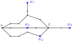
While storing additional information per label increases the space consumption, it is important to note that we do not need to store global edge IDs here, but it suffices to have local ID for the edges incident to w. Therefore, with ∆(w) denoting the degree of w, we only need log∆(w) additional bits.
5 Bounded Suboptimal PC-LHL
For many applications, finding a path from s to t that has close to optimal cost is sufficient [Shen et al., 2022]. The goal of a bounded suboptimal pathfinding algorithm is to efficiently identify a path π′ with c(π′ ) < α · c(π) where π is the optimal path and α is the chosen approximation factor.
A simple way to reduce query time of LHL when performing bounded suboptimal pathfinding is to check whether UB ≤ α · LB. In this case, reporting the path that corresponds to the UB is sufficient. If one is only interested in a distance estimate within a factor α of the correct value, it even suffices to have UB ≤ 2α ·LB and then to report the average of UB and LB similar to the approach proposed in [Potamias et al., 2009]. While this accelerates query answering, it does not tap into the potential of constructing a smaller labeling that adheres to α in the first place. Next, we will investigate methods to obtain such labelings. We start by describing a labeling method that ensures a bounded additive detour, that is, c(π′ ) ≤ c(π) + β. We call such a labeling a β-labeling. Subsequently, we discuss how to use a given β-labeling to answer LHL queries with an α-approximate guarantee.
5.1 Center Hub Labeling
The basic idea of constructing a concise labeling with additive detour bound β is to only allow a (small) subset of nodes to become hubs. These hubs should be nicely spread over the graph. To achieve this, we map our hub selection problem to that of identifying centers in a graph. The famous k-center problem asks for a given graph G(V,E) to select a subset C ⊂ V, |C| = k of center nodes, such that the largest shortest path distance of any node to its nearest center is minimized. The problem is NP-hard but a simple greedy algorithm yields a 2-approximation [Gonzalez, 1985]. The algorithm starts by selecting an arbitrary node in the first round. Then, in the following k - 1 rounds, it always selects the node with largest distance to all previously selected ones. Accordingly, the objective function value decreases monotonically over the course of the algorithm. We use this algorithm for selecting a set of center-hubs C by not fixing k a priori but proceeding to select new nodes until the shortest path distance of any node to its nearest center falls below the threshold of β/2.
Given a valid HHL and a set of center hubs C, we proceed as follows to obtain a β-labeling: We first run Dijkstra's algorithm on all nodes in C at once. The resulting forest consists exactly of |C| shortest path trees where each tree contains the nodes that have the tree root as their closest center. We store this center information C(w) with each node w ∈ V . Furthermore, we compute the full shortest path trees from each node in C individually. Then, for every v ∈ V , we modify its labeling by replacing w ∈ L(v) with C(w) and also updating the corresponding distance value based on the precomputed shortest path trees. The hope, of course, is that many w ∈ L(V ) are mapped to the same center hub and thus the label size decreases. After the label modifications are done, all other precomputed information can be deleted. The resulting labeling is a valid β-labeling, as for any two nodes s, t with a perfect hub h there is now C(h) in L(s)∩L(t) and the detour from h to C(h) is at most 2 · β/2 = β.
5.2 Bounded Suboptimal LHLQueries
For PC-LHL, we proceed as described above for HHL and replace all label nodes with their closest centers and also update the distances accordingly. During query answering, we first perform the PC-LHL query algorithm as before, getting a lower and an upper bound. As both these bounds are still valid with respect to c(π), upper bound path reporting can be used if the two bounds are within a factor of α. If that is not the case, the lower bound needs to be checked. Here, we run into the problem that a node w that was a perfect landmark for s, t before might now have been replaced with a node C(w) such that w.l.o.g t is no longer on the shortest path from s to C(w). To compensate for that, we run A* from s, using the distances to the center nodes as landmark information. More precisely, we determine the set of center nodes in L(s)∩L(t) that imply a lower bound smaller than UB. Then, in the A* search, we only consider those center nodes as landmarks. Nodes that do not have any of these center nodes in their label can be immediately excluded from the search. Once t is found, we have the exact shortest path. The search can also be aborted if the search radius exceeded the weakest lower bound that is under inspection or if the best distance estimate to the target exceeds UB/α. In these cases, upper bound (reporting) provides a query result within the specified α-bound.
Note that while β needs to be known to the preprocessing algorithm, α can be chosen on query time.
6 Experimental Study
We implemented all described algorithms in C++. As benchmarks, we used grid and road networks of different size. For grid networks, we used the Baldurs Gate II game maps from an established 2D pathfinding benchmark [Sturtevant, 2012]. This set contains 120 octile maps in their original size (BGIIori) and 75 maps scaled to a 512x512 grid (BGII512). The maps contain up to 231,469 accessible grid cells. To have road networks of different sizes, we ran Dijkstra's algorithm from randomly selected nodes in the European road network (extracted from OpenStreetMap 1 ) until n nodes were settled, and used their induced subgraphs. Experiments were conducted on a single core of an AMD Ryzen 7 PRO 6850U Processor clocked at 3,2GHz and using up to 32 GB RAM.
| ALT-10 | ALT-25 | ALT-50 | ||||
|---|---|---|---|---|---|---|
| CH | KC | CH | KC | CH | KC | |
| ROAD1M | 0.30 | 0.11 | 0.24 | 0.05 | 0.16 | 0.03 |
| BGII512 | 0.37 | 0.12 | 0.16 | 0.09 | 0.15 | 0.08 |
6.1 Node Ranking and Landmark Selection
All preprocessing algorithms for HPC-LHL computation presented in this paper rely on a node ranking r. For MaxHit, the ranking results from the order in which the greedy hitting set algorithm selects the nodes. For TreeSelect and HHL pruning, r can be chosen freely. As discussed above, HHL can be computed on the basis of a CH and by this inherits its ranking function. We use the CH implementation described by [Geisberger et al., 2012] and refer to the resulting r as CHorder. HHL with CH-order is the baseline we use to compare the label sizes of our HPC-LHL against. We could also use CH-order for HPC-LHL. However, in a CH-order nodes with a high rank are typically in the middle part of many long shortest paths. This is ideal for CH and also for HHL. But HPC-LHL integrates landmark-based bounds in the labeling. These bounds are the weakest if the node is in the middle of the shortest path between source and target (as then their absolute path difference towards the landmark is close to zero). To also have strong landmarks with high ranks, we proceed as follows: We first compute a greedy k-center order as described for bounded suboptimal pathfinding. Then, we take the first 5% of the nodes in this order and assign them the highest ranks. For the remaining nodes, we proceed with the CH-order. The resulting order is used below for TreeSelect as well as the HHL pruning algorithms.
To illustrate that the k-center ranking, referred to as KCorder from now on, indeed produces good landmarks, we conducted the following experiment: We implemented the classical ALT algorithm [Goldberg and Harrelson, 2005] and let the landmarks be the nodes of highest rank either in the CHorder or in the KC-order. For both variants, we measured the fraction of nodes visited in the A* search and in the Dijkstra search. Table 1 shows the average results over 100 random queries per instance in BGII512 and 100 road networks with n = 106 , using 10, 25 or 50 landmarks. We see a significant reduction across all instances when using the KC-order over the CH-order. Indeed, 50 landmarks chosen in CH-order are not even as powerful as 10 landmarks chosen in KC-order. Although a larger number of landmarks leads to an even more pronounced reduction in the size of the search space, it also takes longer to compute the distance estimate. Using 25 landmarks resulted in the best query times on average. Thus, we use ALT with the top 25 nodes according to the KC-order as the baseline for query answering below.
1 https://i11www.iti.kit.edu/resources/roadgraphs.php
6.2 Preprocessing Algorithms
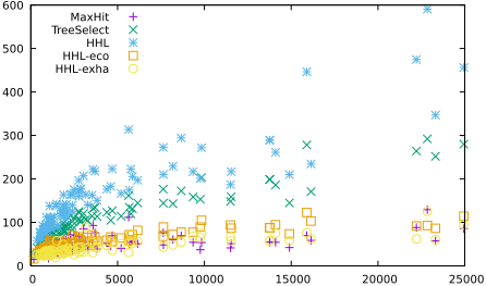
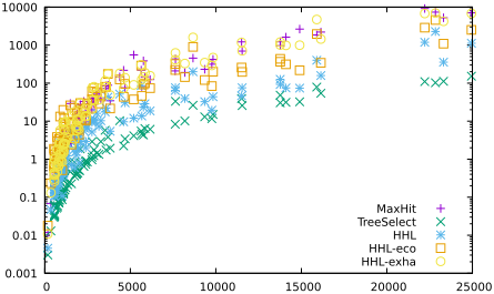
Next, we strive to compare the different preprocessing algorithms for exact HPC-LHL discussed in the paper: MaxHit, TreeSelect, HHL, exhaustive HHL pruning (HHL-exha) as well as economic HHL pruning (HHL-eco). To have comparative results for all methods, we first consider the 116 maps in BGIIori with up to 25,000 nodes. Figure 2 shows the average label sizes and Figure 3 depicts the running times for each instance. Table 2 shows the running times and the average and maximum label sizes averaged over all instances. Our main observations are as follows: HHL-exha performs best with respect to average and maximum label size. While it is a bit slower than MaxHit, it only needs a fraction of its space. Indeed, for inputs with about 10,000 nodes, the number of maximal shortest paths was already well above 10 million. For the map AR001 with 22,216 nodes it was close to 116 million paths. For maps with more than 25,000 nodes, MaxHit exceeded our storage capabilities. TreeSelect is very fast on small graphs but does produce label sizes more than twice als large as those of MaxHit and HHL-exha. The canonical HHL is also fast to compute but we see that both pruning approaches, HHL-eco and HHL-exha, lead to a remarkable reduction in label size. This already illustrates that the flexibility of LHL to ensure tight distance bounds via hubs or landmarks is clearly beneficial on grid networks.
| time | Lavg | Lmax | |
|---|---|---|---|
| MaxHit | 400.2 | 44.4 | 87.3 |
| TreeSelect | 8.9 | 99.5 | 218.9 |
| HHL | 60.6 | 149.4 | 312.7 |
| HHL-eco | 166.2 | 53.6 8 | 118.4 |
| HHL-exha | 376.6 | 39.3 | 77.9 |
For the large grid instances (BGII512), we restricted our tests to TreeSelect, HHL and HHL-eco. The trends observed for the smaller data sets continued here. TreeSelect remained about on order of magnitude faster than HHL, with an average running time of 8 to 10 minutes, while the running time for HHL computation was about 1 to 2 hours, depending on the structure of the network. HHL-eco took another 4 to 8 hours per instance. This complies well with our theoretical analysis of HHL and HHL-eco, where HHL takes time proportional to nL2max and HHL-eco proportional to mL2avg and m being roughly a factor of 4 larger than n in octile grids. But the investment of preprocessing time is worthwhile, as the number of labels was reduced on average by more than 50% with HHL-eco compared to TreeSelect and by more than 70% compared to HHL, for both average and max label size.
For road networks, we obtained results that deviated from those for grid maps: For a comparable number of nodes, HHL sizes were significantly lower for road networks. For example, for road networks with around 100,000 nodes the average HHL label size was only about 50 to 60 while the average for grids was 500 to 1000. As a result, canonical HHL computation was much faster on road networks and even outperformed TreeSelect. For 100,000 nodes, HHL only took about 30 seconds while the running time of TreeSelect approached half an hour. HHL-exha produced labels that are up to 50% smaller than the ones in the HHL. But the running time was already over 3 hours for 100,000 nodes and thus we did not apply it to even larger road networks. HHL-eco was almost as fast as HHL computation itself, which complies with our running time analysis and the average node degree of slightly above 2 in typical road networks. However, HHL-eco only provided a reduction in average label size of about 5-10%, which is a significantly smaller reduction margin than the one achieved on grids. But the maximum label size was reduced by up to 27%. For graphs with 1 million nodes, we got for HHL Lavg = 133.4 and Lmax = 286.2 in roughly 45 minutes. After applying HHL-eco, which took another hour, we got Lavg = 123.8 and Lmax = 198.8. Despite the reduction in label size being not as pronounced as for grids, every subtraction from Lavg implies a space reduction proportional to n. Furthermore, a reduced maximum label size is beneficial for query answering as we will discuss in more detail below.
6.3 Query Answering
For HPC-LHL query answering, we measured how often only the upper bound UB was tight, how often only the lower bound LB was tight, and how often they were equal. Furthermore, in case LB < UB, we counted how often the proposed edge oracle led to conclusive results without the need of a lower bound path check. On average over 1000 queries per large instance, using HHL-eco, we got 77.6% queries where the UB is tight, 53.3% queries in which the LB was tight, 30.9% in which both are tight and 69,1% in which an LB check was needed. The edge oracle was conclusive in 23% of the cases in question. The speed-up over ALT for both distance and path queries was over 50,000 for HPC-LHL. For path queries, HPC-LHL was even faster than HHL, as the smaller label sizes outweighed the path check time. For distance queries, HHL was about 1.4 times faster than HPC-LHL but here the running time was anyway in the order of 1-2 microseconds. We conclude that HPC-LHL maintains the high speed-up of labeling techniques while reducing the label size.
6.4 Bounded Suboptimal LHL
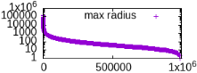
Finally, we examine how the label sizes and the query times are affected if the query algorithm is allowed to return a path that is at most α times longer than the optimal path. Figure 4 shows the maximum distance (also called β-radius) of any node to its nearest selected center after each round of selection. We see a steep decay in this radius which implies that restricting the labels to a small subset of the nodes suffices to get a valid β-labeling for given β. Using β =5 kilometers in road networks with n = 106 nodes yielded a center set of size 1,494 and reduced the average label size from 131.7 to 81.5. Choosing α = 1.05, in over 98% of random queries, upper bound path reporting was valid. In the remaining cases, the refined ALT search space was only about 3 to 5 times the number of nodes on the shortest path. Other trade-offs can easily be achieved by adjusting α and β. For grids, we used hop-bounds for β and also observed great flexibility in trading path quality against label size and query time.
7 Conclusions and FutureWork
We showed that LHL is a very effective labeling technique, which produces significantly smaller label sizes than previous approaches (especially on grid networks) while also achieving very fast query times. One possible direction for future work is the careful parallelization of the pruning algorithms to make them applicable to even larger inputs. With methods like PHAST [Delling et al., 2013a], which is CH-based, all pair shortest paths can be computed in reasonable time even for large road networks. Adapting this method to accelerate pruning seems to be promising. Furthermore, there might be ranking functions that lead to even smaller labelings than the ones produced by our combination of center-order and CHorder. Incorporating other known methods that select good landmarks for A* could result in further improvements.
@inproceedings{ijcai2024p750,
  title     = {Scalable Landmark Hub Labeling for Optimal and Bounded Suboptimal Pathfinding},
  author    = {Storandt, Sabine},
  booktitle = {Proceedings of the Thirty-Third International Joint Conference on
               Artificial Intelligence, {IJCAI-24}},
  publisher = {International Joint Conferences on Artificial Intelligence Organization},
  editor    = {Kate Larson},
  pages     = {6788--6795},
  year      = {2024},
  month     = {8},
  note      = {Main Track},
  doi       = {10.24963/ijcai.2024/750},
  url       = {https://doi.org/10.24963/ijcai.2024/750},
}
TY - CPAPER TI - Scalable Landmark Hub Labeling for Optimal and Bounded Suboptimal Pathfinding AU - Storandt, Sabine T2 - Proceedings of the Thirty-Third International Joint Conference on Artificial Intelligence, IJCAI-24 PB - International Joint Conferences on Artificial Intelligence Organization PY - 2024 SP - 6788 EP - 6795 DO - 10.24963/ijcai.2024/750 UR - https://doi.org/10.24963/ijcai.2024/750 ER -Copied
Machine-readable versions of this paper, for tools and AI agents:





