
A Better Approximation for Bipartite Traveling Tournament in Inter-League Sports Scheduling
Proceedings of the Thirty-Third International Joint Conference on Artificial Intelligence. Main Track. Pages 6814-6822.
https://doi.org/10.24963/ijcai.2024/753
Keywords
- Planning and Scheduling: PS: Scheduling
- Planning and Scheduling: PS: Theoretical foundations of planning
- Planning and Scheduling: PS: Routing
Abstract
The bipartite traveling tournament problem (BTTP) was initially introduced by Hoshino and Kawarabayashi (AAAI 2011) to address inter-league sports scheduling, which aims to design a feasible bipartite tournament between two n-team leagues under some constraints such that the total traveling distance of all participating teams is minimized. Since its introduction, several heuristic methods have been developed to design feasible schedules for NBA, NPB and so on. In terms of solution quality with a theoretical guarantee, previously only a (2+ε) approximation is known for the case that n≡0 (mod 3). Whether there are similar results for the cases that n≡1 (mod 3) and n≡2 (mod 3) was asked in the literature. In this paper, we answer this question positively by proposing a (3/2+ε)-approximation algorithm for any n and any constant ε>0, which also improves the previous ratio for the case that n≡0 (mod 3).
- [Anagnostopoulos et al., 2006] Aris Anagnostopoulos, Lau- rent Michel, Pascal Van Hentenryck, and Yannis Verga- dos. A simulated annealing approach to the traveling tour- nament problem. Journal of Scheduling, 9(2):177-193, 2006.
- [Bulck et al., 2020] David Van Bulck, Dries R. Goossens, Jörn Schönberger, and Mario Guajardo. Robinx: A three- field classification and unified data format for round-robin sports timetabling. European Journal of Operational Re- search, 280(2):568-580, 2020.
- [Chatterjee and Roy, 2021] Diptendu Chatterjee and Bi- mal Kumar Roy. An improved scheduling algorithm for traveling tournament problem with maximum trip length two. In ATMOS 2021, volume 96, pages 16:1-16:15, 2021.
- [Di Gaspero and Schaerf, 2007] Luca Di Gaspero and An- drea Schaerf. A composite-neighborhood tabu search ap- proach to the traveling tournament problem. Journal of Heuristics, 13(2):189-207, 2007.
- [Durán, 2021] Guillermo Durán. Sports scheduling and other topics in sports analytics: a survey with special ref- erence to latin america. Top, 29(1):125-155, 2021.
- [Easton et al., 2001] Kelly Easton, George Nemhauser, and Michael Trick. The traveling tournament problem: de- scription and benchmarks. In CP 2001, pages 580-584, 2001.
- [Easton et al., 2002] Kelly Easton, George L. Nemhauser, and Michael A. Trick. Solving the travelling tournament problem: A combined integer programming and constraint programming approach. In PATAT 2002, volume 2740 of Lecture Notes in Computer Science, pages 100-109. Springer, 2002.
- [Frohner et al., 2023] Nikolaus Frohner, Bernhard Neu- mann, Giulio Pace, and Günther R Raidl. Approaching the traveling tournament problem with randomized beam search. Evolutionary Computation, 31(3):233-257, 2023.
- [Goerigk and Westphal, 2016] Marc Goerigk and Stephan Westphal. A combined local search and integer program- ming approach to the traveling tournament problem. An- nals of Operations Research, 239(1):343-354, 2016.
- [Goerigk et al., 2014] Marc Goerigk, Richard Hoshino, Ken-ichi Kawarabayashi, and Stephan Westphal. Solving the traveling tournament problem by packing three-vertex paths. In AAAI 2014, pages 2271-2277. AAAI Press, 2014.
- [Hartvigsen, 1984] David Hartvigsen. Extensions of match- ing theory. PhD thesis, Carnegie-Mellon University, 1984.
- [Hentenryck and Vergados, 2007] Pascal Van Hentenryck and Yannis Vergados. Population-based simulated anneal- ing for traveling tournaments. In AAAI 2007, pages 267- 272. AAAI Press, 2007.
- [Hoshino and Kawarabayashi, 2011a] Richard Hoshino and Ken-ichi Kawarabayashi. The distance-optimal inter- league schedule for japanese pro baseball. In Proceed- ings of the ICAPS 2011 Workshop on Constraint Satis- faction Techniques for Planning and Scheduling Problems (COPLAS), pages 71-78, 2011.
- [Hoshino and Kawarabayashi, 2011b] Richard Hoshino and Ken-ichi Kawarabayashi. The inter-league extension of the traveling tournament problem and its application to sports scheduling. In AAAI 2011, pages 977-984, 2011.
- [Hoshino and Kawarabayashi, 2011c] Richard Hoshino and Ken-ichi Kawarabayashi. Scheduling bipartite tourna- ments to minimize total travel distance. Journal of Arti- ficial Intelligence Research, 42:91-124, 2011.
- [Hoshino and Kawarabayashi, 2012] Richard Hoshino and Ken-ichi Kawarabayashi. The linear distance traveling tournament problem. In AAAI 2012, pages 1770-1778. AAAI Press, 2012.
- [Hoshino and Kawarabayashi, 2013] Richard Hoshino and Ken-ichi Kawarabayashi. An approximation algorithm for the bipartite traveling tournament problem. Mathematics of Operations Research, 38(4):720-728, 2013.
- [Imahori, 2021] Shinji Imahori. A 1+O(1/N) approximation algorithm for TTP(2). CoRR, abs/2108.08444, 2021.
- [Kendall et al., 2010] Graham Kendall, Sigrid Knust, Celso C Ribeiro, and Sebastián Urrutia. Scheduling in sports: An annotated bibliography. Computers & Operations Research, 37(1):1-19, 2010.
- [Lim et al., 2006] Andrew Lim, Brian Rodrigues, and Xing- wen Zhang. A simulated annealing and hill-climbing algorithm for the traveling tournament problem. Eu- ropean Journal of Operational Research, 174(3):1459- 1478, 2006.
- [Miyashiro et al., 2012] Ryuhei Miyashiro, Tomomi Matsui, and Shinji Imahori. An approximation algorithm for the traveling tournament problem. Annals of Operations Re- search, 194(1):317-324, 2012.
- [Thielen and Westphal, 2011] Clemens Thielen and Stephan Westphal. Complexity of the traveling tournament prob- lem. Theoretical Computer Science, 412(4):345-351, 2011.
- [Thielen and Westphal, 2012] Clemens Thielen and Stephan Westphal. Approximation algorithms for TTP(2). Math- ematical Methods of Operations Research, 76(1):1-20, 2012.
- [Trick, 2024] Michael Trick. Challenge traveling tournament instances. Online, 2024.
- [Westphal and Noparlik, 2014] Stephan Westphal and Karl Noparlik. A 5.875-approximation for the traveling tournament problem. Annals of Operations Research, 218(1):347-360, 2014.
- [Williamson and Shmoys, 2011] David P Williamson and David B Shmoys. The design of approximation algo- rithms. Cambridge university press, 2011.
- [Xiao and Kou, 2016] Mingyu Xiao and Shaowei Kou. An improved approximation algorithm for the traveling tour- nament problem with maximum trip length two. In MFCS 2016, volume 58 of LIPIcs, pages 89:1-89:14, 2016.
- [Yamaguchi et al., 2011] Daisuke Yamaguchi, Shinji Ima- hori, Ryuhei Miyashiro, and Tomomi Matsui. An im- proved approximation algorithm for the traveling tourna- ment problem. Algorithmica, 61(4):1077-1091, 2011.
- [Zhao and Xiao, 2021a] Jingyang Zhao and Mingyu Xiao. A further improvement on approximating TTP-2. In CO- COON 2021, volume 13025 of Lecture Notes in Computer Science, pages 137-149, 2021.
- [Zhao and Xiao, 2021b] Jingyang Zhao and Mingyu Xiao. The traveling tournament problem with maximum tour length two: A practical algorithm with an improved ap- proximation bound. In IJCAI 2021, pages 4206-4212, 2021. IJCAI
- [Zhao and Xiao, 2023] Jingyang Zhao and Mingyu Xiao. The linear distance traveling tournament problem allows an EPTAS. In AAAI 2023, pages 12155-12162, 2023.
- [Zhao et al., 2022] Jingyang Zhao, Mingyu Xiao, and Chao Xu. Improved approximation algorithms for the travel- ing tournament problem. In MFCS 2022, volume 241 of LIPIcs, pages 83:1-83:15, 2022.
References were extracted automatically from the PDF and may contain errors.
Full text extracted automatically from the PDF; figures, tables and equations may differ. The PDF is the version of record.
1 Introduction
The traveling tournament problem (TTP), introduced by Easton et al. [2001], is a well-known benchmark problem in the field of sports scheduling [Kendall et al., 2010]. This problem aims to find a double round-robin tournament, minimizing the total traveling distance of all participating teams. In a double round-robin tournament involving n teams (where n is even), each team plays two games against each of the other n - 1 teams that includes one home game at its own home venue and one away game at its opponent's home venue, and on each day each team can only play one game. Moreover, all games should be scheduled on 2(n-1) consecutive days, subject to several constraints on the maximum number of consecutive home/away games for each team, ensuring a balanced tournament arrangement. In the problem, we may also consider that the distance is a semi-metric, i.e., it satisfies the symmetry and triangle inequality properties. An overview of TTP and its variants, along with their various applications on sports scheduling, can be found in [Bulck et al., 2020; Dur´an, 2021].
∗Contact Author
The bipartite traveling tournament problem (BTTP), introduced by Hoshino and Kawarabayashi [2011b], is an interleague extension of TTP. Given two n-team leagues, it asks for a distance-optimal double round-robin bipartite tournament between the leagues, where every team in one league plays one home game and one away game against each team in another league. It also requires that each team plays only one game on each day, and all games need to be scheduled on 2n consecutive days. For TTP/BTTP, the double round-robin (bipartite) tournament is subject to the following three basic constraints or assumptions:
- No-repeat: No pair of teams can play against each other in two consecutive games.
- direct-traveling: Each team travels directly from its game venue on the i-th day to its game venue on the (i + 1)-th day, where we assume that all teams are initially at home before the first game starts and will return home after the last game ends.
- Bounded-by-3: Each team can play at most 3consecutive home games or away games.
In the last constraint, we require that the maximum number of consecutive home/away games for each team is at most three. This is the most extensively studied case [Lim et al., 2006; Anagnostopoulos et al., 2006; Goerigk et al., 2014]. The case that at most two consecutive home/away games are allowed is also studied in some references [Thielen and Westphal, 2012; Chatterjee and Roy, 2021; Zhao and Xiao, 2021b]. A small number of consecutive home/away games requires teams to return home frequently, which may make the tournament balanced as a cost of a possible longer traveling distance.
As indicated in a previous study [Hoshino and Kawarabayashi, 2011c], BTTP has natural applications in sports scheduling, such as for events like the Davis Cup, the biennial Ryder Cup, the National Basketball Association (NBA), and the Nippon Professional Baseball (NPB). Exploring BTTP also holds promise for advancing the theoretical development of enhanced algorithms for TTP. For instance, Zhao and Xiao [2023] utilized an approximation algorithm for BTTP between two groups by grouping teams and achieved an efficient polynomial-time approximation scheme for a special case of TTP where all teams are positioned along a line. BTTP possesses a simpler structure, and scheduling for TTP can be derived from scheduling for BTTP using a divide-and-conquer method [Chatterjee and Roy, 2021]. Therefore, effective algorithms for BTTP have the potential to yield effective algorithms for TTP as well.
1.1 RelatedWork
Both TTP and BTTP are difficult optimization problems, and their NP-hardness has been established in [Thielen and Westphal, 2011; Hoshino and Kawarabayashi, 2011b]. In the online benchmark [Trick, 2024; Bulck et al., 2020], many instances of TTP with more than ten teams have not been completely solved even by using high-performance machines. TTP and BTTP have been extensively studied both in theory [Hoshino and Kawarabayashi, 2012; Hoshino and Kawarabayashi, 2013; Westphal and Noparlik, 2014; Xiao and Kou, 2016; Imahori, 2021; Zhao and Xiao, 2021a] and practice [Easton et al., 2002; Di Gaspero and Schaerf, 2007; Hentenryck and Vergados, 2007; Hoshino and Kawarabayashi, 2011a; Hoshino and Kawarabayashi, 2011b; Hoshino and Kawarabayashi, 2011c; Goerigk and Westphal, 2016; Frohner et al., 2023].
TTP and BTTP are also rich problems in approximation algorithms. An algorithm is called an α-approximation algorithm if it can generate a feasible schedule in polynomial time such that the total traveling distance of all teams is within α times the optimal. For TTP, Miyashiro et al. [2012] first proposed a (2 + ε)-approximation algorithm where ε is an arbitrary fixed constant, and the ratio was later improved to (1.667 + ε) by Yamaguchi et al. [2011], and (1.598 + ε) by Zhao et al. [2022]. For BTTP, the only known result is a (2 + ε)-approximation algorithm for the case that n ≡ 0 (mod 3), proposed by Hoshino and Kawarabayashi [2013], and whether there exist similar algorithms for the cases that n ≡ 1 (mod 3) and n ≡ 2 (mod 3) was asked in this paper.
1.2 Our Results
In this paper, we design a new algorithm for BTTP and prove that our algorithm can achieve an approximation ratio of (3/2 + ε) for any n and any constant ε > 0. This not only positively answers the open question for the cases that n ≡ 1 (mod 3) and n ≡ 2 (mod 3) but also improves the previous best ratio of (2+ε) for the case that n ≡ 0 (mod 3) [Hoshino and Kawarabayashi, 2013].
To achieve our improvement, we introduce a novel lower bound for BTTP related to the minimum weight cycle packing (i.e., a set of cycles and each cycle has a length of at least 3). Then, we propose a 3-path packing construction, which reduces BTTP to the task of finding a good 3-path packing. At last, we use the minimum weight cycle packing to obtain a 3-path packing, and show that by applying the 3-path packing to our construction we can get a schedule with an approximation ratio of at most (3/2 + ε) in polynomial time.
In addition to the theoretical results, we also consider the practical applications of our construction. We create a new instance from the real situation of NBA for BTTP with 32 teams (n = 16) and test our algorithm on this instance. Note that previous construction only works for the case that n ≡ 0 (mod 3). In the new instance, n ≡ 1 (mod 3). We extend our 3-path packing construction to a more efficient construction based on 3-cycles. By applying these two constructions to the new instance, experimental results show that our algorithms can be implemented within 2 seconds, and the quality of the obtained solutions is much better than the expected 1.5-approximation ratio: the gaps between our results and the optimal are at most 24.66% and 9.42% for the 3-path and 3cycle constructions.
Due to limited space, the proofs of lemmas and theorems marked with "*" were omitted and they can be found in the full version of this paper.
2 Notations
An instance of BTTP can be presented by a complete graph G = (V = X ∪ Y, E, w) with 2n vertices representing 2n teams, where X = {x0, . . . , xn-1} and Y = {y0, . . . , yn-1} are two n-team leagues, and w is a non-negative semi-metric weight function on the edges in E that satisfies the symmetry and triangle inequality properties, i.e., w(x, y) + w(y, z) ≥ w(x, z) = w(z, x) for any x, y, z ∈ V . The weight w(x, y) of edge xy ∈ E represents the distance between the homes of teams x and y. We also extend the function to a set of edges, i.e., we let w(E′ ) := ∑e∈E′ w(e) for any E′ ⊆ E, and to a subgraph G′ of G, i.e., we let w(G′ ) be the total weight of all edges in G′ . Given any V ′ ⊆ V , the complete graph induced by V ′ is denoted by G[V ′ ].
Given two vertices/teams x ∈ X and y ∈ Y , and two sets X′ ⊆ X and Y ′ ⊆ Y , we define the following notations. We use x → y to denote a game between x and y at the home of y, and x ↔ y to denote two games between x and y including one game at the home of x and one game at the home of y. We use EY ′(x) (resp., EX′(y)) to denote the set of edges in G between the vertex x (resp., y) and one vertex in Y ′ (resp., X′ ), i.e., EY ′(x) = {xy | y ∈ Y ′ }. We also let δY ′ (x) = w(EY ′ (x)) and δY ′ (X′ ) = ∑x∈X′ δY ′ (x) (resp., δX′ (y) = w(EX′ (y)) and δX′ (Y ′ ) = ∑y∈Y ′ δX′ (y)). Note that δY ′ (X′ ) = δX′ (Y ′ ).
Two subgraphs or sets of edges are vertex-disjoint if they do not share a common vertex. An l-cycle x1x2 . . . xlx1 is a simple cycle on l different vertices {x1, . . . , xl}. It consists of l edges {x1x2, . . . , xlx1}, and its length is said to be l. A cycle packing in a graph is a set of vertex-disjoint cycles, where the length of each cycle is at least three and the cycles cover all vertices of the graph. The minimum weight cycle packing in a graph with n vertices can be found in O(n3 ) time [Hartvigsen, 1984]. Similarly, an l-path x1x2 . . . xl is a simple path on l different vertices {x1, . . . , xl}. It consists of l - 1 edges {x1x2, . . . , xl-1xl}, and the vertices x1 and xl are called its terminals. An l-path packing in a graph is a set of vertex-disjoint l-paths, where the paths cover all vertices of the graph.
A walk is a sequence of vertices where each consecutive pair of vertices is connected by an edge, and its weight is defined as the total weight of the edges traversed in the sequence. A walk is closed if the first and the last vertices are the same. In a solution of BTTP, every team v ∈ X ∪ Y has an itinerary, which is a closed walk starting and ending at v. This itinerary could be decomposed into several minimal closed walks, each starting and ending at v, referred to as trips. Each trip is an l-cycle containing v with 2 ≤ l ≤ 4, and all trips/cycles share only one common vertex v. For example, Table 1 shows a solution for leagues X = {x0, x1, x2} and Y = {y0, y1, y2}, where home games are marked in bold. We can get that x2 has an itinerary x2y0y1y2x2, and y2 has an itinerary y2x1x2y2x0y2, and y2 has two trips y2x1x2y2 and y2x0y2 (a 3-cycle and a 2-cycle sharing y2 only).
| 0 | 1 | 2 | 3 | 4 | 5 | |
|---|---|---|---|---|---|---|
| x0 | y0 | y1 | y2 | y0 y0 y0 | y1 y1 y1 | y2 y2 y2 |
| x1 | y2 y2 y2 | y0 | y1 | y2 | y0 y0 y0 | y1 y1 y1 |
| x2 | y1 y1 y1 | y2 y2 y2 | y0 | y1 | y2 | y0 y0 y0 |
| y0 | x0 x0 x0 | x1 x1 x1 | x2 x2 x2 | x0 | x1 | x2 |
| y1 | x2 | x0 x0 x0 | x1 x1 x1 | x2 x2 x2 | x0 | x1 |
| y2 | x1 | x2 | x0 x0 x0 | x1 x1 x1 | x2 x2 x2 | x0 |
Fix a constant ε > 0. We want to consider a 3-path packing in G. Since n may not be divisible by 3, we will remove a small number of vertices (as we will see that the number is related to ε) in X and Y to obtain two new sets Xε ⊆ X and Yε ⊆ Y such that the number of vertices in Xε and Yε, denoted as nε, are the same and can be divisible by 3. Hence, there always exist 3-path packings in G[Xε] and G[Yε]. We also let Xε := X \ Xε and Yε := Y \ Yε. The graph Gε := G[Xε ∪ Yε] is called the core graph of G because we will see that the quality of our schedule is only dominated by the total traveling distance of teams in Xε ∪Yε, i.e., the total traveling distance of teams in Xε∪Yε is small. We denote the minimum weight cycle packing in G[Xε] (resp., G[Yε]) by CXε (resp., CYε ).
3 Lower Bounds
Lower bounds play an important role in approximation algorithms. We need to compare our solution with the optimal solution. However, it is hard to compute the optimal solution. Then, we turn to find some lower bounds of the optimal value and compare our solution with the lower bounds. We will use two lower bounds. The first one is from the literature and the second one is newly proved. We use OPT to denote the weight (i.e., the total traveling distance of all teams) of an optimal solution for BTTP.
Next, we will propose a new lower bound that is related to the minimum weight cycle packings CXε and CYε .
4 The Construction of the Schedule
Assuming we are given a 3-path packing PXε in G[Xε] and a 3-path packing PYε in G[Yε], to construct a schedule that minimizes the total traveling distance of teams inXε∪Yε, the idea is to ensure every team in Xε (res., Yε) plays 3-consecutive away games along every 3-path in PYε (resp., PXε ) from one terminal to another.
Consider an ideal schedule where every team in Yε (resp., Xε) plays 3-consecutive away games along every 3-path in PXε (resp., PYε ). Then, every team in Yε (resp., Xε) plays nε 3 away-trips with teams in Xε (resp., Yε). The total traveling distance of teams in Yε for these away-trips is
Denote ∑xx′ x′′∈PXε (δYε (x)+δYε (x′′ )) by δYε (PXε ) for the sake of presentation and define δXε (PYε ) in the similar manner. The total traveling distance of teams in Xε ∪Yε for these away-trips is δYε (PXε )+nεw(PXε )+δXε (PYε )+nεw(PYε ).
Our construction will generate a schedule such that the total traveling distance of teams inX∪Y is close to δYε (PXε )+ nεw(PXε ) + δXε (PYε ) +nεw(PYε ), i.e, the performance of our schedule is close to the ideal schedule. To achieve this, we make sure that almost every team in Yε (resp., Xε) plays 3-consecutive away games along every 3-path in PXε (resp., PYε ). Next, we give our construction in details.
Note that ε > 0 is a fixed constant. Let d := 6⌈1/ε⌉ and m := 2⌊ n 6d ⌋ - 1 (it is useful to ensure that d is even and m is odd). We will select nε := 3md vertices from X (resp., Y ) to formXε (resp., Yε). The details of how to select these vertices is deferred to the analysis part of our schedule. Recall that PXε and PYε are two given 3-path packings in G[Xε] and G[Yε]. So, both PXε and PYε contain md 3-paths. Assume that PXε = {P1, . . . , Pmd} and PYε = {Q1, . . . ,Qmd}, where Pi = x3i-3x3i-2x3i-1 and Qi = y3i-3y3i-2y3i-1. Each 3-path corresponds to three teams. For every d 3-paths from P1 (resp., Q1) to Pmd (resp., Qmd), we pack the corresponding 3d teams as a super-team, denoted by Si (resp., Ti). So, Si = {x3i′-3, x3i′-2, x3i′-1}id-1 i′=id-d . Let l := n - nε. There are l teams in Xε (resp., Yε), and we label them using {xnε , . . . , xn-1} (resp., {ynε , . . . , yn-1}). We can get l team-pairs {L1, . . . , Ll} where Li = {xnε+i-1, ynε+i-1}.
We may assume that n ≥ 108d3 , as otherwise, we have n < 108d3 = Oε(1)1 , and in this case, we can solve the problem optimally in constant time. Since n ≥ 108d3 , we can get m ≥ 18d2 . Moreover, since l = n-nε = n-3md = n - 6d⌊ n 6d ⌋ + 3d, we can get 3d ≤ l ≤ 9d ≤ m.
The main idea of the construction is that: we first arrange a schedule of super-games between super-teams (including the team-pairs); then, we extend the super-games into normal games between normal teams, which will form a feasible schedule for BTTP.
Our schedule contains m + 1 time slots, where we have m super-games in each of the first m time slots, including l left super-games and m-l normal super-games. Each superteam will attend one super-game in each of the first m time slots. The last time slot is special, and we will explain it later. Each of the first m time slots spans 6d days and the last time slot spans 2l days. Hence, our schedule will span 6md + 2l = 2nε + 2l = 2n days.
1Oε(1) means a constant related to ε.
4.1 The First mTime Slots
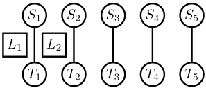
In the first time slot, the super-games are arranged as shown in Figure 1, where m = 5 and l = 2. Each super-team is denoted by a cycle node and each team-pair is denoted by a square node. There are 2m super-teams, l team-pairs, and m super-games. Each super-game is denoted by an edge between two super-teams. The most left l super-games, each involving two super-teams and one team-pair, are called the left super-games. The left super-game involving team-pair Li is denoted as the i-th left super-game. The other m- l super-games are called normal super-games. It is worth noting that there are only a constant number of left super-games since l ≤ 9d = Oε(1). So, in our construction almost all super-games are normal super-games.
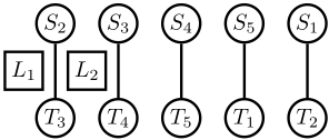
In the second time slot, the super-games are arranged as shown in Figure 2. Compared to the first time slot, the positions take one leftward shift for super-teams S1, . . . , Sm, take two leftward shifts for super-teams T1, . . . , Tm, and keep unchanged for team-pairs L1, . . . , Ll.
The schedules for the first m time slots are derived analogously. We have two observations.
Claim 3. During the first m time slots, there is only one super-game between super-teams Si and Tj for every 1 ≤ i, j ≤ m.
Proof. By the construction, there is a super-game between super-teams Si and Tj if and only if the schedule is at the time slot of (j - i + 1 + m) mod m.
Claim 4. During the first m time slots, each super-team participates in only one i-th left super-game for every 1 ≤ i ≤ r.
Proof. From the 1-st to the m-th time slot, the superteam in {S1, . . . , Sm} playing an i-th left super-game is Si, Si+1, . . . , Sm, S1, . . . , Si-1, respectively; the super-team in {T1, . . . , Tm} playing an i-th left super-game is Ti, Ti+2, . . . , Ti-1, Ti+1, . . . , Ti-2, respectively, since m is odd. So, each super-team plays only one i-th left super-game.
Next, we show how to extend normal super-games and left super-games into normal games.
| 0 | 1 | 2 | 3 | 4 | 5 | 6 | 7 | 8 | 9 | 10 | 11 |
| s0 t0 | t1 | t2 | t0 t0 t0 | t1 t1 t1 | t2 t2 t2 | t3 | t4 | t5 | t3 t3 t3 | t4 t4 t4 | t5 t5 t5 |
| s1 t5 t5 t5 | t0 | t1 | t2 | t0 t0 t0 | t1 t1 t1 | t2 t2 t2 | t3 | t4 | t5 | t3 t3 t3 | t4 t4 t4 |
| s2 t4 t4 t4 | t5 t5 t5 | t0 | t1 | t2 | t0 t0 t0 | t1 t1 t1 | t2 t2 t2 | t3 | t4 | t5 | t3 t3 t3 |
| s3 t3 | t4 | t5 | t3 t3 t3 | t4 t4 t4 | t5 t5 t5 | t0 | t1 | t2 | t0 t0 t0 | t1 t1 t1 | t2 t2 t2 |
| s4 t2 t2 t2 | t3 | t4 | t5 | t3 t3 t3 | t4 t4 t4 | t5 t5 t5 | t0 | t1 | t2 | t0 t0 t0 | t1 t1 t1 |
| s5 t1 t1 t1 | t2 t2 t2 | t3 | t4 | t5 | t3 t3 t3 | t4 t4 t4 | t5 t5 t5 | t0 | t1 | t2 | t0 t0 t0 |
| t0 s0 s0 s0 | s1 s1 s1 | s2 s2 s2 | s0 | s1 | s2 | s3 s3 s3 | s4 s4 s4 | s5 s5 s5 | s3 | s4 | s5 |
| t1 s5 | s0 s0 s0 | s1 s1 s1 | s2 s2 s2 | s0 | s1 | s2 | s3 s3 s3 | s4 s4 s4 | s5 s5 s5 | s3 | s4 |
| t2 s4 | s5 | s0 s0 s0 | s1 s1 s1 | s2 s2 s2 | s0 | s1 | s2 | s3 s3 s3 | s4 s4 s4 | s5 s5 s5 | s3 |
| t3 s3 s3 s3 | s4 s4 s4 | s5 s5 s5 | s3 | s4 | s5 | s0 s0 s0 | s1 s1 s1 | s2 s2 s2 | s0 | s1 | s2 |
| t4 s2 | s3 s3 s3 | s4 s4 s4 | s5 s5 s5 | s3 | s4 | s5 | s0 s0 s0 | s1 s1 s1 | s2 s2 s2 | s0 | s1 |
| t5 s1 | s2 | s3 s3 s3 | s4 s4 s4 | s5 s5 s5 | s3 | s4 | s5 | s0 s0 s0 | s1 s1 s1 | s2 s2 s2 | s0 |
We consider a super-game between super-teams Si and Tj . For the sake of presentation, we define sk := x(i-1)d+k and tk := y(j-1)d+k for any 0 ≤ k < 3d. By definitions of Si and Tj, we have that Si = {s0, s1, s2, . . . , s3d-3, s3d-2, s3d-1} and Tj = {t0, t1, t2, . . . , t3d-3, t3d-2, t3d-1}.
First consider that the super-game is a normal super-game. Normal super-games: The normal super-game will be extended into normal games on 6d days in the following way:
- Team s3i+i′ plays an away game with t3j+j ′ on (6(i + j) + i′ + j ′ ) mod 6d day,
- Team s3i+i′ plays a home game with t3j+j ′ on (6(i + j) + i′ + j ′ + 3) mod 6d day,
where 0 ≤ i, j ≤ d - 1 and 0 ≤ i′ , j ′ ≤ 2. An illustration of the normal games after extending one normal super-game for d = 2 is shown in Table 2.
The design of normal super-games is essential the same of the construction in [Hoshino and Kawarabayashi, 2013], which only works for the case that n ≡ 0 (mod 3). It guarantees that all games between one team in Si and one team in Tj are arranged. To get a feasible schedule for the cases that n ≡ 1 (mod 3) and n ≡ 2 (mod 3), we need to design left super-games, which are newly introduced.
Left super-games: In this case, we have a team-pair Li′ , so we also define s3d := xnε+i′-1 and t3d := ynε+i′-1. By definition of Li′ , we can get Li′ = {s3d, t3d}. For all teams in Si ∪ Tj ∪ Ri′ , we define a set of games as
where each team in Si ∪ Tj ∪ Ri′ plays one game. We also define mi as the set of games in mi but with reversed venues, and let mi := mi. Since d is even, the extended normal games on 6d days can be presented by
An illustration of the normal games after extending one left super-game for d = 2 is shown in Table 3.
Note that if d is odd, the games can be presented by
For each left super-game, we have two more teams due to a team-pair, and then two days' games in m0 and m0 are still unarranged in extending the super-game on 6d days.
| 0 | 1 | 2 | 3 | 4 | 5 | 6 | 7 | 8 | 9 | 10 | 11 |
| s0 t1 | t2 t2 t2 | t3 | t4 t4 t4 | t5 | t6 t6 t6 | t2 | t3 t3 t3 | t4 | t5 t5 t5 | t6 | t1 t1 t1 |
| s1 t2 | t3 t3 t3 | t4 | t5 t5 t5 | t6 | t0 t0 t0 | t3 | t4 t4 t4 | t5 | t6 t6 t6 | t0 | t2 t2 t2 |
| s2 t3 | t4 t4 t4 | t5 | t6 t6 t6 | t0 | t1 t1 t1 | t4 | t5 t5 t5 | t6 | t0 t0 t0 | t1 | t3 t3 t3 |
| s3 t4 | t5 t5 t5 | t6 | t0 t0 t0 | t1 | t2 t2 t2 | t5 | t6 t6 t6 | t0 | t1 t1 t1 | t2 | t4 t4 t4 |
| s4 t5 | t6 t6 t6 | t0 | t1 t1 t1 | t2 | t3 t3 t3 | t6 | t0 t0 t0 | t1 | t2 t2 t2 | t3 | t5 t5 t5 |
| s5 t6 | t0 t0 t0 | t1 | t2 t2 t2 | t3 | t4 t4 t4 | t0 | t1 t1 t1 | t2 | t3 t3 t3 | t4 | t6 t6 t6 |
| s6 t0 | t1 t1 t1 | t2 | t3 t3 t3 | t4 | t5 t5 t5 | t1 | t2 t2 t2 | t3 | t4 t4 t4 | t5 | t0 t0 t0 |
| t0 s6 s6 s6 | s5 | s4 s4 s4 | s3 | s2 s2 s2 | s1 | s5 s5 s5 | s4 | s3 s3 s3 | s2 | s1 s1 s1 | s6 |
| t1 s5 s5 s5 | s4 | s3 s3 s3 | s2 | s1 s1 s1 | s0 | s4 s4 s4 | s3 | s2 s2 s2 | s1 | s0 s0 s0 | s5 |
| t2 s4 s4 s4 | s3 | s2 s2 s2 | s1 | s0 s0 s0 | s6 | s3 s3 s3 | s2 | s1 s1 s1 | s0 | s6 s6 s6 | s4 |
| t3 s3 s3 s3 | s2 | s1 s1 s1 | s0 | s6 s6 s6 | s5 | s2 s2 s2 | s1 | s0 s0 s0 | s6 | s5 s5 s5 | s3 |
| t4 s2 s2 s2 | s1 | s0 s0 s0 | s6 | s5 s5 s5 | s4 | s1 s1 s1 | s0 | s6 s6 s6 | s5 | s4 s4 s4 | s2 |
| t5 s1 s1 s1 | s0 | s6 s6 s6 | s5 | s4 s4 s4 | s3 | s0 s0 s0 | s6 | s5 s5 s5 | s4 | s3 s3 s3 | s1 |
| t6 s0 s0 s0 | s6 | s5 s5 s5 | s4 | s3 s3 s3 | s2 | s6 s6 s6 | s5 | s4 s4 s4 | s3 | s2 s2 s2 | s0 |
4.2 The Last Time Slot
In the last time slot, we will arrange all unarranged games due to left super-games. First, we will consider the unarranged games involving teams in team-pairs. Then, we will consider the unarranged games involving teams in super-teams.
The teams in team-pairs. Recall that the l team-pairs contain l teams in Xε = {xnε , . . . , xn-1} and l teams in Yε = {ynε , . . . , yn-1}. The next claim shows the unarranged normal games involving teams in team-pairs.
Claim 5 (*). The unarranged normal games involving teams in team-pairs are {xi ↔ yj | xi ∈ Xε, yj ∈ Yε}.
The games in {xi ↔ yj | xi ∈ Xε, yj ∈ Yε} forms a bipartite tournament between two l-team leagues Xε and Yε. Next, we design a simple algorithm to arrange them.
Let si := xnε+i and ti := ynε+i for any 0 ≤ i < l. We define a set of games as
The games on 2l days for Xε ∪ Yε can be presented by
Since l ≥ 3d, we can avoid the infeasible case m0m0 (l = 1). The teams in super-teams. By Claim 4, for any 1 ≤ i ≤ l, each super-team plays only one i-th left super-game. Hence, there are m i-th left super-games, denoted as {Si - Tji }mi=1 . Recall that in the i-th left super-game two days' games in m0 ∪ m0 were not arranged. We denote the union of unarranged games (involving teams in super-teams) in mi for all m i-th left super-games as Mi. Then, the unarranged games (involving teams in super-teams) due to the left super-games are ⋃li=1 Mi ∪Mi. The games on 2l days for Xε ∪ Yε can be presented by
Theorem 6 (*). For BTTP with n ≥ 108d3 , the above construction generates a feasible solution.
Although the above theorem requires n being a large number, it can guarantee our expected approximation ratio since an instance with a constant n can be optimally solved in constant time. However, for the sake of application, we also show that our construction can be slightly modified to work for instances with almost all n.
Theorem 7 (*). For BTTP, our construction can be modified slightly to generate a feasible solution for any n except for n ∈ {1, 2, 5, 8, 14}.
4.3 The Quality of the Schedule
The construction provides a feasible solution if each team in X∪Y has a label. There are n!×n! ways to label teams in X using {x0, . . . , xn-1} and teams in Y using {y0, . . . , yn-1}. To get a good solution, we label them randomly.
Step 1. Assign each vertex x ∈ X (resp., y ∈ Y ) with a cost of δY (x) (resp., δX(y)), and select the top nε vertices with the highest costs to formXε (resp., Yε).
Step 2. Generate a random permutation of md 3-paths in PXε (resp., PYε ), and label them as P1, . . . , Pmd (resp., Q1, . . . , Qmd), respectively, where Pi = x3i-3x3i-2x3i-1 and Qi = y3i-3y3i-2y3i-1.
Step 3. Take an arbitrary permutation of l teams in Xε (resp., Yε), and label them as xnε , . . . , xn-1 (resp., ynε , . . . , yn-1), respectively.
Note that Step 1 can be done in O(n2 ) time, and Step 2 and Step 3 can be done in O(n) time. In Step 2, we assume the two 3-path packings are given in advance. Moreover, when labeling a 3-path using Pi = x3i-3x3i-2x3i-1, there may be two choices, and either of them is considered valid.
Theorem 8. For BTTP with n ≥ 108d3 , using the above randomized labeling method, our construction can generate a solution with an expected weight of at most δYε (PXε ) + nεw(PXε ) + δXε (PYε ) + nεw(PYε ) + ε · OPT in O(n2 ) time.
Proof. Clearly, our construction takes O(n2 ) time.
Then, we make two assumptions for the sake of analysis, which do not decrease the weight of our schedule by the triangle inequality. Firstly, we assume that every participant team returns home both before and after each day's game in left super-games and the last time slot. Secondly, we assume that all participant teams return home before the game on the first day and after the game on the last day in normal super-games.
By Step 1 of our labeling algorithm, since we select the top nε vertices fromX with the highest costs to formXε, we get
Alternatively, since l = n - nε ≤ 9d, we have
Similarly, we have
Consider a team x ∈ Xε. By assumptions, in our schedule the weight of its itinerary is ∑y∈Y 2w(x, y) = 2δY (x). The total weight of itineraries of teams in Xε is ∑x∈Xε 2δY (x) = 2δY (Xε) ≤ 18d n δY (X) ≤ 1d δY (X) by (1) and n ≥ 108d3 .
Fix a team x ∈ Si ⊆ Xε. We have three parts of its trips.
- The weight of its trips for playing teams in Yε is ∑y∈Yε 2w(x, y) = 2δYε (x) by assumptions since these games are in left super-games.
- In a left super-game between Si and Tj, the weight of its trips for playing teams in Tj is ∑y∈Tj 2w(x, y) = 2δTj (x). We can get E[δTj (x)] = 1m δYε (x) by Step 2 of our labeling algorithm. Since Si plays l left super-games in total, the expected weight of its trips for playing teams in a super-team that plays a left super-game with Si is 2lm δYε (x) ≤ 1d δYε (x) due to l ≤ 9d and m ≥ 18d2 .
- In a normal super-game between Si and Tj, it plays d or d + 1 trips along at least d - 1 3-paths in Qj := {Q(j-1)d+1, . . . , Qjd} from one terminal to another (see Table 2). If it plays d trips along d 3-paths in Qj, the weight of these trips is δx(Qj) + w(Qj); if it plays d+1 trips along d-1 3-paths in Qj, it does not follow a 3-path y′0 y′1 y′2 in Qj, the weight of the two trips for playing teams in {y′0 , y′1 , y′2 } is bounded by 2w(x, y′0 )+ 2w(x, y′1 ) + 2w(x, y′2 ) by the triangle inequality, and then the weight of the d+1 trips is bounded by δx(Qj)+ w(Qj ) + 2w(x, y′0 ) + 2w(x, y′1 ) + 2w(x, y′2 ). We have E[δx(Qj)] = 1m δx(PYε ), E[w(Qj)] = 1m w(PYε ), and E[w(x, y′0 ) + w(x, y′1 ) + w(x, y′2 )] = 1 md δYε (x) by Step 2 of our labeling algorithm. Since Si plays m-l ≤ m normal super-games, the expected weight of trips for playing teams in a super-team that plays a normal supergame with Si is at most δx(PYε ) +w(PYε ) + 1d δYε (x).
Hence, the total expected weight of itineraries of teams in Xε is at most
since we have 2δYε (Xε) ≤ 2δYε (X) ≤ 1d δX(Y ) by (2) and n ≥ 108d3 , and δYε (Xε) ≤ δY (X) = δX(Y ).
Therefore, the total expected weight of itineraries of teams in X is bounded by 4d δX(Y ) + δXε (PYε ) + nεw(PYε ). Similarly, for teams in Y , the expected weight is bounded by 4d δY (X) + δYε (PXε ) + nεw(PXε ).
Since d = 6⌈1/ε⌉ ≥ 6/ε by our setting and δY (X) = δX(Y ) ≤ (3/4) · OPT by Lemma 1, our schedule has an expected weight of at most ε·OPT+δYε (PXε )+nεw(PXε )+ δXε (PYε ) + nεw(PYε ).
5 The 3-Path Packing
In this section, we will obtain novel 3-path packings PXε in G[Xε] and PYε in G[Yε] such that δYε (PXε ) +nεw(PXε ) + δXε (PYε )+nεw(PYε ) ≤ δYε (Xε)+ 12 nεw(CXε )+δXε (Yε)+ 12 nεw(CYε ). By Lemma 2 and Theorem 8, these two 3-path packings directly imply a (3/2+ε)-approximation for BTTP.
Next, we mainly show how to obtain PXε in G[Xε] such that δYε (PXε ) + nεw(PXε ) ≤ δYε (Xε) + 12 nεw(CXε ) since we can get PYε in a similar way. We define some notations.
Since CXε is a cycle packing in G[Xε], the length of each cycle in CXε is at least 3 and at most nε. Let Bq be the set of all q-cycles in CXε . So, we have CXε = ⋃nε q=3 Bq .
We will use CXε to obtain a cycle packing C in G[Xε] such that the length of each cycle in C is divisible by 3, and then use C to obtain the 3-path packing PXε . The algorithm of C is shown as follows.
Step 1. Initialize C = ∅.
Step 2. For each 3-cycle in B3, we directly choose it into C.
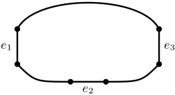
Step 3. For each q-cycle Cq ∈ CXε \ B3, obtain a q-path Pq by deleting the edge xx′ ∈ Cq such that δYε (x) + δYε (x′ ) - nεw(x, x′ ) minimized. Then, patch all paths into a single cycle C arbitrarily, and select the cycle into the packing.
An illustration of the patching operation in Step 3 can be seen in Figure 3. Moreover, it is easy to see that the length of each cycle in C is divisible by 3, and the algorithm takes O(n3 ) time, dominated by computing the minimum cycle packing CXε [Hartvigsen, 1984].
Theorem 10 (*). There is a O(n3 )-time algorithm to get a 3-path packing PXε in G[Xε] and a 3-path packing PYε in G[Yε] with δYε (PXε ) + nεw(PXε ) ≤ δYε (Xε) + 1 2 nεw(CXε ) and δXε (PYε ) + nεw(PYε ) ≤ δXε (Yε) + 1 2 nεw(CYε ).
Theorem 11. For BTTP with any n and any constant ε > 0, there is a randomized (3/2 + ε)-approximation algorithm with a running time of O(n3 ).
Proof. By Theorem 10, we can get 3-path packings PXε in G[Xε] and PYε in G[Yε] in O(n3 ) time with δYε (PXε ) + nεw(PXε )+δXε (PYε )+nεw(PYε ) ≤ δYε (Xε)+ 12 nεw(CXε ) +δXε (Yε) + 12 nεw(CYε ).
If n ≥ 108d3 , by Lemma 2 and Theorem 8, we can obtain a solution in O(n2 ) time with an expected weight of at most (3/2 + ε) · OPT by calling PXε and PYε on our randomized construction algorithm. Otherwise, as mentioned, we have n < 108d3 = Oε(1), and in this case, we can solve the problem optimally in constant time. Therefore, there is a randomized (3/2 + ε)-approximation algorithm for BTTP, and the total running time is O(n3 ).
Our algorithm is randomized because it uses a simple randomized labeling technique. It can be derandomized in polynomial time using the well-known method of conditional expectations in [Williamson and Shmoys, 2011], while preserving the approximation ratio.
6 Application
To test the performance of our algorithm, we introduce a new BTTP instance, and apply our algorithm to this instance. Additionally, we extend our construction to a 3-cycle construction by slightly modifying the design of normal super-games, which turns out to be more practical.
The New Instance. The construction of our instance is motivated by the real situation of NBA. Since 2004, the number of teams in NBA has always been 30, where there are 15 teams in the Western Conference and 15 teams in the Eastern Conference. Thus, Hoshino and Kawarabayashi [2011b] constructed an NBA instance with n = 15 for BTTP. In recent years, there have been rumors saying that NBA is poised to expand to 32 teams in 2024, with the potential inclusion of two new teams from Las Vegas and Seattle. Therefore, we create an instance, where we assume that two new teams from Las Vegas and Seattle join in the Western Conference, and also the Minnesota Timberwolves, originally from the Western Conference, are moved to join the Eastern Conference. This is an instance for BTTP with n = 16. We determined their distance matrix using the following method: first, we surveyed the home venues of the existing 30 teams and made educated guesses about the home venues of the two new teams; then, we obtained the longitude and latitude coordinates of these home venues using Google Maps; last, we calculated the distances (in miles) between any pair of teams based on the coordinates using the Haversine formula.
The Parameters. We set d = 1 and m = 5. Then, we have l = 1, and the games in the last time slot may violate the norepeat constraint. As in the proof of Theorem 7, if we denote the games on 2n days in our construction as g1g2 . . . g2n, we can rearrange them as g2ng1g2 . . . g2n-1 to fix this problem.
The 3-cycle Construction. Our construction can be easily extended to pack 3-cycles. We can modify our normal supergames as follows. Assume that there is a normal super-game between S = {s0, s1, s2} and T = {t0, t1, t2}. In the extension, we define mi := {si′ → t(i′+i) mod 3}2i′=0 , and arrange games on 6 days in the order of m0m1m2m0m1m2.
In the extension of the new normal super-game, each team in S (resp., T) plays 3-consecutive away games along two edges in the 3-cycle t0t1t2t0 (resp., s0s1s2s0). Moreover, on each day teams in the same league either all play home games or all play away games. Due to this, before extending one new normal super-game between super-teams S and T, we may relabel teams in S and teams T . There are 3!×3! = 36 ways, and we choose the best one so that the total traveling distance of teams in S ∪ T is minimized on the extended 6 days. We will recover their labels after extending the new normal supergame, and the feasibility still holds. Note that this property does not hold for the previous normal super-game.
Optimizing Left Super-games. The design of left supergames in our construction can be optimized. Recall that we arrange the games in left super-game as m1m2m3m1m2m3. To reduce the frequency of returning homes, we rearrange them as m1m2m3m1m3m2 for the 3-path construction, and m1m2m3m1m2m3 for the 3-cycle construction. The feasibility also holds.
The Implementations. Instead of finding a 3-path packing using the algorithm in Theorem 10, we directly label teams randomly, and try to improve our schedule by exchanging the labels of two teams in the same league. There are (n2 ) pairs of teams in X and (n2 ) pairs of teams in Y . We consider these n(n-1) pairs in a random order. From the first pair to the last, we test whether the weight of our schedule can be reduced after we swap the labels of teams in the pair. If no, we do not swap them and go to the next pair. If yes, we swap them and go to the next pair. After considering all the n(n - 1) pairs, if there is an improvement, we repeat the whole procedure. Otherwise, the procedure ends. Since the size of instance is small, it is sufficient to obtain a good solution very quickly.
| Construction | Result | Gap | Time |
|---|---|---|---|
| 3-path | 817086.814 | 24.66% | 0.85s |
| 3-cycle | 717172.797 | 9.42% | 1.03s |
Our algorithms are coded in C++, on a standard desktop computer with a 3.20GHz AMD Athlon 200GE CPU and 8 GB RAM.
The details of the new instance and our algorithms can be found in https://github.com/JingyangZhao/BTTP.
We compare our results with the well-known Independent Lower Bound [Easton et al., 2002]. The idea is to compute the best-possible traveling distance of a single team v (i.e., the traveling distance of its minimum weight itinerary) independently without considering the feasibility of other teams. The value is denoted as ILBv, and then the independent lower bound is ILB = ∑v∈X∪Y ILBv. Note that ILBv can be obtained by solving the Capacitated Vehicle Routing Problem (CVRP). For example, if v ∈ X, we obtain an instance of CVRP, where there is a vehicle with a capacity of 3 at v, each team in Y has a unit demand, and we need to find a minimum itinerary for the vehicle to fulfill the demand of teams in Y . To solve this instance of CVRP, we use a brute-force enumeration since the size is small. We have ILB = 655475.788.
Our results can be seen in Table 4, where the column 'Construction' indicates the 3-path and the 3-cycle constructions; 'Result' lists the results of our algorithms; 'Gap' is defined to be Result - ILB ILB , and 'Time' is the running time of our algorithms. We can see that both of our algorithms run very fast. Compared to ILB, the quality of the 3-path construction has a gap of 24.66%, which is much smaller than the expected 1.5-approximation ratio. Moreover, the 3-cycle construction is more practical, which can reduce the gap to only 9.42%.
7 Conclusion
In this paper, for BTTP with any n and any constant ε > 0, we propose a (3/2 + ε)-approximation algorithm, which significantly improves the previous result. Our theoretical result relies on three key ideas: the first is a new lower bound, the second is a new construction, and the third is a 3-path packing algorithm. Our methods also have the potential to design better approximation algorithms for TTP, which is left for future work. For applications, we create a new real instance from NBA for BTTP. Experimental results show that the 3-cycle construction has a very good practical performance.
Acknowledgements
This work is supported by National Natural Science Foundation of China under grants 62372095 and 62172077, and Natural Science Foundation of Sichuan Province of China under grant 2023NSFSC0059.
@inproceedings{ijcai2024p753,
  title     = {A Better Approximation for Bipartite Traveling Tournament in Inter-League Sports Scheduling},
  author    = {Zhao, Jingyang and Xiao, Mingyu},
  booktitle = {Proceedings of the Thirty-Third International Joint Conference on
               Artificial Intelligence, {IJCAI-24}},
  publisher = {International Joint Conferences on Artificial Intelligence Organization},
  editor    = {Kate Larson},
  pages     = {6814--6822},
  year      = {2024},
  month     = {8},
  note      = {Main Track},
  doi       = {10.24963/ijcai.2024/753},
  url       = {https://doi.org/10.24963/ijcai.2024/753},
}
TY - CPAPER TI - A Better Approximation for Bipartite Traveling Tournament in Inter-League Sports Scheduling AU - Zhao, Jingyang AU - Xiao, Mingyu T2 - Proceedings of the Thirty-Third International Joint Conference on Artificial Intelligence, IJCAI-24 PB - International Joint Conferences on Artificial Intelligence Organization PY - 2024 SP - 6814 EP - 6822 DO - 10.24963/ijcai.2024/753 UR - https://doi.org/10.24963/ijcai.2024/753 ER -Copied
Machine-readable versions of this paper, for tools and AI agents:





