Concentration Tail-Bound Analysis of Coevolutionary and Bandit Learning Algorithms

1 Introduction

Drift analysis is a powerful technique in understanding the performance of randomised algorithms, particularly in the field of runtime analysis of heuristic search. For more recent overviews of drift analysis in evolutionary computation, see [Doerr and Neumann, 2019; Neumann and Witt, 2010;

∗ Full version at https://arxiv.org/abs/2405.04480.

Jansen, 2013; He and Yao, 2001; Hajek, 1982]. The majority of existing drift theorems provide an upper bound on the expected runtime needed to reach a target state, such as an optimal solution set [He and Yao, 2001]. By identifying an appropriate potential function and demonstrating a positive drift towards the target state, the expected runtime can be bounded by the reciprocal of the drift multiplied by the maximum distance from the target state.

The focus of concentration tail-bound analysis is on quantifying the deviation of the runtime of randomised algorithm T, from its expected value. By providing insights into the distribution of T, this approach offers a more detailed understanding of an algorithm's performance [K¨otzing, 2016; Lehre and Witt, 2021; Doerr and Goldberg, 2013]. The concentration tail-bound analysis has gained significant interest due to its potential for delivering tighter upper bounds on the runtime of various algorithms. For instance, an exponential tail bound is used to bound the expected runtime of RLS on separable functions [Doerr et al., 2013]. Moreover, in the case of (1+1)-cooperative co-evolutionary algorithms, concentration tail-bound analysis can establish a Θ(n log(n)) bound for the runtime of the cooperative coevolutionary algorithm on linear functions [Lehre and Lin, 2023]. The concentration tail-bound analysis is also useful in the context of restarting arguments; for example [Case and Lehre, 2020]. More precise runtime estimation can be valuable in optimising and comparing different algorithms, potentially leading to improved algorithm design and performance [Bian et al., 2020; Dang et al., 2021; Zheng et al., 2022; Doerr and Qu, 2023].

Concentration tail bounds are not only used in runtime analysis to help us understand evolutionary algorithms, including simple genetic algorithms or coevolutionary algorithms [K¨otzing, 2016; Lehre and Lin, 2023], but can also be used in regret analysis of reinforcement learning algorithms. A typical example is using concentration inequality (AzumaHoeffding inequality) to provide precise bounds for regret. Concentration inequalities are used in the development of optimal UCB family algorithms, incorporating the concept of optimism in the face of uncertainty [Auer et al., 2002].

1.1 RelatedWork

Researchers use drift analysis to analyse not only the runtime of evolutionary algorithms but also other randomised algorithms like Random 2-SAT [G¨obel et al., 2022] or the expected regret of simple reinforcement learning algorithms on bandit problems [Larcher et al., 2023]. We would like to explore more advanced drift analysis tools to provide more precise estimates of runtime and regret. Various extensions of drift theorems have been proved, including multiplicative drift [Doerr et al., 2010], variable drift [Baritompa and Steel, 1996; Johannsen, 2010; Mitavskiy et al., 2009], and negative drift [Oliveto and Witt, 2012]. The multiplicative drift theorem [Doerr et al., 2010] refines the original additive drift theorem by considering the current state, resulting in a more precise bound when using the same potential function. Variable drift [Baritompa and Steel, 1996; Johannsen, 2010; Mitavskiy et al., 2009] generalises the multiplicative drift concept to incorporate an increasing positive function, h. On the other hand, negative drift [Oliveto and Witt, 2012] is employed to provide a lower bound for the expected runtime, often used to demonstrate that an algorithm has an exponential expected runtime, thereby proving its inefficiency.

In recent years, researchers have been exploring advanced drift theorems that focus on the tail bound of the runtime [K¨otzing, 2016; Lehre and Witt, 2021; Doerr and Goldberg, 2013]. Researchers are also interested in the applications of concentration inequalities, like the Azuma-Hoeffding inequalities [Azuma, 1967]. They provide deeper insights into the behaviour and performance of randomised algorithms [Doerr and K¨unnemann, 2013].

1.2 Our Contributions

This paper provides a novel perspective on analysing tail bounds by introducing a classic recurrence strategy. With the help of the recurrence strategy, this paper presents a sharper bound for all possible drift cases with a simpler proof. In particular, we provide an exponential tail bound under constant variance with negative drift. Refining an existing method, we also show a more precise exponential tail bound for the traditional cases with additive drift and for the cases in which there is constant variance but weak or zero drift.

Finally, we illustrate the practical impact of our findings by applying our theorems to various algorithms. The analysis brings us stronger performance guarantees for these algorithms. In particular, we prove the instability of the co-evolutionary algorithm (CoEA) on maximin optimisation (BILINEAR problem instance) occurs with high probability. Moreover, we show that the randomness of the reinforcement learning algorithm RWAB can help to find the optimal policy for the 2-armed non-stationary bandit problem with high probability. This paper is the first tail-bound analysis of both random local search with pairwise dominance (RLS-PD) and the bandit learning algorithm RWAB.

2 Preliminaries

For a filtration Ft, we write Et(·) := E(· | Ft). We denote the 1-norm as |z|1 = ∑ni=1 zi for z ∈ {0, 1}n and 1E by indicator function, i.e. 1E = 1 if event E holds and 0 otherwise. With high probability," will be abbreviated as "w.h.p.". We say an event En with problem size n ∈ N occurs w.h.p. if Pr(En) ≥ 1 - 1/poly(n). We defer pseudo-codes of algorithms and tables in the appendix.

We define the k-th stopping time, also called k-th hitting time, which will be used in later proofs.

Definition 1. (k-th stopping time) Given a stochastic process (Xt)t≥0 on a state space in R. Let the target set A be a finite non-empty subset of R, and then for any k ≥ 0, we define Tk = min{t ≥ k | Xt ∈ A}. In particular, T0 is the first hitting time at A.

We first provide a formal definition of variance-dominated and variance-transformed processes.

Definition 2. (Variance-dominated processes) A sequence of random variables X0,X1, · · · ∈ [0, n] is a variancedominated process with respect to the filtration F0,F1, . . . if for all t ∈ N, the following conditions hold:

Definition 3. (Variance-transformed processes) A sequence of random variables X0,X1, · · · ∈ [0, n] is a variancetransformed process with respect to the filtration F0, F1, . . . if for all t ∈ N, the following conditions hold:

This paper mainly focuses on random processes which consist of positive, weak (almost zero) or even a small negative drift with a constant second moment since these processes exhibit more complicated dynamics [K¨otzing et al., 2015; Friedrich et al., 2016; G¨obel et al., 2022; Doerr and Zheng, 2020]. A general polynomial tail bound is provided for these in [K¨otzing, 2016], but any general exponential tail bounds for these processes are still missing.

In the following sections, we exploit the Optional Stopping Time Theorem to obtain our exponential tail bound. This theorem is crucial for proving the original additive drift theorem, as highlighted by [He and Yao, 2001]. This recurrence method can provide a different perspective to derive the exponential tail bound in runtime analysis. We defer the statements of Optional Stopping Time Theorems in the appendix.

2.1 Previous Works and Discussion

With the development of runtime analysis, researchers have established several concentration tail bounds for EAs. For example, [Lehre and Witt, 2021] provides an exponential tail bound for the basic (1+1)-EAs on OneMax functions, which is a well-studied benchmark function to analyse the performance of EAs. To the best of our knowledge, the current best general tail bounds for both processes under the additive drift and variance-dominated processes can be found in [K¨otzing, 2016; Lehre and Witt, 2021].

[K¨otzing, 2016] shows that the runtime is at most quadratic in n with probability 1 - p for any p > 0. If we replace 1/pℓ log(c) by r > 0 and rewrite it in terms of an upper tail bound, then the original bound becomes that given two constants 1 ≤ c < n, ℓ > 0 and for any r > 0,

Although we have established a tail bound for variancedominated processes that concentrate on the expectation in a polynomial order with respect to r in Equation (1), it is worth exploring whether a more precise concentration tail bound can be derived for such processes, such as an exponential tail. A sharper exponential tail bound can improve the expected runtime estimation and thus provide useful insights into randomised algorithms.

3 ARecurrent Method in Upper Tail Bound

Next, we explore how to derive a general framework for providing exponential tail bound for randomised algorithms, including evolutionary algorithms which satisfy certain conditions. We explore the exit time of Xt out of some interval [0, b], using the same set-up as [K¨otzing, 2016].

In the proof of McDiamid inequality, [McDiarmid, 1989] also uses the Hoeffding lemma and conditions on the past events to establish the recurrence. [Doerr and Goldberg, 2013] uses the multiplicative drift condition directly to build up the exponential recurrence relation and hence obtain an exponential tail bound. We want to borrow these ideas to derive an exponential tail bound for variance-dominated processes. To do this, we introduce the k-th hitting time of the target state, which is also used in the theorem (Theorem 2.6.2) of [Menshikov et al., 2016]. We combine this recurrent method with the extended Optional Stopping Time theorem.

3.1 Variance Overcomes Negative Drift W.H.P.

We proceed to prove our main theorem by considering the most general variance drift theorem which overcomes some negative drift. Following the setting of [Hevia Fajardo et al., 2023], in variance-transformed cases, we focus on the first hitting time of a discrete-time stochastic process Xt at 0 given that Xt ∈ [0, b]. The proof of Theorem 1 uses Lemma 1.

Lemma 1. Let (Xt)t≥0 be random variables over R≥0, each with finite expectation. Let T be any stopping time of Xt. If there exist constants r, η > 0 with respect to j, t such that for any j ≥ 0, E(1{T>t}1{|Xt-Xt+1|≥j} | Ft ) ≤ r/(1 + η)j , then there exists a positive constant c such that E(|Xt+1 -Xt| · 1{T>t} | Ft ) ≤ c for all t ∈ N ∪ {0}.

By using Lemma 1, we now satisfy condition (4) in the Optional Stopping Time Theorem, enabling us to proceed with the main proof (details in the appendix). Utilising the extended Optional Stopping Time Theorem, we follow a classic approach for generalisation, which also frees us from the fixed step size condition and the need for the AzumaHoeffding inequality for sub-Gaussian supermartingales. 1 We further construct a new stochastic process Yt = b2 - (b - Xt)2 + δt, connected to the original process and the variance of the drift. By employing the idea of the k-th hitting time from [Menshikov et al., 2016], we obtain the upper bound for the k-th hitting time, allowing us to construct the recurrence. We present the main theorem of this paper.

1 The proofs in [K¨otzing, 2016] mainly rely on Azuma-Hoeffding inequality for sub-Gaussian supermartingales.

Theorem 1. Let (Xt)t∈N be a sequence of random variables in a finite state space S ⊆ R adapted to a filtration (Ft)t∈N, and let T = inf{t ≥ 0 | Xt ≤ 0}. Suppose

(A1) there exist δ > 0 such that for all t < T, it holds that

(A2) and for all t ≤ T , it holds that 0 ≤ Xt ≤ b.

Moreover, for all t ≥ 0, assume there exist constants r, η > 0 with respect to j, t, for any j ≥ 0, E(1{T>t}1{|Xt-Xt+1|≥j} | Ft ) ≤ r/(1+ η)j . Then, for τ > 0, Pr(T > τ ) ≤ e-τδ/eb2 .

Our main result (Theorem 1) allows the increased tolerance of negative drift rather than non-negative drift tendency and only necessitates a constant second moment of drift, instead of variance, as outlined in [K¨otzing, 2016]. Consequently, we can establish a more precise exponential tail bound for stochastic processes with a constant second moment of the drift, even under weak, zero, or negative drift.

3.2 Standard Variance Drift

This section presents the standard variance drift scenario (Theorem 2) as a corollary of Theorem 1. More precisely, we now restrict to the non-negative drift tendency. We first define several conditions which will be used later.

• (C1*) There exist constants r, η > 0 with respect to j, t, such that for any j ≥ 0 and for all t ≥ 0,

• (C1) There exists a constant c > 0 such that |Xt-Xt+1| < c for all t ≥ 0.
• (C2) E(Xt+1 -Xt | Ft) ≥ 0 for all t ≥ 0.
• (C3) There exists some constant δ > 0 such that E(Xt+1 -Xt)2 | Ft ) ≥ δ for all t ≥ 0.

Theorem 2. Let (Xt)t≥0 be random variables over R≥0, each with finite expectation, such that conditions (C1∗ ), (C2) and (C3) hold. For any b > 0, define T = inf{t ≥ 0 | Xt ≥ b}. If X0 ∈ [b], then E(T) ≤ (b2 -X2 0 )/δ. Moreover, for τ > 0, Pr(T ≥ τ ) ≤ e-τδ/eb2 .

Theorem 2 tells us that under the standard variance drift case as discussed in [K¨otzing, 2016], we can derive an exponential tail bound for the runtime and such a process exhibits a high concentration around the expectation.

Now, we present a corollary which consists of the fixed step size condition.

Corollary 3. Let (Xt)t≥0 be random variables over R≥0, each with finite expectation which satisfy conditions (C1), (C2) and (C3). For any b > 0, define T = inf{t ≥ 0 | Xt ≥ b}. Given that X0 ∈ [0, b], then E(T) ≤ (b2 -X2 0 )/δ. Moreover, for τ > 0, Pr(T ≥ τ) ≤ e-τδ/eb2 .

Furthermore, we derive a tail bound for the variancedominated processes with two absorbing states. Following the setting of Theorem 10 in [G¨obel et al., 2022], we will prove the next theorem.

Theorem 4. Let (Xt)t≥0 be random variables over R≥0, each with finite expectation such that (C1∗), (C3) and E(Xt+1 -Xt | Ft) = 0 hold. For any b > 0, define T = inf{t ≥ 0 | Xt ∈ {0, b}}. If X0 ∈ [0, b], then E(T ) ≤ (X0(b - X0))/δ.

This proof is similar to Theorem 1 except that we use a different stochastic process Yt = Xt(b - Xt) + δt and show that Yt is a super-martingale. Unlike the proof of Theorem 1, the proof of Theorem 4 uses the extended Optional Stopping Time Theorem for super-martingale [Williams, 1991]. We defer the proof to the appendix.

3.3 Standard Drift

If a stochastic process has drift ε where ε > 0 is some positive constant, then we can give a different proof for the upper tail bound for additive drift from the proof in [K¨otzing, 2016]. This provides a more precise exponential upper tail bound.

Theorem 5. Let (Xt)t≥0 be random variables over R, each with finite expectation which satisfy condition (C1∗) and E[Xt+1 - Xt | Ft] ≥ ε for some ε > 0. For any b > 0, define T = inf{t ≥ 0 | Xt ≥ b}. If X0 ∈ [0, b], then E(T) ≤ b-X0 ε . Moreover, for τ > 0, Pr (T ≥ τ) ≤ e-τε/eb .

We recover the exponential upper tail bound for the additive drift theorem. The bound we obtain gets rid of the coefficients 1/8c2 in [K¨otzing, 2016]. Theorem 2.5.12 of [Menshikov et al., 2016] provides a similar result and uses a similar recurrence proof idea. While our result generalises the result in [Menshikov et al., 2016] by releasing the fixed step size, we provide a meaningful bound on the first hitting time instead of bounding it above by infinity.

In summary, we have discovered a simple alternative to the Azuma-Hoeffding inequality that provides an exponential tail bound by only relying on basic martingale theory. This result can be applied to the random local search (RLS) type algorithms that make finite steps at each iteration, as well as other randomised algorithms including evolutionary algorithms (EAs) that account for the possibility of large jumps occurring. Another benefit from Theorem 1 is that it allows the tolerance of the negative drift up to -Ω(1/b).

4 Applications to Random 2-SAT and Graph Colouring

In this section, we illustrate our theorems on practical examples. We consider the examples provided by [McDiarmid, 1993; Mitzenmacher and Upfal, 2005; G¨obel et al., 2022]. which include variance-dominated processes. We first discuss the Random 2-SAT problem.

4.1 Applications to Random 2-SAT

The 2-SAT Algorithm is designed to solve instances of the 2SAT problem, where a formula consists of clauses and each of them contains exactly two literals (either variables or negations). In each iteration, the algorithm selects an unsatisfied clause and picks one of the literals uniformly at random. The truth value of the variable corresponding to this literal is then inverted. Repeat the process until either we meet the stopping criteria or a valid truth assignment is found.

[Papadimitriou, 1991] firstly provided a time complexity analysis on such a simple randomised algorithm that returns a satisfying assignment of a satisfiable 2-SAT formula ϕ with n variables. Later, [G¨obel et al., 2022] recovered the results using drift analysis tools which we put in the Appendix.

By applying Theorem 2 with a variance bound 1, we can bound the number of function evaluations of order O(n4 ) with an upper exponential tail bound.

Theorem 6. Given any r ≥ 0, the randomised 2-SAT algorithm, when run on a satisfiable 2-SAT formula over n ∈ N variables, terminates in at most rn4 time with probability at least 1 - e-r/e .

4.2 Applications to Graph Colouring

Now we consider graph colouring, which has already been studied by [McDiarmid, 1993] and [G¨obel et al., 2022]. The recolour algorithm generates a 2-colouring mapping with the condition that no monochromatic edges can be found. The algorithm assumes a subroutine called SEEK, which, given a 2-colouring of the points, outputs a monochromatic edge if one exists. If there are no monochromatic edges, then the algorithm terminates. Otherwise, the algorithm repeats picking a point uniformly at random from the given monochromatic edge and changes its colour.

[G¨obel et al., 2022] provided a simpler proof of the O(n4 ) expected runtime of the recolouring algorithm for finding a 2-colouring with no monochromatic triangles on 3-colorable graphs. Following the setting and the proof of [G¨obel et al., 2022], by using Theorem 4, we can derive the following:

Theorem 7. Given any r ≥ 0, the randomised Recolouring algorithm on a 3-colorable graph with n ∈ N vertices over n ∈ N variables, terminates in at most rn4 time with probability at least 1- e-4r/3e .

5 Applications to Coevolutionary Algorithms

Next, we consider a slightly complicated example: competitive co-evolutionary algorithms (CoEAs). Competitive coevolutionary algorithms are designed to solve maximin optimisation or adversarial optimisation problems, including two-player zero-sum games [Popovici et al., 2012; Lehre, 2022]. There are various applications, including CoEA-GAN [Toutouh et al., 2019], competitive co-evolutionary search heuristics on cyber security problem [Lehre et al., 2023] and enhanced GANs by using a co-evolutionary approach for image translation [Shu et al., 2019].

We are interested in whether competitive CoEAs can help find Nash equilibrium efficiently. We use the formulation in [Nisan et al., 2007] to define Nash equilibrium. This paper focuses on Pure Strategy Nash Equilibrium (abbreviated NE).

Definition 4. ([Nisan et al., 2007]) Consider a two-player zero-sum game. Given a search space X × Y and a payoff function g : X ×Y →R, if for all (x, y) ∈ X ×Y

then (x∗ , y∗ ) is called a Pure Strategy Nash Equilibrium of a two-player zero-sum game.

The pairwise dominance relation has been defined and introduced into a population-based CoEA in [Lehre, 2022].

Definition 5 (Pairwise dominance). Given a function g = X × Y → R and two pairs (x1, y1), (x2, y2) ∈ X × Y, we say that (x1, y1) dominates (x2, y2) with respect to g, denoted (x1, y1) ⪰g (x2, y2), if and only if g(x1, y2) ≥ g(x1, y1) ≥ g(x2, y1).

There is a single-pair CoEA called Randomised Local Search with Pairwise Dominance (RLS-PD) [Hevia Fajardo et al., 2023]. It has been shown that RLS-PD can find the NE of a simple pseudo-Boolean benchmark called BILINEAR in expected polynomial runtime. The processes induced by RLS-PD on the BILINEAR problem is exactly a variancetransformed process. We would like to use Theorem 1 to show the exponential tail bound for the runtime.

RLS-PD samples a search point (a pair of point (x1, y1) ∈ X ×Y) uniformly at random. In each iteration, RLS-PD uses the local mutation operator to generate the new search point where the local mutation operator is sampling a random Hamming neighbour. If the new search point dominates the original search point in a pairwise-dominance manner, then the original search point is replaced by the new one. Otherwise, the original search point remains the same.

5.1 The BILINEAR Problem

In this section, we consider a simple class of discrete maximin benchmark called BILINEAR, which was first proposed by [Lehre, 2022]. In this work, we use a variation of BILINEAR as [Hevia Fajardo et al., 2023] to simplify our calculation and illustrate applications of our main theorem. It has been empirically shown in [Hevia Fajardo et al., 2023] that RLS-PD behaves similarly on the original definition of BILINEAR and the revised definition. In this paper, we only consider this variation of BILINEAR.

Definition 6. ([Hevia Fajardo et al., 2023]) The BILINEAR function is defined for two parameters α, β ∈ (0, 1) by

BILINEARα,β(x, y) := |y|1 (|x|1-βn)-αn |x|1+E1+E2 with the error terms E1 := max{(αn - |y|1 )2 , 1}/n3 and E2 := -max{(βn - |x|1 )2 , 1}/n3 . We also denote the set of Nash equilibria as OPT, where OPT := {(x, y) | |x|1 = βn ∧ |y|1 = αn}.

We consider OPT as our solution concept and the problem setting α = 1/2 ± O(1/√n) and β = 1/2 ± O(1/√n) as in [Hevia Fajardo et al., 2023]. We now derive the exponential tail bound of RLS-PD to find the Nash equilibrium.

5.2 RLS-PD Solves BILINEAR EfficientlyW.H.P.

Theorem 8. Consider α ∈ [1/2 - A/√n, 1/2 + A/√n] and β ∈ [1/2 - B/√n, 1/2 + B/√n], where A,B > 0 are constants and 3(A+B)2 ≤ 1/2 - δ′ for some constant δ′ > 0. The expected runtime of RLS-PD on BILINEARα,β is O(n1.5 ). Moreover, given any r ≥ 0, the runtime is at most 2rn1.5 , with probability at least 1 - e-Ω(r) .

We defer the proof of Theorem 8 to the appendix.

Theorem 8 shows that RLS-PD can find the Nash Equilibrium in O(n1.5 ) with overwhelmingly high probability. The exponential tail bound provides a stronger performance guarantee up to the tail of the runtime than the sole expectation.

5.3 RLS-PD Forgets the Nash EquilibriumW.H.P.

After the algorithm finds a Nash Equilibrium efficiently, the inherent characteristics of the function cause the algorithm not only to forget the Nash Equilibrium but also move away from it by a distance Ω(√n) in O(n) iterations w.h.p. This is shown by the following theorem.

Theorem 9. Let α = 1/2 ±A/√n and β = 1/2 ±B/√n, where A,B > 0 are constants. Consider RLS-PD on BILINEARα,β. Then, for any initial search points (x0, y0), the expected runtime that the search point firstly moves away from OPT by a Manhattan distance at least (A + B)√n is O(n). Moreover, given any r > 0, the runtime is at most rn, with probability at least 1 - e-Ω(r) .

Theorem 9 illustrates how drift analysis can expose weaknesses in algorithms, suggesting what needs to be improved in new algorithms. In particular, we can see even though RLS-PD can find the optimum in polynomial time, it can still suffer from evolutionary forgetting (i.e. forget the optimum found in previous iterations) with high probability. So only the expected runtime estimate might be insufficient to determine whether a coevolutionary algorithm is good or not. This highlights the weakness of RLS-PD and the need to understand coevolutionary dynamics further.

6 Applications to Regret Analysis of a Bandit Learning Algorithm

We start with a brief introduction of bandit problems. Suppose we have K decisions or "arms", where we obtain the corresponding reward ra when we choose one specific decision a. The goal of the bandit algorithm is to maximise cumulative reward among time horizon T [Lattimore and Szepesv´ari, 2020; Sutton and Barto, 2018]. In this paper, we consider the quantity called regret (missed reward), which is the difference between the reward of the chosen arm and the optimal arm at each iteration. We provide a formal definition of regret as follows.

Definition 7. ([Lattimore and Szepesv´ari, 2020; Larcher et al., 2023]) Given time horizon T, each arm a is associated with a probability distribution D(a), which we assume to be over [0, 1] and for which the mean is denoted as µ(a); whenever arm a is pulled, the agent receives a reward distributed according to D(a). The regret (missed reward) of the agent at round t ∈ N is defined as Rt = ra∗ - rat , where at is the arm chosen at round t, ra is the reward obtained from reward distribution D(a) and a∗ = arg max{µ(a) | a ∈ [K]}. The goal of the agent is to minimise the total regret R = ∑Tt=1 Rt or the total expected regret E(R).

This paper focuses on the non-stationary 2-armed bandit problem, in which the reward distributions may swap over time and K = 2. More precisely, the agent receives a reward according to a reward distribution D(a1) by pulling arm a1 and another reward according to another reward distribution D(a2) by pulling arm a2. We assume that two distributions D(a1) and D(a2) are fixed, and they will swap if a change occurs along the time horizon. To simplify the calculation, we assume both distributions over [0, 1]. We present the application of our drift theorem (concentration tail bound) on regret analysis of a simple reinforcement learning algorithm for such a bandit problem. We defer the pseudo-code for Random Walk with Asymmetric Boundaries (RWAB) proposed by [Larcher et al., 2023] to the appendix.

Note that RWAB is designed to balance the exploration and exploitation for non-stationary bandit problems. RWAB mainly relies on the CHALLENGE operator to determine which arm we prefer to pull or whether we swap the arms. The CHALLENGE operator is designed to use the random walk of action value S on [-√T/L, 1]. [Larcher et al., 2023] shows that the expected regret of RWAB is Θ (√LT ) where T is the time horizon and L is the number of changes. We want stronger performance guarantees for the regret of RWAB, i.e. a concentration tail bound for the regret estimate. We would like to characterise the distribution of the regret.

Next, we present the main theorem for the regret of RWAB algorithm. In this theorem, we assume L = o(T).

Theorem 10. Given any ε ≥ 1, the regret of Algorithm RWAB is at most 480ε(L + √LT) with probability at least 1 - 2e-√ε/e .

The proof of Theorem 10 is deferred to the Appendix. By Theorem 10, RWAB Algorithm has regret at most order O (√LT ) for a 2-armed non-stationary bandit problem w.h.p. By using minimax lower bound [Bubeck et al., 2012], any algorithm on K-armed stationary bandit problems has regret at least √Kn/20 for time horizon n. In particular, for K = 2, the lower bound for the expected regret of any algorithm on bandit stationary bandit problems is Ω(√n) for time horizon n. [Larcher et al., 2023] showed that by considering L changes and each change of average steps T/L, RWAB has expected regret at least Ω (L · √T/L) = Ω (√LT ). Theorem 10 confirms that RWAB is optimal with overwhelmingly high probability, and we propose a new perspective of analysing a bandit algorithm by using drift analysis, which is rarely employed by the reinforcement learning community.

7 Experiments

To complement our asymptotic results with data for concrete problem sizes, we conduct the following experiments.

7.1 Empirical Evidence of RLS-PD on BILINEAR

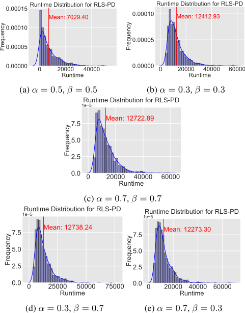
We conduct experiments with the RLS-PD for the maximin BILINEAR problem. The problem setup is (α, β) = (0.5, 0.5), (0.3, 0.3), (0.3, 0.7), (0.7, 0.3), (0.7, 0.7). These five scenarios cover the cases when the optimum lies in four different quadrants and the centre of the search space. We set the mutation rate χ = 1 and problem size n = 1000. We run 1000 independent simulations for each configuration. For each run, we initialise the search point uniformly at random.

Figure 1 displays the density plot for the runtime distribution of RLS-PD on BILINEAR. The x-axis represents the runtime, the y-axis represents the frequency or density, and the red dotted line represents the average value of the runtime for each problem setting. As x increases, Figure 1 shows that we have an exponentially decaying tail for the runtime of RLS-PD on each problem configuration. It is very unlikely that the runtime of RLS-PD on BILINEAR deviates too much from the mean or the expected runtime from Figure 1 for each problem configuration. From the statistics (figures and tables in the appendix), we can see for each configuration, the frequency that the actual runtime bounded above by the mean runtime converges to 1. When (α, β) = (0.5, 0.5), the empirical results are consistent with our theoretical bounds in the sense of asymptotic order. The results for other problem configurations raise a conjecture about whether our theoretical results can also hold for all α, β ∈ [0, 1].

7.2 Empirical Evidence of RWAB Algorithm

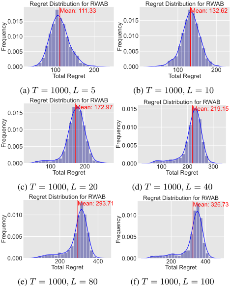
We conduct experiments with the RWAB Algorithm for the 2-armed non-stationary bandit problem. The environment is set up as two Bernoulli bandits with means µ1 = 0.2, µ2 = 0.8 and the number of changes L = 5, 10, 20, 40, 80, 100. The changes are set up uniformly at random along the time horizon T = 1000. 1000 independent simulations are run for each configuration.

Figure 2 displays the regret distribution of RWAB. The xaxis represents the regret of RWAB, the y-axis represents the frequency or density, and the red dotted line represents the average regret for each problem setting. As x increases, Figure 2 shows that we have an exponentially decaying tail for the regret of RWAB on 2-armed non-stationary bandit problem with respect to the changes L. Figure 2 shows the concentration of regret around the empirical mean or the expected regret and it is also unlikely that the regret of RWAB deviates too much from the expectation. The tables (deferred in the appendix) suggest that our theoretical tail bound is asymptotically tight regardless of the leading coefficient. Tables and figures for regret distributions show that for each configuration, the frequency that the actual regret bounded above by the mean regret is asymptotic to 1 as the increases in the multiplicative factors of the upper bounds. Moreover, the convergence rate is significantly faster than the counterpart in the case of RLS-PD on BILINEAR. This means that the theoretical bound (i.e. the leading coefficient) obtained has room to improve. One conjecture may be the process governing the dynamics of runtime for RLS-PD on BILINEAR relies heavily on the high variance needed to overcome the negative drift, while the process governing the dynamics of regret induced by RWAB already exhibits positive drift everywhere before reaching the target state. Thus, it yields a faster convergence.

8 Conclusion

This paper proves a more general and stronger drift theorem (tail-bound). Our theorems can be used to analyse the first hitting time of different random processes. As a sub-product, this paper also resolves the open problem left in [K¨otzing,

2016], which asks for a suitable replacement for the AzumaHoeffding inequality to improve the tail bounds for random processes. We apply our theorems to several practical examples, including Random 2-SAT, Recolouring, competitive CoEAs and RWAB. To the best of our knowledge, it is the first tail-bound drift analysis of RLS-PD and RWAB. Our drift theorems provide more precise information on how the runtime concentrates and a stronger performance guarantee. In practice, it shows the limitation of the current coevolutionary algorithm on maximin optimisation. It suggests a need for a deeper understanding of the mechanism of CoEAs, which may help to design a more stable CoEA. Moreover, our results confirm that randomness in RWAB can be helpful for stochastic non-stationary bandit problems.

For future studies, both runtime analysis of CoEA on maximin optimisation and regret analysis of stochastic reinforcement learning algorithms via drift analysis are still poorly understood and unexplored areas. In particular, on the technical side, can we derive more precise bounds for RWAB since the leading coefficient seems not to be optimal from empirical results or can we use these results to analyse more complicated CoEAs or bandit algorithms? On the practical side, we could try to use such concentration bound to design more efficient algorithms. For example, we could try to design more stable CoEAs or develop a general optimal bandit algorithm by using the random-walk design analysed in this work.

Acknowledgments

This work was supported by a Turing AI Fellowship (EPSRC grant ref EP/V025562/1). The computations were performed using the University of Birmingham's BlueBEAR high performance computing (HPC) service.

Contribution Statement

Authors are listed in alphabetical order.