
Exactly Solving Minimum Dominating Set and Its Generalization
Proceedings of the Thirty-Third International Joint Conference on Artificial Intelligence. Main Track. Pages 7056-7064.
https://doi.org/10.24963/ijcai.2024/780
Keywords
- Search: S: Combinatorial search and optimisation
Abstract
The Minimum Dominating Set Problem (MDSP) is an important NP-Hard optimization problem with many applications in various domains. This paper designs two exact algorithms for MDSP that use the same Branch-and-Bound framework. However, one uses LP relaxations as lower bounds for pruning the search space, and the other one is a pure combinatorial algorithm. The two algorithms possess a distinct advantage. Performance experiments on standard test datasets reveal that our combinatorial algorithm is over 1000 times faster than the previous state-of-the-art exact algorithm presented in IJCAI 2023, and our LP Relaxation algorithm can even enhance the speed of our combinatorial algorithm by over 100 times. However, our combinatorial algorithm still outperform the LP Relaxation algorithm on very dense graphs.
- Dataset: T1 |V | |E| BIBLP BIBCO BIBLP-IF BIBCO-IF EMOS 150 150 0.01 0.01 0.01 633.06(2) 25.03 150 250 0.03 1.41 0.03 28.02 334.58 150 500 8.18 2203.54(4) 10.46 1903.10(4) 2919.74(9) 150 750 11.17 2386.31(5) 12.37 1134.20(2) 3000.00(10) 150 1000 23.97 2224.23(4) 25.76 665.26(1) 3000.00(10) 150 2000 9.89 97.62 9.16 15.92 1851.73 150 3000 9.11 23.66 9.00 4.18 270.71 200 250 0.01 0.12 0.02 1840.26(5) 2900.47(7) 200 500 307.25(1) 2927.73(9) 18.07 3000.00(10) 3000.00(10) 200 750 166.89 3000.00(10) 200.27 3000.00(10) 3000.00(10) 200 1000 789.56 3000.00(10) 984.52 3000.00(10) 3000.00(10) 200 2000 1450.30 3000.00(10) 1559.50 3000.00(10) 3000.00(10) 200 3000 656.70 3000.00(10) 602.74 3000.00(10) 3000.00(10) 250 250 0.01 0.01 0.01 3000.00(10) 3000.00(10) 250 500 13.83 2783.49(9) 19.06 3000.00(10) 3000.00(10) 250 750 1030.34(1) 3000.00(10) 1054.77(1) 3000.00(10) 3000.00(10) 250 1000 2504.13(7) 3000.00(10) 2508.30(7) 3000.00(10) 3000.00(10) 300 300 0.01 0.01 0.01 3000.00(10) 3000.00(10) 300 500 5.80 2852.50(9) 5.36 3000.00(10) 3000.00(10) 300 750 1751.27(3) 3000.00(10) 2081.97(6) 3000.00(10) 3000.00(10) 800 1000 23.51 3000.00(10) 32.57 3000.00(10) 3000.00(
- [Alber et al., 2004] Jochen Alber, Michael R. Fellows, and Rolf Niedermeier. Polynomial-time data reduction for dominating set. J. ACM, 51(3):363-384, 2004.
- [Baïou and Barahona, 2014] Mourad Baïou and Francisco Barahona. The dominating set polytope via facility loca- tion. In Pierre Fouilhoux, Luis Eduardo Neves Gouveia, Ali Ridha Mahjoub, and Vangelis Th. Paschos, editors, Combinatorial Optimization -Third International Sympo- sium, ISCO 2014, Lisbon, Portugal, March 5-7, 2014, Re- vised Selected Papers, volume 8596 of Lecture Notes in Computer Science, pages 38-49. Springer, 2014.
- [Cai et al., 2020] Shaowei Cai, Wenying Hou, Yiyuan Wang, Chuan Luo, and Qingwei Lin. Two-goal local search and inference rules for minimum dominating set. In Christian Bessiere, editor, Proceedings of the Twenty-Ninth Inter- national Joint Conference on Artificial Intelligence, IJCAI 2020, pages 1467-1473. ijcai.org, 2020. IJCAI
- [Chaurasia and Singh, 2015] Sachchida Nand Chaurasia and Alok Singh. A hybrid evolutionary algorithm with guided mutation for minimum weight dominating set. Appl. In- tell., 43(3):512-529, 2015.
- [Courcelle, 1990] Bruno Courcelle. Graph rewriting: An al- gebraic and logic approach. In Jan van Leeuwen, editor, Handbook of Theoretical Computer Science, Volume B: Formal Models and Semantics, pages 193-242. Elsevier and MIT Press, 1990.
- [Cygan et al., 2011] Marek Cygan, Geevarghese Philip, Marcin Pilipczuk, Michal Pilipczuk, and Jakub Onufry Wojtaszczyk. Dominating set is fixed parameter tractable in claw-free graphs. Theor. Comput. Sci., 412(50):6982- 7000, 2011.
- [Dinh et al., 2014] Thang N. Dinh, Yilin Shen, Dung T. Nguyen, and My T. Thai. On the approximability of posi- tive influence dominating set in social networks. J. Comb. Optim., 27(3):487-503, 2014.
- [Ellis et al., 2004] John A. Ellis, Hongbing Fan, and Michael R. Fellows. The dominating set problem is fixed parameter tractable for graphs of bounded genus. J. Algo- rithms, 52(2):152-168, 2004.
- [Fan et al., 2019] Yi Fan, Yongxuan Lai, Chengqian Li, Nan Li, Zongjie Ma, Jun Zhou, Longin Jan Latecki, and Kaile Su. Efficient local search for minimum dominating sets in large graphs. In Guoliang Li, Jun Yang, João Gama, Jug- gapong Natwichai, and Yongxin Tong, editors, Database Systems for Advanced Applications -24th International Conference, DASFAA 2019, Chiang Mai, Thailand, April 22-25, 2019, Proceedings, Part II, volume 11447 of Lec- ture Notes in Computer Science, pages 211-228. Springer, 2019.
- [Garey and Johnson, 1979] Michael Randolph Garey and David Stifler Johnson. Computers and Intractability: A Guide to the Theory of NP-Completeness. W. H. Freeman & Co., 1979.
- [Gast et al., 2015] Mikael Gast, Mathias Hauptmann, and Marek Karpinski. Inapproximability of dominating set on power law graphs. Theor. Comput. Sci., 562:436-452, 2015.
- [Hassani Karbasi and Ebrahimi Atani, 2013] Amir Has- sani Karbasi and Reza Ebrahimi Atani. Application of dominating sets in wireless sensor networks. International Journal of Security and its Applications, 7:185-202, 01 2013.
- [Hedar and Ismail, 2010] Abdel-Rahman Hedar and Rashad Ismail. Hybrid genetic algorithm for minimum dominating set problem. In David Taniar, Osvaldo Gervasi, Beniamino Murgante, Eric Pardede, and Bernady O. Apduhan, edi- tors, Computational Science and Its Applications -ICCSA 2010, International Conference, Fukuoka, Japan, March 23-26, 2010, Proceedings, Part IV, volume 6019 of Lec- ture Notes in Computer Science, pages 457-467. Springer, 2010.
- [Huangfu and Hall, 2018] Qi Huangfu and Julian Hall. Par- allelizing the dual revised simplex method. Math. Pro- gram. Comput., 10(1):119-142, 2018.
- [Inza et al., 2024] Ernesto Parra Inza, Nodari Vakhania, José María Sigarreta Almira, and Frank Angel Hernández Mira. Exact and heuristic algorithms for the domination prob- lem. Eur. J. Oper. Res., 313(3):926-936, 2024.
- [Iwata, 2011] Yoichi Iwata. A faster algorithm for dominat- ing set analyzed by the potential method. In Dániel Marx and Peter Rossmanith, editors, Parameterized and Exact Computation -6th International Symposium, IPEC 2011, Saarbrücken, Germany, September 6-8, 2011. Revised Se- lected Papers, volume 7112 of Lecture Notes in Computer Science, pages 41-54. Springer, 2011.
- [Jiang and Zheng, 2023] Hua Jiang and Zhifei Zheng. An exact algorithm for the minimum dominating set problem. In Proceedings of the Thirty-Second International Joint Conference on Artificial Intelligence, IJCAI 2023, 19th- 25th August 2023, Macao, SAR, China, pages 5604-5612. IJCAI
- [Jovanovic et al., 2010] Raka Jovanovic, Milan Tuba, and Dana Simian. Ant colony optimization applied to mini- mum weight dominating set problem. pages 322-326, 05 2010.
- [Karp, 1972] Richard M. Karp. Reducibility among combi- natorial problems. In Raymond E. Miller and James W. Thatcher, editors, Proceedings of a symposium on the Complexity of Computer Computations, held March 20- 22, 1972, at the IBM Thomas J. Watson Research Cen- ter, Yorktown Heights, New York, USA, The IBM Research Symposia Series, pages 85-103. Plenum Press, New York, 1972.
- [Lin et al., 2016] Geng Lin, Wenxing Zhu, and M. Montaz Ali. An effective hybrid memetic algorithm for the mini- mum weight dominating set problem. IEEE Trans. Evol. Comput., 20(6):892-907, 2016.
- [Potluri and Singh, 2011] Anupama Potluri and Alok Singh. Two hybrid meta-heuristic approaches for minimum dom- inating set problem. In Proceedings of the Second Interna- tional Conference on Swarm, Evolutionary, and Memetic Computing -Volume Part II, SEMCCO'11, page 97-104, Berlin, Heidelberg, 2011. Springer-Verlag.
- [Potluri and Singh, 2013] Anupama Potluri and Alok Singh. Hybrid metaheuristic algorithms for minimum weight dominating set. Appl. Soft Comput., 13(1):76-88, 2013.
- [Raz and Safra, 1997] Ran Raz and Shmuel Safra. A sub- constant error-probability low-degree test, and a sub- constant error-probability PCP characterization of NP. In Frank Thomson Leighton and Peter W. Shor, editors, Pro- ceedings of the Twenty-Ninth Annual ACM Symposium on the Theory of Computing, El Paso, Texas, USA, May 4-6, 1997, pages 475-484. ACM, 1997.
- [Rossi and Ahmed, 2015] Ryan A. Rossi and Nesreen K. Ahmed. The network data repository with interactive graph analytics and visualization. In AAAI, 2015.
- [Sanchis, 2002] Laura A. Sanchis. Experimental analysis of heuristic algorithms for the dominating set problem. Algo- rithmica, 33(1):3-18, 2002.
- [Vazirani, 2001] Vijay V. Vazirani. Approximation algo- rithms. Springer, 2001.
- [Wang et al., 2017] Yiyuan Wang, Shaowei Cai, and Ming- hao Yin. Local search for minimum weight dominating set with two-level configuration checking and frequency based scoring function. J. Artif. Intell. Res., 58:267-295, 2017.
- [Wang et al., 2018] Yiyuan Wang, Shaowei Cai, Jiejiang Chen, and Minghao Yin. A fast local search algorithm for minimum weight dominating set problem on massive graphs. In Jérôme Lang, editor, Proceedings of the Twenty- Seventh International Joint Conference on Artificial Intel- ligence, IJCAI 2018, July 13-19, 2018, Stockholm, Swe- den, pages 1514-1522. ijcai.org, 2018. IJCAI
References were extracted automatically from the PDF and may contain errors.
Full text extracted automatically from the PDF; figures, tables and equations may differ. The PDF is the version of record.
1 Introduction
The Minimum Dominating Set Problem (MDSP) is a cornerstone in combinatorial optimization, with applications spanning social network analysis [Dinh et al., 2014], facility location [Ba¨ıou and Barahona, 2014], and wireless sensor networks [Hassani Karbasi and Ebrahimi Atani, 2013]. It aims to identify the smallest possible subset of vertices in a graph such that every vertex not in the subset is adjacent to at least one vertex within the subset.
MDSP is recognized as NP-complete [Karp, 1972; Garey and Johnson, 1979], implying that an efficient algorithm capable of solving it exactly for all graphs is unlikely. Using measure-and-conquer methods, Iwata proposed a branching algorithm that solves MDSP in O(1.4689n ) time and space on graphs with n vertices. In addition to these theoretical results, [Jiang and Zheng, 2023] developed a practical exact algorithm that solves MDSP on synthetic unit-disk graphs with up to 500 vertices within five hours. Their approach involved preprocessing the input graph using a reduction rule from [Alber et al., 2004], and designing a branch-and-bound algorithm based on a lower bound derived from independent sets on two-hop graphs. Quite recently, [Inza et al., 2024]
∗Contact Author
designed an implicit enumeration algorithm for MDSP based on binary searching the solution size and enumerating the vertices in the dominating set with priority.
Approximation algorithms offer a practical approach to complex problems where finding the exact solution may be too computationally expensive or time-consuming. While these algorithms may not always find the optimal solution, they provide solutions that are theoretically guaranteed to be within a certain ratio of the optimal solution. A simple greedy algorithm exists that solves MDSP with an approximation ratio of Hn, where Hn is the n-th harmonic number [Vazirani, 2001]. Assuming P ̸= NP, MDSP cannot be approximated within any constant factor [Raz and Safra, 1997]. This result was later improved by [Gast et al., 2015], who proved that MDSP cannot be approximated within an approximation ratio of Ω(ln n).
In terms of parameterized complexity, MDSP is considered intractable for the parameter k being the solution size. A problem is fixed parameter tractable (FPT) with respect to parameter k if there exists an algorithm that solves a problem instance of size n within O(poly(n)f(k)), where f is an arbitrary computable function. However, FPT algorithms for MDSP do exist for several graph classes, including graphs with bounded tree-width [Courcelle, 1990], graphs with bounded genus [Ellis et al., 2004], and claw-free graphs [Cygan et al., 2011].
Heuristic algorithms play a pivotal role in solving MDSP, especially when dealing with large-scale instances where exact algorithms may not be feasible. Over the past decades, due to the importance of MDSP in practical applications, a vast number of heuristic algorithms for MDSP have been developed. These include greedy algorithms [Sanchis, 2002], which are fast but often yield suboptimal solutions, metaheuristic algorithms that combine various search techniques [Hedar and Ismail, 2010; Jovanovic et al., 2010; Potluri and Singh, 2013; Chaurasia and Singh, 2015; Lin et al., 2016], and local search algorithms that start with an initial solution and progressively move towards better solutions [Wang et al., 2017; Wang et al., 2018; Fan et al., 2019; Cai et al., 2020]. These heuristic methods have been successfully applied to solve DSP and its variants, providing good solutions within a reasonable time frame.
Our contribution This paper presents a comprehensive study of exact methods for MDSP. Indeed, we will consider a more general problem EMDSP, where some vertices in the graph are not required to be dominated and some vertices are not allowed to be selected to the solution set to dominate other vertices. We introduce two novel branch-and-bound algorithms for EMDSP, incorporating several simple yet effective techniques. Both of the two algorithms utilize the same set of three reduction rules. However, they use different lower bounds to prune the search space. One algorithm BIBCO uses two combinatorial lower bounds, and the other algorithm BIBLP uses linear programming relaxations as lower bounds for pruning the search space.
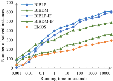
We conduct experiments to validate the efficacy of our proposed techniques. [Jiang and Zheng, 2023] is one of the most recent references, which said in their paper that their algorithm EMOS was the first effective branch-and-bound algorithm for MDSP. Experiments show that our algorithms are much faster than EMOS on standard datasets. For example, EMOS solved 294 tested instances within 5 hours, while our algorithms solved 399 and 302 tested instances, respectively, within one second. We also mark that there is another recent reference [Inza et al., 2024] that gave an implicit enumeration algorithm for MDSP. However, we could not reproduce their result in the experiments and then we could not compare with this algorithm. We will show the details in Sec. 4.
Paper organization The structure of this paper is as follows: Section 2 provides the definitions and notations used throughout the paper. Section 3 details the techniques and framework of our proposed algorithm. Section 4 presents experimental results, comparing our algorithm with the state-ofthe-art exact algorithm for MDSP. Section 5 compares techniques used by our algorithm with existing results.
2 Definitions and Symbols
Let G = (V,E) denote an undirected graph with the set of vertices V and the set of edges E. An edge (u, v) ∈ E is an unordered pair of vertices u and v. u and v are called endpoints of the edge. An edge is called a self-loop if the two endpoints of it are identical. Two edges with the same endpoints are parallel. Without explicitly stated, neither selfloops nor parallel edges exist in the graphs throughout this paper. Two vertices are adjacent if they are connected by an edge. The neighbors of a vertex v, denoted by N(v), is the set of vertices that are adjacent to v. The closed-neighbors of a vertex v, denoted by N[v], is the union of N(v) and v itself, i.e., N[v] = N(v) ∪ {v}. A vertex v (resp., a vertex set U) is dominated by a vertex set D if v ∈ N[D] (resp., U ⊆ N[D]). If a vertex set D dominates all vertices in G, we call D a dominating set of G. The Minimum Dominating Set Problem (MDSP) aims to find a dominating set of the minimum size in a graph. In this paper, we will consider a more general version of MDSP, called the Extended Minimum Dominating Set Problem (EMDSP). In EMDSP, we are given a graph G = (V,E), two disjoint set of vertices S,X ⊆ V , and another set of vertices I ⊆ V . The goal is to find a smallest set D such that all vertices in V \ I are dominated by D, where S ⊆ D ⊆ V \ X. The set of vertices I is not required to be dominated but vertices in it can be selected to dominate other vertices. The set of vertices X is not allowed to be selected to the solution set to dominate other vertices. The set of vertices S should be always in the solution. We use I = (G, S, X, I) to denote an instance of EMDSP. Obviously, the problem degenerates to MDSP when S = X = I = ∅.
A vertex in S, X and I is called selected, excluded and ignored, respectively. Furthermore, we call vertices in V \ (S ∪ X) undetermined and vertices in V \(N[S]∪I) undominated. The set of dominators of an undominated vertex v is defined as D(v) = N[v] \ X, which is the set of undetermined vertices that dominate v. The coverage of an undetermined vertex v is defined as C(v) = N[v] \ (N[S] ∪ I), which is the set of undominated vertices that v dominates. We also extend the functions D(·) and C(·) to a set of vertices. For a set of vertices Y , we use D(Y ) and C(Y ) to denote the union of dominators and coverages of the vertices in Y , respectively.
We note that EMDSP enables the modeling of many other problems as generalizations of the dominating set problem. For example, the Set Cover Problem can be modeled as an EMDSP instance on a bipartite graph with the two sides corresponding to elements and sets, where all sets should be ignored and all elements should be excluded.
3 The AlgorithmFramework
This paper introduces two algorithms for EMDSP, both of which adhere to the classical branch-and-bound framework. Initially, these algorithms apply reduction rules to simplify the instance, thereby finding a partial solution in polynomial time. If no reduction rules are applicable, the problem is decomposed into several smaller sub-problems. The algorithm then traverses the branches of the search tree, each representing a sub-problem. This operation can exponentially increase the running time. To optimize the algorithm, some branches that cannot lead to an optimal solution are pruned. A commonly used pruning technique is the lower-bound method for minimization problems. When evaluating a (sub) problem, the algorithm compares the best possible solution size of it with the size of the incumbent best solution. If it does not contain a better solution than the best one found so far, the branch is discarded.
There are two critical components in the framework. The first is the design of effective reduction rules to reduce the instances as much as possible. The second is the implementation of efficient branching operations with effective methods to compute lower bounds. Both the quality of the lower bound and the computation time must be considered.
We propose three reduction rules, all of which are utilized in our two algorithms. However, the methods to compute lower bounds in our two algorithms differ. The first algorithm, BIBCO, is a pure combinatorial algorithm with a combinatorial method to compute lower bounds. The second algorithm, BIBLP, uses Linear Programming relaxation of EMDSP to compute the lower bound and prune the search tree. Although computing a single LP relaxation may be timeconsuming, the bound is usually tight, and we may only need to branch a small number of times. As a result, we may solve certain instances faster.
Algorithm 1: BIBSearch(I, D∗ )
Input: An EMDSP instance I = (G, S, X, I) and D∗ , the best solution we have found for G. Output: A minimum dominating set D∗ of G such that S ⊆ D∗ ⊆ V -X. 1 I ′ := Reduce(I) 2 if N[S] = V then 3 if |S| < |D∗ | then D∗ := S 4 return D∗ 5 if |D∗ | ≤ LowerBound(I) then 6 return D∗ 7 Select a vertex v by the criteria described in Sec. 3.1 8 foreach u ∈ D(v) in descending order of |C(u)| do 9 Iu := (G, S ∪ {u},X,D∗ , I) 10 D := BIBSearch(Iu,D∗ ) 11 if |D| < |D∗ | then 12 D∗ :=D 13 X :=X ∪ {u} 14 return D∗3.1 The Algorithm
The pseudo-code in Alg. 1 explains the same algorithm framework of our two algorithms. The algorithm takes an instance I = (G, S, X, I) of EMDSP and a feasible solution D∗ as the input, where D∗ = V \ X initially. The algorithm first applies the reduction rules described in Sec. 3.2 to reduce the input instance. We use Reduce(I) on Line 1 in Alg. 1 to denote the reduction operation. After applying reduction rules, the algorithm checks whether the instance is already solved. If so, the algorithm updates the best solution, then returns the best solution to the caller. If the instance is not solved, the algorithm computes a lower bound of the best possible solution size of the input instance. We use LowerBound(I) to denote the function of compute the lower bound of the instance I. Our two algorithms only differ in the function LowerBound(I) in Line 5, i.e., the method for computing the lower bound. We will describe the details of LowerBound(I) in Sec. 3.3. The algorithm returns when the lower bound is no less than the incumbent best solution. Otherwise, the algorithm recursively solves the sub-problems generated by the following branching method.
- Pick the undominated vertex v that minimizes the number of dominators, |D(v)|.
- If there is a tie, pick the vertex that maximizes the sum of the coverage size of its dominators, ∑u∈D(v) |C(u)|.
- If there is still a tie, pick the smallest-indexed vertex.
The algorithm sort the dominators of v, D(v) by descending order of their coverage size, since vertices with the larger coverage size is intuitively more likely to be included by the smallest solution. When there is a tie, break the ties arbitrarily. Then we enumerate the first vertex in the sorted D(v) to be included by the optimal, as shown in Lines 14-16 in Alg. 1.
3.2 Reduction Rules
Now we explain our function Reduce(I), which will consider three rules. Consider an instance I = (G, S,X, I) of EMDSP. The problem is considered solved when either S ∪ X = V , indicating that there are no undetermined vertices, or when N[S] = V , signifying that there are no undominated vertices. Our approach aims to reduce the number of undetermined and undominated vertices by designing rules to expand the sets S,X. We propose three reduction rules to add vertices to S,X, and I, respectively. Although expanding the set I does not directly affect the termination condition, it increases the likelihood of applying other reduction rules, thereby indirectly reducing the problem scale.
- Rule 1 (Single Dominator). Given an instance I = (G, S,X, I) of EMDSP, if an undominated vertex v has only one dominator u, we add u to S.
- Rule 2 (Subset Coverage). For an instance I = (G, S, X, I) of EMDSP, if there exist two distinct undetermined vertices u, v such that the coverage of u is a subset of N[v], i.e., C(u) = N[u] \ (N[S] ∪ I) ⊆ N[v], we add u to X.
Proof. We assert that I admits an optimal solution that excludes u. Suppose every minimum dominating set under I contains u and let D be any one of them. Let Z = V \(N[D\ {u}]∪I) be the vertices that are not dominated after removing u. Since D is a valid dominating set, any vertex in Z is adjacent to u, implying Z ⊆ N[u]. We have Z ∩ N[S] = ∅ since S ⊆ D\{u}. By the definition of Z, we also have Z ∩I = ∅, therefore Z ⊆ N[u]-\(N[S]∪I). By the definition of u and v, we have Z ⊆ N[u] - \(N[S] ∪ I) ⊆ N[v], which implies D′ = (D \ {u}) ∪ {v} is a solution of I. Therefore, there exists a solution D′ of the same size and excludes u.
- Rule 3 (Ignorable Vertices). For an instance I = (G, S,X, I) of EMDSP, if there exist two distinct undominated vertices u, v such that D(u) = N[u] \ X ⊆ N[v], we add v to I.
Proof. We claim that adding v to I does not alter the solution set of I. That is, a vertex set Y such that S ⊆ Y ⊆ V - X dominates V - (N[S] ∪ I) if and only if Y dominates V - (N[S] ∪ I ∪ {v}). Let Y be a vertex set such that S ⊆ Y ⊆ V - X and Y dominates V - (I ∪ {v}). Since u is undominated in I, we have u /∈ I and Y dominates u. Therefore u ∈ V - (I ∪ {v}), which implies there exists y ∈ Y such that y ∈ D(u). By the definition of u and v, we have D(u) ⊆ N[v], therefore y ∈ N[v], and v is also dominated by Y . As a result, Y dominates V - I, and the reverse side is obvious.
Time Complexity We intergrate our reduction rules into an algorithm that exhaustively applies the rules, as depicted in Algorithm 2. The implementation of the single dominator rule for the entire graph requires O(|V | + |E|) time. This is achieved by enumerating each vertex u and examining its neighbors. For the subset coverage rule, we note that C(u) ⊆ N[v] is equivalent to v ∈ N[w] for all w ∈ C(u). We can select a vertex w0 from C(u) and verify if there exists a v ∈ N[w0] that meets the above condition. Let ∆ represent
Input: An EMDSP instance I = (G, S, X, I). Output: A reduced EMDSP instance I ′ . 1 repeat 2 foreach u ∈ V \ (X ∪ S) do 3 if ∃v ∈ N[u] that D(v) = {u} then 4 S := S ∪ {u} 5 foreach u ∈ V \ (X ∪ S) do 6 if ∃v ∈ V that C(u) ⊆ N[v] then 7 X := X ∪ {u} 8 foreach u ∈ V \ (N[S] ∪ I) do 9 foreach v ∈ V that D(u) ⊆ N[v] do 10 I := I ∪ {v}11 until no changes have been made to I in this iteration 12 return I
the maximum vertex degree of G and w0(u) be the vertex chosen from C(u) when attempting to exclude u. The time complexity of this procedure is as follows:
Consequently, the subset coverage rule can be implemented in O((|V | + |E|)∆) time for the entire graph.
We employ a similar method to implement the ignorable vertices rule, as D(u) ⊆ N[v] is also equivalent to v ∈ N[w] for all w ∈ D(u). The only difference is that we need to iterate through every v ∈ N[w0] and check whether v satisfies the above condition, where the previous procedure exits when it finds any vertex v such that C(u) ⊆ N[v]. However, the worst-case time complexity remains the same. Thus, we can implement the ignorable vertices rule in O((|V | + |E|)∆) time for the entire graph.
In each iteration of the loop, we either increase the size of S, X, I, or we exit the loop. Since the maximum sizes of S, X, and I are O(|V |), the total time complexity to exhaustively apply these rules is O(|V ||E|∆) in the worst case, as we either exit the loop due to no changes to the instance or apply the rules after each iteration.
3.3 Lower Bounds
In this section, we present the lower bounds employed in our two algorithms , i.e., explain the function LowerBound(I). The first algorithm, BIBCO, utilizes two lower bounds: the Disjoint Dominators Lower Bound (DDLB) and the Maximum Coverage Size Lower Bound (MCSLB). On the other hand, the second algorithm, BIBLP, solely uses the LPRelaxation based Lower Bound (LPRLB). For the combinatorial algorithm, we return the maximum value among the two bounds it employs.
Lower Bound 1 (Disjoint Dominators Lower Bound). Let I = (G, S,X, I) be an instance of EMDSP. We define a set Y of undominated vertices as disjoint if any two vertices in Y
have disjoint dominators. We denote by L1(I) the maximum size over all disjoint vertex sets. Consequently, any dominating set under I must have a size of at least |S| +L1(I).
Proof. Let Y = {y1, . . . , y|Y |} be a disjoint vertex set. Any dominating set under I must include at least one vertex from D(yi) for each 1 ≤ i ≤ |Y | since they are not dominated by S. Given that D(yi) are pairwise disjoint and any D(yi) is disjoint to S, the minimum dominating set of I must have a size of at least |S| +L1(I).
Calculating the largest disjoint set is equivalent to solving the Maximum Set Packing Problem, which is proven to be NP-Hard and therefore impractical for our algorithm. To enable this lower bound, we use a greedy algorithm that constructs the disjoint set by selecting the undominated vertex with the fewest number of dominators iteratively. Dominators of the selected vertex will be marked, and the algorithm never selects an undominated vertex with marked dominators. This algorithm can be implemented in O(|E| + |V | log |V |) by sorting the vertices in ascending order of the number of dominators, then checking each vertex in order for the presence of an unmarked dominator.
Lower Bound 2 (Maximum Coverage Size Lower Bound). Let I = (G, S,X, I) be an instance of EMDSP and v1, v2, . . . , v|V-X| be the undetermined vertices under I sorted in descending order of their coverage size. We denote by L2(I) the minimum number such that ∑L2(I) i=1 |C(vi)| ≥ |V \(N[S]∪I)|. That is, we need to select at least L2(I) vertices such that the sum of their coverage size is no less than the number of undominated vertices under I. Any dominating set under I must have a size of at least |S| +L2(I).
Proof. The sum of the coverage size of the vertices in any dominating set of I should be at least |V - \(N[S] ∪ I)|. To achieve this goal, one has to select at least L2(I) vertices from V -X, therefore the minimum dominating set of I must have a size of at least |S| +L2(I).
Lower Bound 3 (LP-Relaxation Lower Bound). Let I = (G, S,X, I) be an instance of EMDSP and let L3(I) be the optimal solution of the following linear program P. Any dominating set under I must have a size of at least |S|+⌈L3(I)⌉.
Proof. We claim that the ILP P ′ obtained by replacing (3) with xv ∈ {0, 1} for all v ∈ V - S - X is equivalent to EMDSP instance I = (G, S,X, I). For any undetermined vertex v ∈ V - S -X, the value of xv denotes whether v is included in the solution, and the objective is to minimize the number of selected vertices. Constraint (2) ensures that for any vertex v not dominated by S, at least one vertex in D(v) = N[v] - X is selected into the solution. Since the replacement of (3) tightened the constraint, the correctness of this lower bound is obvious.
4 Experiments
This section presents an evaluation of the effectiveness of the techniques incorporated into our algorithms. We conducted experiments on four datasets that are commonly used in the literature [Potluri and Singh, 2011; Jovanovic et al., 2010; Cai et al., 2020; Jiang and Zheng, 2023; Inza et al., 2024] to assess the performance of our algorithms.
UDG (Unit Disk Graphs) : This dataset comprises 120 random graphs, divided into two families. These families are used to model wireless networks [Potluri and Singh, 2011]. Each family includes graphs of varying scales, with each scale containing 10 unique graphs generated with random seeds ranging from 0 to 9.
T1 : This dataset includes 530 randomly connected graphs of various scales and densities, as generated in [Jovanovic et al., 2010]. The generation parameters for the graphs in T1 include the number of vertices and edges, and a random seed that ranges from 0 to 9.
Network Repository : We selected 8 categories of networks, totaling 120 graphs, from the well-known Network Repository 1 [Rossi and Ahmed, 2015]. This selection allows us to evaluate our techniques on real-world graphs that have close ties to applications.
BD3/BD6 : In [Inza et al., 2024], the authors generated several sets of random graphs with various densities to evaluate their algorithms for MDSP. However, among all graphs mentioned in its experiment section of [Inza et al., 2024], we were only able to find 38 graphs from the link 2 provided by the authors. BD3 and BD6 correspond to graphs No. 1-18 in Table 4 and graphs No. 1-20 in Table 3 of [Inza et al., 2024], respectively.
Settings Our algorithms are implemented in C++ and compiled using gcc version 9.4.0 with the -O3 flag enabled. We use HiGHS [Huangfu and Hall, 2018] as the LP solver in our algorithms. The authors of [Jiang and Zheng, 2023] have made their source code for EMOS, along with the UDG and T1 datasets, publicly available on Github 3 . All experiments were conducted on a server equipped with an Intel Xeon Gold 6226R CPU and 512 GB of memory, running Ubuntu Server 20.04 LTS. Our codes and the experimental results are published here 4 . The time limit for each trial is set to 5 hours, consistent with [Jiang and Zheng, 2023].
Algorithms We test BIBCO and BIBLP, along with the state-of-the-art exact algorithm EMOS for MDSP in [Jiang and Zheng, 2023]. To compare the effectiveness of our reduction rules with the existing rules proposed in [Cai et al., 2020], we replaced the reduction operations in our two algorithms with the three inference rules proposed in [Cai et al., 2020]. We re-implemented these rules faithfully to fit into our algorithm framework. The names of these two variants have the suffix '-IF'. A comparison between our rules and existing rules is also presented in Sec. 5.2.
1 https://networkrepository.com/
2 https://doi.org/10.17632/rr5bkj6dw5.4
3 https://github.com/huajiang-ynu/ijcai23-mds/
4 https://anonymous.4open.science/r/IJCAI24-MDS-0570/
We also note the recently proposed algorithm BDS in [Inza et al., 2024]. However, we did not include it in our experiments due to the difficulties in reproducing their results. Although we were able to compile their code, their program did not halt in two days even on the smallest case in Table 2. For the same test case (where |V | = 600), their reported optimal solution containing 10 vertices. This is contrary to the solution found by our algorithms and EMOS, which consists of only 9 vertices. Please refer to Table 2 for the results produced by our algorithms.
4.1 Results and Analysis
Figure 1 presents the number of instances solved by the algorithms within a specified time frame. Among all graphs included by the experiment, BIBLP and BIBCO solved 399 and 302 instances, respectively, within one second. In contrast, EMOS only managed to solve 294 instances within a fivehour time limit. Table 1 lists the running times of the tested algorithms on T1, UDG, and Network Repository graphs. We have omitted results on graphs with fewer than 100 vertices for T1 and graphs with fewer than 50 vertices for UDG. For the remaining omitted graph categories in the T1 dataset, none of the tested algorithms have solved graphs where the number of vertices is less than the number of edges.
Powered by LPRLB, BIBLP and BIBLP-IF solved the highest number of instances among these three datasets. BIBLP and BIBCO solved 338 and 230 instances in T1 within the time limit, while EMOS solved only 164 instances. In T1, these two algorithms have similar performance, with BIBLP being approximately 1.5 times faster than BIBLP-IF. When comparing the methods to compute lower bounds, BIBCO is significantly slower than BIBLP in relatively sparse graphs of T1. The performance gap between these two algorithms decreases as the density increases, indicating that the gap between the combinatorial lower bounds and the LP-based lower bounds also decreases with increasing graph density.
In UDG, the difference between BIBLP and BIBLP-IF scales to 10 times due to the structural properties of unit disk graphs. This demonstrates the potential of the new Reduction rules proposed in this paper for real-world applications modeled as unit disk graphs. Both BIBLP and BIBCO solved all instances in UDG within the time limit, while EMOS solved only 65 instances. Among the large graphs of UDG, BIBCO is approximately 2500 times faster than EMOS, and BIBLP is about 100 times faster than BIBCO.
| Dataset: T1 | ||||||
|---|---|---|---|---|---|---|
| |V | | |E| | BIBLP | BIBCO | BIBLP-IF | BIBCO-IF | EMOS |
| 150 | 150 | 0.01 | 0.01 | 0.01 | 633.06(2) | 25.03 |
| 150 | 250 | 0.03 | 1.41 | 0.03 | 28.02 | 334.58 |
| 150 | 500 | 8.18 | 2203.54(4) | 10.46 | 1903.10(4) | 2919.74(9) |
| 150 | 750 | 11.17 | 2386.31(5) | 12.37 | 1134.20(2) | 3000.00(10) |
| 150 | 1000 | 23.97 | 2224.23(4) | 25.76 | 665.26(1) | 3000.00(10) |
| 150 | 2000 | 9.89 | 97.62 | 9.16 | 15.92 | 1851.73 |
| 150 | 3000 | 9.11 | 23.66 | 9.00 | 4.18 | 270.71 |
| 200 | 250 | 0.01 | 0.12 | 0.02 | 1840.26(5) | 2900.47(7) |
| 200 | 500 | 307.25(1) | 2927.73(9) | 18.07 | 3000.00(10) | 3000.00(10) |
| 200 | 750 | 166.89 | 3000.00(10) | 200.27 | 3000.00(10) | 3000.00(10) |
| 200 | 1000 | 789.56 | 3000.00(10) | 984.52 | 3000.00(10) | 3000.00(10) |
| 200 | 2000 | 1450.30 | 3000.00(10) | 1559.50 | 3000.00(10) | 3000.00(10) |
| 200 | 3000 | 656.70 | 3000.00(10) | 602.74 | 3000.00(10) | 3000.00(10) |
| 250 | 250 | 0.01 | 0.01 | 0.01 | 3000.00(10) | 3000.00(10) |
| 250 | 500 | 13.83 | 2783.49(9) | 19.06 | 3000.00(10) | 3000.00(10) |
| 250 | 750 | 1030.34(1) | 3000.00(10) | 1054.77(1) | 3000.00(10) | 3000.00(10) |
| 250 | 1000 | 2504.13(7) | 3000.00(10) | 2508.30(7) | 3000.00(10) | 3000.00(10) |
| 300 | 300 | 0.01 | 0.01 | 0.01 | 3000.00(10) | 3000.00(10) |
| 300 | 500 | 5.80 | 2852.50(9) | 5.36 | 3000.00(10) | 3000.00(10) |
| 300 | 750 | 1751.27(3) | 3000.00(10) | 2081.97(6) | 3000.00(10) | 3000.00(10) |
| 800 | 1000 | 23.51 | 3000.00(10) | 32.57 | 3000.00(10) | 3000.00(10) |
| Dataset: UDG | ||||||
| |V | | Type | BIBLP | BIBCO | BIBLP-IF | BIBCO-IF | EMOS |
| 250 | A | 0.01 | 0.01 | 0.08 | 1518.49(4) | 443.42 |
| 250 | B | 0.01 | 0.01 | 0.03 | 54.80 | 9.70 |
| 500 | A | 0.05 | 1.16 | 0.96 | 3000.00(10) | 3000.00(10) |
| 500 | B | 0.02 | 0.08 | 0.07 | 1143.27(3) | 1869.86(5) |
| 800 | A | 0.06 | 0.96 | 0.53 | 3000.00(10) | 3000.00(10) |
| 800 | B | 0.29 | 96.77 | 7.94 | 3000.00(10) | 3000.00(10) |
| 1000 | A | 0.07 | 2.60 | 0.55 | 3000.00(10) | 3000.00(10) |
| 1000 | B | 0.78 | 577.89 | 43.06 | 3000.00(10) | 3000.00(10) |
| Dataset: Network Repository | ||||||
| Class | # BIBLP | BIBCO | BIBLP-IF | BIBCO-IF | EMOS | |
| bio | 30 | 1043.72(3) | 1576.04(5) | 1846.86(6) | 6004.69(20) | 6276.41(20) |
| eco | 6 | 0.01 | 0.01 | 0.01 | 0.01 | 0.01 |
| econ | 15 | 5.48 | 1200.00(4) | 1.98 | 1200.03(4) | 1208.10(4) |
| 6 | 27.58 | 300.00(1) | 300.01(1) | 600.03(2) | 600.01(2) | |
| fb | 9 | 0.01 | 0.01 | 0.01 | 0.01 | 2700.00(9) |
| ia | 20 | 322.88(1) | 600.06(2) | 576.26(1) | 2400.04(8) | 1932.27(6) |
| prox | 13 | 300.01(1) | 300.03(1) | 555.91(1) | 600.00(2) | 300.23(1) |
| soc | 21 | 1865.57(6) | 1804.32(6) | 1532.08(5) | 3308.17(11) | 4162.67(13) |
Although it is hard to approximate MDSP in power-law graphs [Gast et al., 2015], which is a popular model for modeling real-world graphs, BIBLP, BIBCO, BIBLP-IF, BIBCOIF, and EMOS, powered by the reduction rules, solved 92, 92, 89, 68, and 50 real-world instances in 1 second, respectively.
We also tested our algorithms on random graphs that are extremely dense. The graph density, calculated as 2|E|/|V |(|V | - 1) of the BD3 and BD6 datasets is approximately 0.9 and 0.8, respectively. In BD3, BIBCO is about 4 times faster than BIBLP. As observed in the T1 dataset, we conjecture that the pruning effect of LPRLB and MCSLB is very close when the graph is dense. DDLB is ineffective in this case since almost every two vertices have common neighbors on these clique-like graphs.
The latest heuristics [Cai et al., 2020] can also find most optimal solutions for the tested graphs within a reasonable time. However, the main value of exact methods is that, when our algorithm halts after 2 minutes, we know that we get the optimal solutions; while the heuristics do not terminate after reaching the optimal.
| Dataset: BD3 | ||||||
|---|---|---|---|---|---|---|
| Graph | |V | | OPT | BIBLP | BIBCO | BIBLP-IF | BIBCO-IF |
| Grafo111 | 600 | 9 | 1328.20 | 200.65 | 7370.95 | 205.48 |
| Grafo113 | 610 | 9 | 1788.78 | 235.23 | 8134.04 | 515.26 |
| Grafo115 | 620 | 9 | 2870.49 | 740.37 | 9310.53 | 590.75 |
| Grafo117 | 630 | 9 | 1657.88 | 247.16 | 8137.22 | 354.10 |
| Grafo119 | 640 | 9 | 1866.73 | 296.23 | 10777.83 | 498.55 |
| Grafo121 | 650 | 7 | 2815.75 | 525.16 | 3507.69 | 108.38 |
| Grafo123 | 660 | 7 | 2566.70 | 323.90 | 3391.31 | 105.72 |
| Grafo125 | 670 | 7 | 2645.39 | 328.75 | 3838.27 | 111.19 |
| Grafo127 | 680 | 9 | 9927.35 | 4834.13 | 13205.36 | 1008.49 |
| Grafo129 | 690 | 7 | 31423.13 | 17273.19 | 16225.74 | 1565.25 |
| Grafo131 | 700 | 9 | 4868.43 | 1295.20 | 13700.40 | 967.99 |
| Grafo133 | 710 | 7 | 4111.80 | 589.15 | 5074.82 | 145.90 |
| Grafo135 | 720 | N/A | N/A | N/A | N/A | N/A |
| Grafo137 | 730 | 9 | 12201.85 | 5852.46 | fail | 1520.00 |
| Grafo139 | 740 | 9 | 3967.32 | 482.95 | 16573.49 | 716.58 |
| Grafo141 | 750 | N/A | N/A | N/A | N/A | N/A |
| Grafo143 | 760 | N/A | N/A | N/A | N/A | N/A |
| Grafo145 | 770 | 9 | 5301.70 | 695.51 | fail | 1145.64 |
| Dataset: BD6 | ||||||
| Graph | |V | | OPT | BIBLP | BIBCO | BIBLP-IF | BIBCO-IF |
| Grafo457 | 1012 | 5 | 0.59 | 3.88 | 0.48 | 3.00 |
| Grafo458 | 1014 | 5 | 0.73 | 4.08 | 0.41 | 3.27 |
| Grafo460 | 1018 | 5 | 1.49 | 23.16 | 1.49 | 3.65 |
| Grafo462 | 1022 | 5 | 0.77 | 3.93 | 0.45 | 3.17 |
| Grafo464 | 1026 | 5 | 1.25 | 18.74 | 1.44 | 3.59 |
| Grafo466 | 1030 | 5 | 1.48 | 26.36 | 1.16 | 2.89 |
| Grafo469 | 1036 | 5 | 0.72 | 3.55 | 0.41 | 2.54 |
| Grafo471 | 1040 | 5 | 0.82 | 4.45 | 0.55 | 3.57 |
| Grafo472 | 1042 | 5 | 1.50 | 22.70 | 1.14 | 3.21 |
| Grafo474 | 1046 | 5 | 0.65 | 3.43 | 0.36 | 3.24 |
| Grafo480 | 1058 | 5 | 1.31 | 21.69 | 1.05 | 3.89 |
| Grafo483 | 1064 | 5 | 0.86 | 4.01 | 0.49 | 3.27 |
| Grafo484 | 1066 | 5 | 1.48 | 25.27 | 1.29 | 3.30 |
| Grafo485 | 1068 | 4 | 0.43 | 0.30 | 0.26 | 2.52 |
| Grafo488 | 1074 | 5 | 1.27 | 25.67 | 1.53 | 3.17 |
| Grafo491 | 1080 | 5 | 0.86 | 4.35 | 0.62 | 3.24 |
| Grafo492 | 1082 | 5 | 1.53 | 28.93 | 1.82 | 4.36 |
| Grafo494 | 1086 | 5 | 1.47 | 25.02 | 1.50 | 3.30 |
| Grafo499 | 1096 | 5 | 0.96 | 5.41 | 0.58 | 2.99 |
| Grafo500 | 1098 | 5 | 0.82 | 3.91 | 0.50 | 2.84 |
4.2 Evaluating the Lower Bounds
We note that the computational cost of combinatorial bounds is much less than that of LP bounds. For some cases (e.g., the BD3 dataset), a significant computational cost is required to obtain a slightly better (or even the same) bound, which actually reduces the efficiency of the algorithm. Therefore, we need to do some trade-offs, as both bound types have their own scenarios for use.
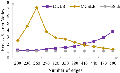
We also conduct experiments to demonstrate the necessity of both combinatorial lower bounds. We generate random graphs with 100 vertices under the Erd˝os-R´enyi model in 11 different densities. For each density we generate 10 different graphs. For the BIBCO algorithm, we disable DDLB and MCSLB seperately and test it on the 110 graphs. As shown in Fig. 2, DDLB is the most effective when the density is relatively low. When the density is high, MCSLB is more effective than DDLB. For middle-sparse graphs, disable any of them enlarges the search space by 1.5-2x.
5 Relation to ExistingWorks
This section discuss the relations of the techniques proposed by this paper with existing results in MDSP.
5.1 Existing Exact Algorithms
Previous strongest theoretical results on exact algorithms for MDSP include two branching algorithms proposed by [Iwata, 2011], one in O(1.4864n ) time and polynomial space, and one O(1.4689n ) time and space. Recently, [Jiang and Zheng, 2023] proposed an exact algorithm EMOS for MDSP based on the branch-and-bound framework and a novel lower bound, which is efficient in practice. The main difference between EMOS and our algorithms is the running context of the branching algorithm, where EMOS does not consider X and I throughout the branching procedure. Based on binary search and heuristic prioritized enumeration of dominating sets, [Inza et al., 2024] designed an exact implicit enumeration algorithm for MDSP. However, as mentioned above, we could not reproduce their result.
5.2 Existing Reduction Rules
In [Alber et al., 2004], two reduction rules for MDSP are proposed in a kernelization algorithm for MDSP in planar graphs. The simpler one are frequently used in the recent literatures [Jiang and Zheng, 2023; Inza et al., 2024]. In [Cai et al., 2020], the authors use a mapping V → {0, 1, undetermined} to represent a partial solution of MDSP. Vertices with value 0 and 1 corresponds to the excluded and selected vertices in the definition of EMDSP. Among the 4 inference rules proposed in their article, 3 are used in their implementation to reduce the problem instance. We note that our Reduction rules extend their 3 implemented rules. The reasons are listed below.
Isolated vertex rule This rule is a special case of our Single Dominator rule when v = u.
Leaf rule Let v be the vertex adjacent to only one vertex u. In this case, we have C(v) = {u, v} ⊆ N(u) and by the Subset Coverage rule we may exclude v from the solution. Subsequently, we have D(v) = N(v) \ X = {u}, and by the Single Dominator rule we must include u into the solution.
- Undominated vertices
- Dominated vertices
- Excluded vertices
- Selected vertices
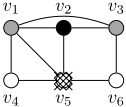
Figure 3: An exemplary EMDSP instance I = (G, S = {v2}, X = {v5}, I = ∅) that demonstrates the superiority of the Disjoint Set Lower Bound. The algorithm is branching on the dominators of v2, and the branch that selects v5 is already explored, and the incumbent solution is {v3, v5}. Since G2 is the complete graph K6, ISLB always yield 1 for any vertex set U ⊆ V . For DDLB, the dominators of v4 and v6 are {v1} and {v3}, respectively. In this case, the output of DDLB is 3 since the dominators of v4 and v6 are disjoint, and v2 is already selected into the solution.
For the case that every vertex in N(v)\u are excluded, this rule needs condition C(v) = {u, v} ⊆ N(u) to hold.
Triangle rule Let {u, v,w} be a triangle in the graph that N[{u, v}] = {u, v,w}. Since C(u) = {u, v,w} \ N[S] ⊆ N[w], we exclude u (and v, for the same reason) from the solution by the Subset Coverage rule. Then we have D(u) = N[u] \ X = {w} and we must select w into the solution by the Single Dominator rule.
5.3 Existing Lower Bounds
Given a graph G. A subgraph of G is a graph G′ = (V ′ , E′ ) such that V ′ ⊆ V and E′ ⊆ E. The subgraph induced by I ⊆ V is the graph obtained by removing all vertices other than I from G and their incident edges, denoted by G[I]. The 2-hop graph of G is the graph obtained by connecting every pair of vertices in G who have at least one common closed neighbor. The 2-hop graph of G is denoted by G2 . In [Jiang and Zheng, 2023], an intricate branching algorithm is designed by the authors with the following lemma:
Lemma 3 [Jiang and Zheng, 2023] Given a graph G = (V,E) and its G2 . Let U be a subset of V and S be an independent set in G2 [U]. For any subset D ⊆ V that can dominate U in G, it holds that |D| ≥ |S|.
This lower bound is designed specifically for MDSP. For an EMDSP instance I = (G, S,X, I), DDLB is equivalent to ISLB when we set U = N[S] \ I and X = ∅. However, on the general case that X ̸= ∅, DDLB is always at least, or even more tighter then ISLB. The reason is that any two vertices that share dominators are 2-hop adjacent, but not vice versa. See Fig. 3 for an example.
6 Conclusion
In this work, we introduce a novel branch-and-bound framework together with three reduction rules and three lower bounds for solving EMDSP. Based on these techniques, we propose two algorithms that shares the reduction rules but differs in the lower bounds they use. One of them is the purely combinatorial algorithm BIBCO, and the other one that uses LP to tighten the bound is named BIBLP. When compared to the state-of-the-art exact algorithm EMOS, both algorithms demonstrates superior empirical speed and solves a significantly larger number of instances within the 5 hour time limit.
Acknowledgements
This work is supported by National Natural Science Foundation of China under grants 62372095 and 62172077, and Natural Science Foundation of Sichuan Province of China under grant 2023NSFSC0059.
@inproceedings{ijcai2024p780,
  title     = {Exactly Solving Minimum Dominating Set and Its Generalization},
  author    = {Xiong, Ziliang and Xiao, Mingyu},
  booktitle = {Proceedings of the Thirty-Third International Joint Conference on
               Artificial Intelligence, {IJCAI-24}},
  publisher = {International Joint Conferences on Artificial Intelligence Organization},
  editor    = {Kate Larson},
  pages     = {7056--7064},
  year      = {2024},
  month     = {8},
  note      = {Main Track},
  doi       = {10.24963/ijcai.2024/780},
  url       = {https://doi.org/10.24963/ijcai.2024/780},
}
TY - CPAPER TI - Exactly Solving Minimum Dominating Set and Its Generalization AU - Xiong, Ziliang AU - Xiao, Mingyu T2 - Proceedings of the Thirty-Third International Joint Conference on Artificial Intelligence, IJCAI-24 PB - International Joint Conferences on Artificial Intelligence Organization PY - 2024 SP - 7056 EP - 7064 DO - 10.24963/ijcai.2024/780 UR - https://doi.org/10.24963/ijcai.2024/780 ER -Copied
Machine-readable versions of this paper, for tools and AI agents:





