
Towards Efficient MCMC Sampling in Bayesian Neural Networks by Exploiting Symmetry (Extended Abstract)
Proceedings of the Thirty-Third International Joint Conference on Artificial Intelligence. Sister Conferences Best Papers. Pages 8466-8470.
https://doi.org/10.24963/ijcai.2024/943
Keywords
- Uncertainty in AI: UAI: Tractable probabilistic models
- Uncertainty in AI: UAI: Inference
- Machine Learning: ML: Bayesian learning
- Machine Learning: ML: Probabilistic machine learning
Abstract
Bayesian inference in deep neural networks is challenging due to the high-dimensional, strongly multi-modal parameter posterior density landscape. Markov chain Monte Carlo approaches asymptotically recover the true posterior but are considered prohibitively expensive for large modern architectures. We argue that the dilemma between exact-but-unaffordable and cheap-but-inexact approaches can be mitigated by exploiting symmetries in the posterior landscape. We show theoretically that the posterior predictive density in Bayesian neural networks can be restricted to a symmetry-free parameter reference set. By further deriving an upper bound on the number of Monte Carlo chains required to capture the functional diversity, we propose a straightforward approach for feasible Bayesian inference.
- [Chen et al., 1993] An Mei Chen, Haw-minn Lu, and Robert Hecht-Nielsen. On the Geometry of Feedforward Neural Network Error Surfaces. Neural Computation, 5(6):910- 927, 1993.
- [Daxberger et al., 2021] Erik Daxberger, Agustinus Kris- tiadi, Alexander Immer, Runa Eschenhagen, Matthias Bauer, and Philipp Hennig. Laplace Redux -Effortless Bayesian Deep Learning. In 35th Conference on Neural Information Processing Systems (NeurIPS 2021), 2021.
- [Dua and Graff, 2017] Dheeru Dua and Casey Graff. UCI machine learning repository, 2017.
- [Gelman et al., 2014] Andrew Gelman, Jessica Hwang, and Aki Vehtari. Understanding predictive information cri- teria for Bayesian models. Statistics and Computing, 24(6):997-1016, 2014.
- [Hecht-Nielsen, 1990] Robert Hecht-Nielsen. On the alge- braic structure of feedforward network weight spaces. In Advanced Neural Computers, pages 129-135. Elsevier, 1990.
- [Hoffman and Gelman, 2014] Matthew D. Hoffman and An- drew Gelman. The No-U-Turn Sampler: Adaptively Set- ting Path Lengths in Hamiltonian Monte Carlo. Journal of Machine Learning Research, 15(47):1593-1623, 2014.
- [Hüllermeier and Waegeman, 2021] Eyke Hüllermeier and Willem Waegeman. Aleatoric and Epistemic Uncertainty in Machine Learning: An Introduction to Concepts and Methods. Machine Learning, 2021.
- [Izmailov et al., 2021] Pavel Izmailov, Sharad Vikram, Matthew D. Hoffman, and Andrew Gordon Wilson. What Are Bayesian Neural Network Posteriors Really Like? In Proceedings of the 38th International Conference on Machine Learning, PMLR 139, 2021.
- [Kůrková and Kainen, 1994] Věra Kůrková and Paul C. Kainen. Functionally Equivalent Feedforward Neural Net- works. Neural Computation, 6(3):543-558, 1994.
- [Lakshminarayanan et al., 2017] Balaji Lakshminarayanan, Alexander Pritzel, and Charles Blundell. Simple and Scal- able Predictive Uncertainty Estimation using Deep Ensem- bles. In Proceedings of the 31st Conference on Neural In- formation Processing Systems (NIPS 2017), 2017.
- [MacKay, 1992] David J. C. MacKay. Bayesian Interpola- tion. Neural Computation, 4:415-447, 1992.
- [Petzka et al., 2020] Henning Petzka, Martin Trimmel, and Cristian Sminchisescu. Notes on the Symmetries of 2- Layer ReLU-Networks. Northern Lights Deep Learning Workshop, 1, 2020.
- [Sommer et al., 2024] Emanuel Sommer, Lisa Wimmer, Theodore Papamarkou, Ludwig Bothmann, Bernd Bischl, and David Rügamer. Connecting the Dots: Is Mode- Connectedness the Key to Feasible Sample-Based Infer- ence in Bayesian Neural Networks? In Proceedings of the 41th International Conference on Machine Learning. PMLR, 2024.
- [Sussmann, 1992] Héctor J. Sussmann. Uniqueness of the weights for minimal feedforward nets with a given input- output map. Neural Networks, 5(4):589-593, 1992.
- [Vlačić and Bölcskei, 2021] Verner Vlačić and Helmut Bölcskei. Affine symmetries and neural network iden- tifiability. Advances in Mathematics, 376:107485, 2021.
References were extracted automatically from the PDF and may contain errors.
Full text extracted automatically from the PDF; figures, tables and equations may differ. The PDF is the version of record.
1 Introduction
Bayesian neural networks (BNNs) are a probabilistic formulation of deep learning models and as such provide uncertainty quantification (UQ) in a principled manner. A key component of Bayesian learning is the parameter posterior density that assigns a posterior probability to each parameter value [H¨ullermeier and Waegeman, 2021]. However, the parameter posterior for BNNs is typically highly multi-modal and rarely available in closed form. The classical Markov chain Monte Carlo (MCMC) approach asymptotically recovers the true posterior but is considered prohibitively expensive for BNNs, as the large number of posterior modes prevents a reasonable mixing of chains [Izmailov et al., 2021]. Popular approximation techniques, such as Laplace approximation (LA) [MacKay, 1992; Daxberger et al., 2021] or deep ensembles
∗This extended abstract is based on a preprint that has not undergone peer review or any post-submission improvements or corrections. The Version of Record of this contribution is published in Machine Learning and Knowledge Discovery in Databases: Research Track. ECML PKDD 2023. Lecture Notes in Computer Science, vol 14169. Springer, and is available online at https: //doi.org/10.1007/978-3-031-43412-9 27.
(DE) [Lakshminarayanan et al., 2017], therefore focus on local regions of the posterior landscape. While these methods are faster than traditional MCMC and perform well in many applications, they systematically omit regions of the parameter space that might be decisive for meaningful UQ [Izmailov et al., 2021].
In this work, we challenge the presumed infeasibility of MCMC for neural networks (NNs) and propose to exploit the-in this context, rarely considered-unidentifiability property of NNs, i.e., the existence of two or more equivalent parameter values that describe the same input-output mapping. We refer to these equivalent values as equioutput parameter states. These emerge from certain activation functions [K˚urkov´a and Kainen, 1994; Chen et al., 1993; Petzka et al., 2020], as well as the free permutability of neuron parameters in hidden layers [Hecht-Nielsen, 1990], and can be transformed into one another.
Our Contributions. We analyze the role of posterior space redundancies in quantifying BNN uncertainty, making the following contributions: 1) Rather than sampling the entire parameter space, we show that the full posterior predictive density (PPD) can be obtained from a substantially smaller reference set containing uniquely identified parameter states in function space. 2) We propose an estimation procedure for the number of Monte Carlo chains required to discover functionally diverse modes, providing a practical guideline for sampling from the parameter space of multi-layer perceptrons (MLPs). 3) We supply experimental evidence that our approach yields superior predictive performance compared to standard MCMC and local approximation methods.
2 Background and Notation
In this work, we consider NNs of the following form. Let f : X → Y represent an MLP with K layers, where layer l ∈ {1, . . . ,K} consists of Ml neurons, mapping a feature vector x = (x1, . . . , xn)⊤ ∈ X ⊆ Rn , n ∈ N, to an outcome vector f(x) =: ˆ y = (ˆ y1, . . . , ˆ ym)⊤ ∈ Y ⊆ Rm, m ∈ N, to estimate y = (y1, . . . , ym)⊤ ∈ Y. The i-th neuron in the l-th layer of the MLP is associated with the weights wlij, j = 1, . . . ,Ml-1, and the bias bli. We summarize all the MLP parameters in the vector θ := (w211, . . . ,wKMKMK-1 , b21, . . . , bKMK )⊤ ∈ Θ ⊆ Rd and write fθ to make clear that the MLP is parameterized by θ. For each hidden layer l ∈ {2, . . . ,K - 1}, the inputs are linearly transformed and then activated by a function a. More specifically, we define the pre-activations of the i-th neuron in the l-th hidden layer as oli = ∑Ml-1 j=1 wlijz(l-1)j + bli with post-activations z(l-1)i = a(o(l-1)i) from the preceding layer. For the input layer, we have z1i = xi, i = 1, . . . , n, and for the output layer, zKi = ˆ yi, i = 1, . . . ,MK.
Predictive Uncertainty. In the Bayesian paradigm, a prior density p(θ) is imposed on the parameters. Using Bayes' rule, the parameter posterior density p(θ|D) = p(D|θ)p(θ)/p(D) updates this prior belief based on the information encoded in the likelihood p(D|θ), given a dataset D = {(x(1) , y(1) ), . . . , (x(N) , y(N) )}. The PPD p(y∗ |x∗ ,D) quantifies the predictive or functional uncertainty of the model for a new observation (x∗ , y∗ ) ∈ X × Y. Since p(y∗ |x∗ ,D) = ∫Θ p(y∗ |x∗ , θ)p(θ|D) dθ, deriving this uncertainty requires access to the posterior density p(θ|D), which can be estimated from MCMC sampling.
2.1 Equioutput Transformations
Let us now characterize the notion of equioutput parameter states, and the transformations to convert between them, more formally. Two parameter states θ, θ′ are considered equioutput if the maps fθ, fθ′ yield the same outputs for all possible inputs from X . We denote this equivalence relation by ∼:
The equioutput relation is always defined with respect to a particular MLP f. All MLPs with more than one neuron in at least one hidden layer exhibit such equioutput parameter states that arise from permutation invariances of the inputoutput mapping [Hecht-Nielsen, 1990; K˚urkov´a and Kainen, 1994]. Since the operations in the pre-activation of the i-th neuron in the l-th layer commute, the Ml > 1 neurons of a hidden layer l can be freely interchanged by permuting their associated parameters. In addition, equioutput transformations can arise from the use of certain activation functions with inherent symmetry properties. For example, in the case of tanh, the signs of corresponding parameters can be flipped using tanh(x) = -tanh(-x). We consider transformation maps that are linear in θ and induce a finite amount of equioutput transformation matrices, which includes, for example, the tanh activation function. More specifically, let FT : Θ → Θ, θ ↦→ Tθ, T ∈ Rd×d , be an activationrelated transformation of a parameter vector that might, for instance, encode an output-preserving sign flip. FT constitutes an equioutput transformation if fθ(·) = fFT (θ)(·). We collect all output-preserving transformation matrices T in the
Similarly, let FP : Θ → Θ, θ ↦→ Pθ, P ∈ {0, 1}d×d , be a transformation that permutes elements in the parameter vector. We define the set of permutation matrices that yield equioutput parameter states as
The cardinality of P is at least ∏K-1 l=2 Ml! [Hecht-Nielsen, 1990] when traversing through the NN from the first layer in a sequential manner, applying to each layer permutations that compensate for permutations in its predecessor. Since activation functions operate neuron-wise, activation- and permutation-related equioutput transformations do not interact (for instance, we could permute the associated weights of two neurons and later flip their sign). We can, therefore, define arbitrary combinations of activation and permutation transformations as E = {E = TP ∈ Rd×d , T ∈ T , P ∈ P | fθ(·) = fFE(θ)(·)}. The transformation matrices in E will exhibit a blockdiagonal structure with blocks corresponding to network layers. This is due to the permutations P affecting both incoming and outgoing weights, but only in the sense that two incoming and two outgoing weights swap places, never changing layers. The activation-related sign flips or rescalings occur neuron-wise, making T a diagonal matrix that does not alter the block-diagonal structure of P .
For the cardinality of the set E of equioutput transformations, we can establish a lower bound that builds upon the minimum cardinality of P: |E| ≥ ∏K-1 l=2 Ml! · |Tl|, where |Tl| denotes the number of activation-related transformations applicable to neurons in layer l. From this, it becomes immediately clear that the amount of functional redundancy increases rapidly with the network size (see also Figure 1).
3 Efficient Sampling
3.1 Posterior Reference Set
As introduced in Section 2, for each parameter state θ of an NN, there are functionally redundant counterparts θ′ related to θ by an equioutput transformation, such that fθ(·) = fθ′ (·). We can use this equivalence relation to dissect the parameter space Θ into disjoint equivalence classes. For this, let the reference set S1 be a minimal set of representatives of each equivalence class (cf. open minimal sufficient search sets in [Chen et al., 1993]). All parameter states in S1 are functionally diverse, i.e., θ, ˜ θ ∈ S1 ⇒ θ ̸∼ ˜ θ, and each element in Θ is equivalent to exactly one element in S1. For a finite amount of equioutput transformations, as in the case of tanh-activated MLPs (finite possibilities of sign-flip combinations of hidden neurons), the NN parameter space can then be dissected into |E| disjoint representative sets, which contain equioutput transformations of the elements of the reference set, in the following way.
Proposition 1 (Parameter space dissection). Let S1 be the reference set of uniquely identified network parameter states. Then, for a finite number of equioutput transformations, it holds that the parameter space can be dissected into |E| disjoint, non-empty representative sets up to a set S 0 ⊂ Θ, i.e.,
where Sj ∼= {θ | θ = Ejθ′ ∀θ′ ∈ S1,Ej ∈ E} and ˙∪ denotes the union over disjoint sets. We use S 0 as a residual quantity to account for cases that cannot be assigned unambiguously to one of the sets Sj because they remain unchanged even under a transformation with non-identity matrices Ej ∈ E.
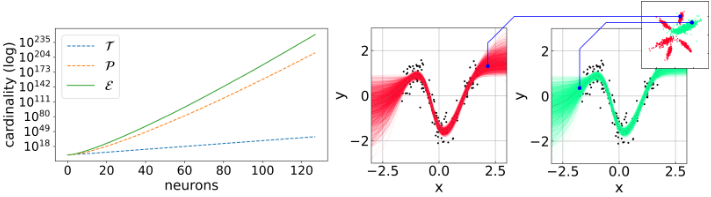
The edge cases that make up S 0 exist, for instance, on the boundary of two classes [Chen et al., 1993] or in degenerated cases [Sussmann, 1992; Vlaˇci´c and B¨olcskei, 2021].
Equioutput parameter states have the same posterior probabilities p(θ|D) = p(Eθ|D) if the prior is transformationinvariant. Moreover, equioutput parameter states produce by definition the same predictions p(y∗ |x∗ , θ) = p(y∗ |x∗ , Eθ) for any E ∈ E. Thus, the following corollary holds.
Corollary 1 (Reformulated posterior predictive density). Let E be finite. As in Proposition 1, consider the disjoint nonempty sets Sj, j ∈ {1, . . . , |E|}, and residual space S 0 . If the prior density p(θ) is transformation-invariant, then the posterior predictive density expresses as
Corollary 1 follows from Proposition 1 and the assumption of transformation-invariant prior densities, which is often satisfied in practice (e.g., for widely-applied isotropic Gaussian priors). We can further approximate (2) by (3) as the set S 0 ⊂ Rd is of negligible size (depending on Θ, potentially even with zero Lebesgue measure).
As a consequence of Corollary 1, the PPD can be obtained up to the residual set by only integrating over uniquely identified parameter states from one of the sets Sj, with a multiplicative factor |E| that corrects the probability values by the amount of redundancy in the posterior. In other words, only a fraction 1/|E| of the posterior must be sampled in order to infer a set of uniquely identified parameter states of the NN, and thus, to obtain the full PPD. This reduces the target sampling space drastically, as illustrated in Figure 1. For example, it allows the posterior space of a single-layer, tanhactivated network with 128 neurons to be effectively reduced to a 10254 -th of its original size.
How to Obtain a Representative Set? When using Monte Carlo to approximate Equation (3), it is not necessary to actually constrain the sampling procedure to a specific set Sj. Since any equioutput transformation is known a priori, we just need to be aware of the fact that each sample can theoretically be mapped to different representative sets after running the sampling procedure. Hence, for the calculation of the PPD integral, the samples can remain scattered across the various representative sets as long as they cover all functionally diverse parameter states.
3.2 An Upper Bound for Markov Chains
The question remains how many samples are needed to approximate a set of uniquely identified parameter states sufficiently well. Even in a symmetry-free setting, BNN posteriors can exhibit multiple functionally diverse modes representing structurally different hypotheses, depending on the network architecture and the underlying data-generating process. In the following, we assume ν ∈ N functionally diverse modes with the goal of visiting every mode or its local proximity at least once when running MCMC. As the ability to switch from one mode to another within a chain depends on various factors, such as the acceptance probability and the current state of other parameters, increasing the number of samples per chain does not necessarily correlate with the number of visited modes. We, therefore, propose to focus on the number of independent chains, rather than the number of samples per chain, to effectively control the number of visited modes. This further allows us to derive an upper bound for the number of independent chains that are required to visit every mode at least once. The number of samples from each chain will then ultimately determine the approximation quality. In practice, given a user-defined number of maximal resources ρ (e.g., CPU cores), the following proposition provides a lower bound on the probability that the number of chains G necessary to visit every mode remains below the resource limit of the user (i.e., G < ρ).
Proposition 2 (Probabilistic bound for sufficient number of Markov chains). Let π1, . . . , πν be the respective probabilities of the ν functionally diverse modes to be visited by an independently started Markov chain and ΠJ := ∑j∈J πj. Then, given ρ chains and ι(ν, q) = (-1)ν-1-q ,
| MCMC (ours) | MCMC (s.c.) | DE | |
|---|---|---|---|
| DS | -0.59 (± 0.12) | -0.59 (± 0.12) | -2.13 (± 0.03) |
| DI | 0.91 (± 0.09) | 0.91 (± 0.09) | -2.02 (± 0.02) |
| DR | 0.95 (± 0.08) | 0.95 (± 0.08) | -2.20 (± 0.02) |
| Airfoil | 0.92 (± 0.05) | 0.72 (± 0.10) | -2.17 (± 0.01) |
| Concrete | 0.26 (± 0.07) | 0.25 (± 0.07) | -2.03 (± 0.01) |
| Diabetes | -1.18 (± 0.08) | -1.22 (± 0.09) | -2.09 (± 0.04) |
| Energy | 2.07 (± 0.46) | 2.38 (± 0.11) | -1.99 (± 0.02) |
| ForestF | -1.43 (± 0.45) | -1.69 (± 0.49) | -2.20 (± 0.02) |
| Yacht | 3.31 (± 0.21) | 0.15 (± 0.09) | -2.18 (± 0.03) |
Note that this bound is independent of the NN architecture and only depends on the assumptions about the number and probabilities of functionally diverse modes ν, disregarding symmetric copies. Proposition 2 can be used to calculate the number of MCMC chains given certain assumptions-for example, from domain knowledge, or in a worst-case scenario calculation-and thus provides practical guidance for MCMC sampling of MLPs. Judging by the comparably high predictive performance of local approximations such as LA and DE [MacKay, 1992; Lakshminarayanan et al., 2017], we conclude that a small amount of functional modes is reasonable to assume in practice. Our qualitative experiments in Section 4 support this supposition.
4 Experiments
In all experiments, we employ a Bayesian regression model with a normal likelihood function, standard normal prior for parameters θ, and a truncated standard normal prior restricted to the positive real line for the variance of the normal likelihood, which we treat as a nuisance parameter. Depending on the task, we either use a No-U-Turn sampler [Hoffman and Gelman, 2014] with 210 warmup steps to collect a single sample from the posterior or derive the maximum-a-posteriori estimator using a gradient-based method.
Performance Comparison. In our first experiment, we demonstrate the predictive performance of BNNs, where the PPD is calculated based on MCMC sampling, using the derived upper bound for the number of chains (ours). In this case, we collect one sample per chain for G chains, and thus G samples in total. This is compared to MCMC sampling collecting G samples from a single chain (s.c.), and DE with ten ensemble members on three synthetic datasets (DS, DI , and DR) as well as benchmark data from UCI [Dua and Graff, 2017]. We use a NN with three hidden layers of 16 neurons each and tanh activations. Furthermore, we assume three functionally diverse modes ν = 3 and mode probabilities π1 = 0.57, π2 = 0.35, π3 = 0.08, which leads to an upper bound of G = 1, 274 chains according to (4). To demonstrate the performance of our MCMC-based PPD approximation, we measure the goodness-of-fit on the test data using the log point-wise predictive density (LPPD) [Gelman et al., 2014] with LPPD = log ∫Θ p(y∗ |x∗ , θ)p(θ|D) dθ ≈ log ( 1G ∑Gg=1 p(y∗ |x∗ , θ(g) )), where θ(1) , . . . , θ(G) are G samples obtained across all chains via MCMC sampling from the parameter posterior density p(θ|D). The approximation is evaluated at each test point (x∗ , y∗ ). Table 1 reports the mean LPPD across N ∗ independent test points for each combination of dataset and sampling scheme. Our results clearly indicate that using only a moderate amount of Markov chains yields equal or even better performance than single-chain MCMC and DE in all but one experiment.
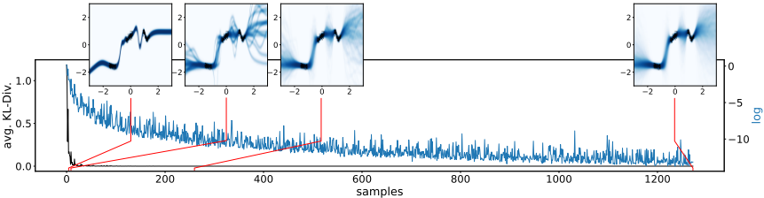
Practical Evaluation of Corollary 1. We further investigate the property derived in Corollary 1 using our proposed upper bound of chains with the same assumptions about mode probabilities as in the previous paragraph. To this end, we analyze the PPD for dataset DI. For every newly collected sample in the MCMC run, the updated PPD is computed approximately on a two-dimensional (input/output) grid. Then, the Kullback-Leibler (KL) divergence between consecutive densities is averaged over the grid of input values of the NN. Despite the high amount of equioutput parameter states |E| ≈ 2.58 · 1054 , the PPD converges after notably fewer than |E| samples (Fig. 2), and plots of the function space indicate the saturation of functional diversity after 1,274 samples.
5 Conclusion
We showed that the PPD for Bayesian MLPs can be obtained from just a fraction of the parameter space, due to the existence of equioutput parameter states, and proposed an upper bound on the number of MCMC chains to guarantee the recovery of every functionally diverse mode. We refer the interested reader to [Sommer et al., 2024] for follow-up work.
Acknowledgements
LW is supported by the DAAD programme Konrad Zuse Schools of Excellence in Artificial Intelligence, sponsored by the German Federal Ministry of Education and Research.
Contribution Statement
JGW and LW contributed equally to this work.
@inproceedings{ijcai2024p943,
  title     = {Towards Efficient MCMC Sampling in Bayesian Neural Networks by Exploiting Symmetry (Extended Abstract)},
  author    = {Wiese, Jonas Gregor and Wimmer, Lisa and Papamarkou, Theodore and Bischl, Bernd and Guennemann, Stephan and Ruegamer, David},
  booktitle = {Proceedings of the Thirty-Third International Joint Conference on
               Artificial Intelligence, {IJCAI-24}},
  publisher = {International Joint Conferences on Artificial Intelligence Organization},
  editor    = {Kate Larson},
  pages     = {8466--8470},
  year      = {2024},
  month     = {8},
  note      = {Sister Conferences Best Papers},
  doi       = {10.24963/ijcai.2024/943},
  url       = {https://doi.org/10.24963/ijcai.2024/943},
}
TY - CPAPER TI - Towards Efficient MCMC Sampling in Bayesian Neural Networks by Exploiting Symmetry (Extended Abstract) AU - Wiese, Jonas Gregor AU - Wimmer, Lisa AU - Papamarkou, Theodore AU - Bischl, Bernd AU - Guennemann, Stephan AU - Ruegamer, David T2 - Proceedings of the Thirty-Third International Joint Conference on Artificial Intelligence, IJCAI-24 PB - International Joint Conferences on Artificial Intelligence Organization PY - 2024 SP - 8466 EP - 8470 DO - 10.24963/ijcai.2024/943 UR - https://doi.org/10.24963/ijcai.2024/943 ER -Copied
Machine-readable versions of this paper, for tools and AI agents:





