
Rethinking Correlation Learning via Label Prior for Open Set Domain Adaptation
Proceedings of the Thirty-Third International Joint Conference on Artificial Intelligence. Main Track. Pages 884-892.
https://doi.org/10.24963/ijcai.2024/98
Keywords
- Computer Vision: CV: Transfer, low-shot, semi- and un- supervised learning
- Computer Vision: CV: Machine learning for vision
Abstract
Open Set Domain Adaptation (OSDA) aims to transfer knowledge from a labeled source domain to an unlabeled target domain, where known classes exist across domains while unknown classes are present only in the target domain. Existing methods rely on the clustering structure to identify the unknown classes, which empirically induces a large identification error if the unknown classes are a mixture of multiple components. To break through this barrier, we formulate OSDA from the view of correlation and propose a correlation metric-based framework called Balanced Correlation Learning (BCL). BCL employs Hilbert-Schmidt Independence Criterion (HSIC) to characterize the separation between unknown and known classes, where HSIC is reformulated as the nodes’ relation on graph. By considering the label prior as variable, theoretical results are derived to analytically show a sufficient condition for desired learning direction for OSDA. Methodologically, the class-balanced HSIC is proposed to preserve domain-invariant and class-discriminative features. With the guarantee of correlation learning, the entropy-based principle can effectively identify the unknown classes via uncertainty. Empirically, extensive evaluations are conducted, where BCL achieves significant performance improvements.
- [Bucci et al., 2020] Silvia Bucci, Mohammad Reza Logh- mani, and Tatiana Tommasi. On the effectiveness of image rotation for open set domain adaptation. In European Con- ference on Computer Vision, pages 422-438, 2020.
- [Fang et al., 2020] Zhen Fang, Jie Lu, Feng Liu, Junyu Xuan, and Guangquan Zhang. Open set domain adapta- tion: Theoretical bound and algorithm. IEEE Transactions on Neural Networks and Learning Systems, 32(10):4309- 4322, 2020.
- [Fukumizu et al., 2007] Kenji Fukumizu, Arthur Gretton, Xiaohai Sun, and Bernhard Schölkopf. Kernel measures of conditional dependence. Advances in Neural Informa- tion Processing Systems, 20, 2007.
- [Ganin and Lempitsky, 2015] Yaroslav Ganin and Victor Lempitsky. Unsupervised domain adaptation by backprop- agation. In International conference on machine learning, pages 1180-1189, 2015.
- [Gretton et al., 2005] Arthur Gretton, Olivier Bousquet, Alex Smola, and Bernhard Schölkopf. Measuring statis- tical dependence with hilbert-schmidt norms. In Interna- tional Conference on Algorithmic Learning Theory, pages 63-77, 2005.
- [He and Niyogi, 2003] Xiaofei He and Partha Niyogi. Lo- cality preserving projections. Advances in Neural Infor- mation Processing Systems, 16, 2003.
- [Jang et al., 2022] JoonHo Jang, Byeonghu Na, Dong Hyeok Shin, Mingi Ji, Kyungwoo Song, and Il-Chul Moon. Unknown-aware domain adversarial learning for open-set domain adaptation. Advances in Neural Information Pro- cessing Systems, 35:16755-16767, 2022.
- [Jing et al., 2021] Mengmeng Jing, Jingjing Li, Lei Zhu, Zhengming Ding, Ke Lu, and Yang Yang. Balanced open set domain adaptation via centroid alignment. In Pro- ceedings of the AAAI Conference on Artificial Intelligence, pages 8013-8020, 2021.
- [Kundu et al., 2020] Jogendra Nath Kundu, Naveen Venkat, Ambareesh Revanur, R Venkatesh Babu, et al. Towards in- heritable models for open-set domain adaptation. In Pro- ceedings of the IEEE/CVF Conference on Computer Vision and Pattern Recognition, pages 12376-12385, 2020.
- [Li et al., 2023] Wuyang Li, Jie Liu, Bo Han, and Yixuan Yuan. Adjustment and alignment for unbiased open set do- main adaptation. In Proceedings of the IEEE/CVF Confer- ence on Computer Vision and Pattern Recognition, pages 24110-24119, 2023.
- [Liu et al., 2019] Hong Liu, Zhangjie Cao, Mingsheng Long, Jianmin Wang, and Qiang Yang. Separate to adapt: Open set domain adaptation via progressive separation. In Proceedings of the IEEE/CVF Conference on computer vi- sion and Pattern Recognition, pages 2927-2936, 2019.
- [Liu et al., 2023] Jieyan Liu, Hongcai He, Mingzhu Liu, Jingjing Li, and Ke Lu. Manifold regularized joint trans- fer for open set domain adaptation. IEEE Transactions on Multimedia, 2023.
- [Long et al., 2013] Mingsheng Long, Jianmin Wang, Guiguang Ding, Jiaguang Sun, and Philip S Yu. Transfer feature learning with joint distribution adaptation. In Proceedings of the IEEE International Conference on Computer Vision, pages 2200-2207, 2013.
- [Luo et al., 2020] Yadan Luo, Zijian Wang, Zi Huang, and Mahsa Baktashmotlagh. Progressive graph learning for open-set domain adaptation. In International Conference on Machine Learning, pages 6468-6478, 2020.
- [Ma et al., 2020] Wan-Duo Kurt Ma, JP Lewis, and W Bas- tiaan Kleijn. The hsic bottleneck: Deep learning without back-propagation. In Proceedings of the AAAI conference on artificial intelligence, pages 5085-5092, 2020.
- [Pan et al., 2020] Yingwei Pan, Ting Yao, Yehao Li, Chong- Wah Ngo, and Tao Mei. Exploring category-agnostic clus- ters for open-set domain adaptation. In Proceedings of the IEEE/CVF Conference on Computer Vision and Pat- tern Recognition, pages 13867-13875, 2020.
- [Panareda Busto and Gall, 2017] Pau Panareda Busto and Juergen Gall. Open set domain adaptation. In Proceed- ings of the IEEE International Conference on Computer Vision, pages 754-763, 2017.
- [Peng et al., 2017] Xingchao Peng, Ben Usman, Neela Kaushik, Judy Hoffman, Dequan Wang, and Kate Saenko. Visda: The visual domain adaptation challenge. arXiv preprint arXiv:1710.06924, 2017.
- [Qu et al., 2023] Sanqing Qu, Tianpei Zou, Florian Röhrbein, Cewu Lu, Guang Chen, Dacheng Tao, and Changjun Jiang. Upcycling models under domain and category shift. In Proceedings of the IEEE/CVF Conference on Computer Vision and Pattern Recognition, pages 20019-20028, 2023.
- [Saenko et al., 2010] Kate Saenko, Brian Kulis, Mario Fritz, and Trevor Darrell. Adapting visual category models to new domains. In Computer Vision-ECCV 2010: 11th Eu- ropean Conference on Computer Vision, Heraklion, Crete, Greece, September 5-11, 2010, Proceedings, Part IV 11, pages 213-226, 2010.
- [Saito et al., 2018] Kuniaki Saito, Shohei Yamamoto, Yoshi- taka Ushiku, and Tatsuya Harada. Open set domain adap- tation by backpropagation. In Proceedings of the Eu- ropean Conference on Computer Vision, pages 153-168, 2018.
- [Saito et al., 2020] Kuniaki Saito, Donghyun Kim, Stan Sclaroff, and Kate Saenko. Universal domain adaptation through self supervision. Advances in Neural Information Processing Systems, 33:16282-16292, 2020.
- [Scheirer et al., 2012] Walter J Scheirer, Anderson de Rezende Rocha, Archana Sapkota, and Terrance E Boult. Toward open set recognition. IEEE Transac- tions on Pattern Analysis and Machine Intelligence, 35(7):1757-1772, 2012.
- [Seidenfeld, 1987] Teddy Seidenfeld. Entropy and uncer- tainty. Foundations of statistical inference, pages 259- 287, 1987.
- [Shermin et al., 2020] Tasfia Shermin, Guojun Lu, Shyh Wei Teng, Manzur Murshed, and Ferdous Sohel. Adversar- ial network with multiple classifiers for open set domain adaptation. IEEE Transactions on Multimedia, 23:2732- 2744, 2020.
- [Tishby et al., 2000] Naftali Tishby, Fernando C Pereira, and William Bialek. The information bottleneck method. arXiv preprint physics/0004057, 2000.
- [Venkateswara et al., 2017] Hemanth Venkateswara, Jose Eusebio, Shayok Chakraborty, and Sethuraman Pan- chanathan. Deep hashing network for unsupervised do- main adaptation. In Proceedings of the IEEE Conference on Computer Vision and Pattern Recognition, pages 5018- 5027, 2017.
- [Wang et al., 2021a] Qian Wang, Fanlin Meng, and Toby P Breckon. Progressively select and reject pseudo-labelled samples for open-set domain adaptation. arXiv preprint arXiv:2110.12635, 2021.
- [Wang et al., 2021b] Wei Wang, Haojie Li, Zhengming Ding, Feiping Nie, Junyang Chen, Xiao Dong, and Zhi- hui Wang. Rethinking maximum mean discrepancy for visual domain adaptation. IEEE Transactions on Neural Networks and Learning Systems, 2021.
- [Xu et al., 2019] Ruijia Xu, Guanbin Li, Jihan Yang, and Liang Lin. Larger norm more transferable: An adaptive feature norm approach for unsupervised domain adapta- tion. In Proceedings of the IEEE/CVF International Con- ference on Computer Vision, pages 1426-1435, 2019.
- [Yan et al., 2017] Ke Yan, Lu Kou, and David Zhang. Learn- ing domain-invariant subspace using domain features and independence maximization. IEEE Transactions on Cy- bernetics, 48(1):288-299, 2017.
- [Zhai Yi-Ming et al., 2023] Ren Chuan-Xian Zhai Yi-Ming, Luo You-Wei, and Dai Dao-Qing. Maximizing conditional independence for unsupervised domain adaptation. SCI- ENCE CHINA Information Sciences, 2023.
- [Zhong et al., 2021] Li Zhong, Zhen Fang, Feng Liu, Bo Yuan, Guangquan Zhang, and Jie Lu. Bridging the the- oretical bound and deep algorithms for open set domain adaptation. IEEE Transactions on Neural Networks and Learning Systems, 2021.
References were extracted automatically from the PDF and may contain errors.
Full text extracted automatically from the PDF; figures, tables and equations may differ. The PDF is the version of record.
1 Introduction
With large amounts of labeled data, deep neural networks have made quite impressive progress on a variety of tasks. However, when the trained network is deployed on a new unlabeled dataset, the original network does not work as well on the new dataset even though the new dataset has the same set of labels as the training set. In general, deep neural networks have poor generalization performance over unseen new domains. To address this problem, a lot of work has been done in the field of Unsupervised Domain Adaptation (UDA) [Long et al., 2013; Ganin and Lempitsky, 2015], which can transfer knowledge from a labeled source domain to an unlabeled target domain. However, existing UDA methods follow a strong assumption that both domains share the same class space, which makes it impossible to make correct predictions about new class samples. In real-world scenarios, in addition to sharing the same classes as the source domain, the target domain also has its own unique classes, which is quite common in object detection [Scheirer et al., 2012].
∗Corresponding Author
In order to solve the above problems, Open Set Domain Adaptation (OSDA) [Panareda Busto and Gall, 2017] has been studied, which can identify novel classes in the target domain as unknown. Recently, several OSDA approaches have been proposed to identify unknown class in the target domain while align known classes shared by both domains. Existing OSDA methods can be divided into two main categories: methods based on adversarial learning; and methods based on subspace learning. For instance, Saito et al. [2018] designed a threshold-based adversarial learning module to recognize unknown class. Based on this idea, some pioneering works [Liu et al., 2019; Jang et al., 2022; Pan et al., 2020] are proposed from the adversarial learning perspective by setting up one or more discriminators to identify unknown class. Wang et al. [2021a] used the pseudo labels of the target domain data to design the adjacency matrix, which is substituted into the LPP [He and Niyogi, 2003] to implement OSDA from the graph embedding perspective. Similarly, some works [Kundu et al., 2020; Jing et al., 2021; Liu et al., 2023] identify unknown class by learning more discriminative subspace that can be used to identify unknown class with the help of the clustering structure of the class.
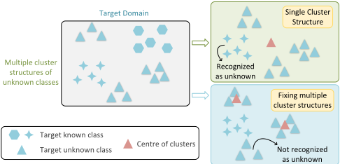
While the above OSDA methods achieve great success, they all have some shortcomings (as shown in Fig. 1). Adversarial learning based methods rely on manually setting threshold when identifying unknown classes. And essentially adversarial learning methods identify unknown classes by the probability vectors output by the discriminator, but the modelling ignores the correlation between the feature and probability vector, so this type of method lacks a reliable basis for directly using probability vectors to identify unknown classes. In addition, methods based on subspace learning identify the unknown classes from the clustering structure of the data, which leads to the fact that when the unknown classes have more than one clustering structure, this kind of methods cannot capture the data structure of the unknown classes well. And even if these methods can focus on multiple cluster structures of unknown classes, the setting of the number of cluster structures needs to be manually adjusted. To address these issues, we complete the identification of unknown classes in terms of correlation. With the help of correlation between features and labels, samples with weak correlation with labels are identified as unknown classes.
In order to realize the identification of unknown classes and the alignment of known classes from the perspective of correlation, we design a framework based on Hilbert-Schmidt Independence Criterion (HSIC), which is an operator norm that evaluates the correlation of variables. In this paper, we propose a theoretically grounded framework, Balanced Correlation Learning (BCL) for OSDA, which contain correlation metrics module to extract discriminative features and align both domains, and entropy measure module to separate known and unknown class. In the correlation metric module, the HSIC is reformulated as the nodes' relation on graph. From the derived theory, by considering the label prior as variable, a sufficient condition for desired learning direction for OSDA have been derived. On the basis of the correlation metric, in order to align the known classes in both domains, we design a class-slicing based HSIC module from the perspective of conditional independence, which can uniformly mix both domains data of each class within the HSIC framework so that the decision boundaries of the source domain are applicable to the target domain data. The above module establishes the correlation between features and labels on both domains, and using this correlation we identify the unknown classes by the probability vector corresponding to the feature. The contributions can be summarized as follows.
- Theoretically, HSIC is reformulated as the nodes' relation on graph, which provides insights into characterizing the learning direction via the adjacency weight. Further, to ensure the desired learning direction for OSDA, a sufficient condition is analytically derived by taking label prior as variable.
- A theory-guided method is proposed for OSDA. It achieves class-balanced HSIC by the designed reweighting technique, where domain-invariant and classdiscriminative features are learned simultaneously. Besides, the reweighting-based method preserves the statis-
- tical property of BCL, i.e., correlation metric property.
- A class slicing variants of HSIC is proposed to achieve correlation learning at the class-conditioned level, which permits the mixture structure of known and unknown classes to be correctly preserved.
- Extensive experiments are conducted, where the results show that the theoretical results are empirically valid and BCL achieve significant improvements over SOTA methods on standard OSDA benchmarks.
2 RelatedWorks
OSDA needs to identify novel classes in target domain as unknown based on the identification of shared known class. Saito et al. [2018] first proposed deep learning algorithm for OSDA. Some work [Fang et al., 2020; Zhong et al., 2021] analyzed OSDA from theoretical perspective and optimized the model from the perspective of error upper bounds. Recent advances mainly focus on two streams of the research, i.e., adversarial learning [Liu et al., 2019; Shermin et al., 2020; Jang et al., 2022] and subspace learning [Wang et al., 2021a; Jing et al., 2021; Liu et al., 2023]. Similar to [Saito et al., 2018], Liu et al. [2019] use multiple binary discriminators to recognize unknown classes, while Jang et al. [2022] transform the domain discriminator into a three-channel discriminator, where one channel is used to recognize unknown class. Jing et al. [2021] recognize unknown class by using class centroid on hyperspheres and Liu et al. [2023] learn more discriminative subspace by adding multiple constraints to the subspace. Adversarial learning-based methods rely on probability vectors to identify unknown classes, but lack the analysis of correlations between feature and label, while subspace learning-based methods do not capture multiple cluster structures of unknown classes well. To model OSDA from correlation, we utilize HSIC [Gretton et al., 2005] as correlation indicator. HSIC can be used to assess the correlation between variables projected onto the reproducing kernel Hilbert spaces. Its empirical estimate is simpler than any other kernel dependence test, so we consider using HSIC to design our framework based on correlation metric. In the field of domain adaptation, there is some work on domain alignment modelling using HSIC [Yan et al., 2017; Ma et al., 2020; Zhai Yi-Ming et al., 2023]. These method demonstrate the efficacy of HSIC in aligning both domains, and HSIC can also be effective in assessing correlation between variables.
3 Method
In this section, we revisit HSIC from the perspective of graph embedding. Combining the obtained theory with the class property of the OSDA problem itself, class-balanced HSIC is used to solve the OSDA problem. On this basis, in order to better align the source and target domains, conditional HSIC based on class slicing achieves conditional independence between features and domains. When the feature and label have a strong correlation, we use entropy to identify the unknown classes from an information theory perspective.
Notations. Let the source and target domains be Xs = {(xsi , ys i )}ns i=1 and Xt = {(xti , yt i )}nt i=1 , which are sampled from distributions P sXY and P tXY , respectively; yt i is not available during training. With the feature extractor g(·) and classifier C(·), we make Z = g(X) the variable corresponding to feature and Y = C(Z) the variable corresponding to the sample label. Denote Wg andWC as the parameters of the feature transformation g(·) and the classifier C(·), respectively. Let Cs be the source class space and Ct the target class space, where Cs ⊂ Ct. In OSDA, k = |Cs| common classes are shared by the two domains and the target domain contains an extra class, i.e., the unknown classes. In testing protocol, the unknown classes are considered as the (k + 1)-th class. 1n denotes the n-dimensional vector with all entries one.
3.1 Correlation LearningMeets Label Prior
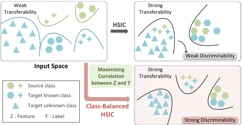
Reformulation of HSIC for OSDA. HSIC, as a norm of the covariance operator in Hilbert space, can be used as a correlation indicator. In OSDA problems, the separation of known classes from unknown classes is a very important goal. So when modeling with correlation metrics, separation between classes also needs to be ensured. To ensure that HSIC is applicable to OSDA, we reformulate HSIC in this section. As shown in Fig. 2, using the theoretical results, we can improve HSIC to make the learned features more discriminative. Let D := {(x1, y1), · · · , (xn, yn)} contain n i.i.d. samples drawn from PXY . Given separable RKHSs H, G, then the empirical expression of HSIC takes the following form [Gretton et al., 2005]:
where KX ∈ Rn×n , KY ∈ Rn×n with entries KX(i, j) = k(xi, xj), KY (i, j) = k(yi, yj), and H ∈ Rn×n is the centering matrix H = In - 1n 1n1Tn . In fact, with an appropriate kernel choice such as the Gaussian k(x, y) ∼ exp(- 12 ∥x - y∥2 /σ2 ), KX defines the similarity or the opposite of the distance among xi. Define the following adjacency matrix:
Next, Eq. (1) can be rewritten as follows:
Thus it is only necessary to analyze the adjacency matrixW to determine the learning direction. For the adjacency matrix, we derive the following theorem. The proof is provided in the appendix, fromwhich it is shown that this theorem can be similarly extended to other universal kernel function.
Theorem 1. Suppose the number of classes in D is c, and the proportion of each class is pi(i = 1, .., c), then when yi = yj and xi belongs to the t-th class, for Eq. (2) we have:
When yi ̸= yj and xi belongs to class a and xj belongs to class b, for Eq. (2) we have:
From the above theorem, HSIC is reformulated as the nodes' relation on graph, based on which we can know that the graph structure of HSIC is determined by the adjacency weights. Furthermore, the adjacency weights are mainly divided into two types: intra-class and inter-class, and are determined by the label prior, i.e., class ratio.
Separability of HSIC. For the correlation metric, when we enhance the correlation between features and labels, we want to achieve both separation between different classes. To achieve this, using the graph embedding theory of HSIC described above, we have the following definition:
Definition 1 (Separability). The HSIC meets the separation property if it satisfies that:
(a) The intra-class adjacency weight is positive, i.e., Wij > 0 for any yi = yj .
(b) The inter-class adjacency weight is negative, i.e., Wij < 0 for any yi ̸= yj.
With the separation property, we can enhance the correlation between feature and label while clustering samples from the same class and separating samples from different classes. Next, by considering the class ratio as variable, we can derive a sufficient condition for separability of HSIC. For samples of the same class, from Eq. (4), we have:
From this inequality, we can get the following inference.
Corollary 1. When yi = yj and xi belongs to the t-th class, then Wij > 0 and the adjacency weights Wij are determined by their corresponding class proportions pt.
From the above inference, we can know that when we increase the correlation between features and labels by maximizing HSIC(x, y), since KX defines the negative distance between features, and the intra-class adjacency weight is greater than 0, samples of the same class will be unconditionally narrowed, thus ensuring the intra-class compactness of features. While for samples belonging to different classes, from Eq. (5) we can know that maximising HSIC(x, y) will bring samples belonging to different classes closer together when the class proportions are out of balance. For OSDA
problems, the proportion of unknown classes is often large and the proportion of certain known classes is small, which makes the application of HSIC(x, y) to OSDA weaken the discriminability of the features and is not conducive to the optimisation of the model. From Thm. 1 we can see that the inter-class adjacency weights are determined by the class proportions, and from that point, in order to make all inter-class adjacency weight negative, we explore the nature of the HSIC when the class proportions are balanced. For Eq. (5), when the class proportions are balanced, we have:
So for samples belonging to different classes, we can obtain the following conclusion.
Corollary 2. When the class ratios are balanced, i.e., uniform label prior p = 1c 1c, and yi ̸= yj , then Wij < 0.
From the above corollaries, we can learn that class balance is a sufficient condition for separability. In addition, when the class ratios are balanced, the adjacency weights for each class will be equal, and will not result inWij in Eq. (4) getting smaller values in classes with larger class proportions.
Class-Balanced HSIC. Using the above analytical results, this paper designs class-balanced HSIC for OSDA. In the calculation of HSIC, the empirical distribution of samples in the empirical form of HSIC is p = 1n ∑i δxi . To allow HSIC to be computed on a class-balanced dataset, we weight the empirical distributions of the samples so that the class proportions are balanced. At this moment the weight of sample xi is 1 cnpi , where n is the total number of samples and pi is the proportion of class corresponding to yi. The HSIC calculated after the samples have been weighted is as follows:
where A = diag(a) - aaT . a ∈ Rn and a(i) is the weight corresponding to sample xi. By weighting the HSIC, we can achieve the effect of class balancing. In this case, the classbalanced HSIC meets the separation property. And we can enhance the discriminability of the features while preserving the statistical property of HSIC. Unlike [Wang et al., 2021b], we do not destroy the metric nature of the tools used.
To extract domain invariant features, similar to [Ma et al., 2020], we add class-balanced HSIC to the information bottleneck [Tishby et al., 2000]. The balanced HSIC bottleneck is used to extract domain invariant features:
The above balanced HSIC bottleneck is carried out on the basis of class balancing, which achieves the extraction of domain-invariant and class-discriminative features.
3.2 Class Conditional HSIC
To better align features of known classes in both domain, we implement cross-domain learning of the model in terms of conditional independence. Similar to [Fukumizu et al., 2007], we consider the form of the conditional HSIC. We can assess conditional independence between variables by the conditional cross-covariance operator VY X|Z = VY X - VY ZVZX . Similar to the definition of HSIC, the conditional HSIC can be defined as the operator norm of VYX|Z. Since we are trying to preserve the discriminative information in the aligned source and target domains, the corresponding conditional HSIC should be HSIC(Z,D|Y ). Since the values of Y are discrete and finite, we consider conditional HSIC based on the class slice form. In addition, the slice-based form also reduces the effect of class proportions on the experimental results while preserving the class information when aligning the source and target domain. The form of HSIC(Z,D|Y ) based on class slicing is as follows:
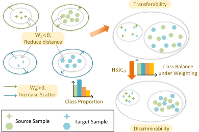
where Zi contains the features of the samples belonging to the i-th class, and Di is the set consisting of the domain labels corresponding to the samples in Zi. We achieve domain alignment by minimising the above loss to enable strong independence between sample features and domains in each class. As shown in Fig. 3, using the result of Thm. 1, we can also revisit the loss Eq. (10) in terms of graph embedding. In the process of minimizing LC, due to the existence of only two domains in the OSDA problem, for Eq. (5), we have:
where p1 and p2 are the ratios of source and target domain samples. This means that the same class samples between different domains are brought closer together and the scatter of the samples of the same class within the domain will be increased. Similar to [Xu et al., 2019], alignment of the samples in each class is achieved by allowing the samples of the same class within the domain to maintain a certain degree of scatter that can facilitate the model to mix the samples from different domains more evenly, which can be verified by our experiments. When samples of the same class in two domains can be uniformly mixed, the decision boundaries of the source domain model can apply well to the target domain data. Meanwhile, the final learned features of each class can also maintain a certain tightness due to the presence of LHB.
3.3 BCL for OSDA
Uncertainty-Based Identification. In the OSDA problem, the identification of unknown classes is crucial to achieve open set domain adaptation. Since our method guarantees a strong correlation between the features and labels of known class samples, the uncertainty of the known class samples is weak. In contrary, since the correlation of the unknown class samples is not guaranteed and there are no unknown class of samples in the source domain to be trained, it can be assumed that the unknown class samples possess a strong uncertainty. The relationship between entropy and uncertainty has been well studied in traditional statistics [Seidenfeld, 1987], so we utilise entropy in this section to achieve identification of unknown classes. The uncertainty measure based on entropy can then identify the unknown class samples with strong uncertainty. Denote the corresponding probability vector for xi as qi and the entropy can be calculated as follows:
For Ei, we can assume that larger values represent greater the uncertainty of the sample. So in this paper, we use entropy as the basis for identifying the unknown classes. Unlike other methods that rely on threshold setting, we use a clustering algorithm on Ei to classify the samples into three sets XL, XM, XH. Assuming that there are three class centres obtained from the clustering results as c1 > c2 > c3, then
XL denotes samples with low entropy values, i.e., samples with high confidence, generally representing samples that are clearly identified as known classes or unknown classes. XM denotes samples with medium confidence and can represent samples that are relatively close to the decision boundary. XH denotes samples with high uncertainty and can represent samples that are detached from the respective decision boundary. So, we treat XH as unknown classes. Regarding the set XH, we design the following cross-entropy function for unknown classes to ensure the recognition rate of the unknown classes:
where nu is the total number of samples in the set XH and qi(k+1) denotes the value of the predicted probability vector for the i-th sample in XH in the (k + 1)-th dimension. We achieve the identification of unknown classes by minimizing the cross-entropy of XH and continuously adding samples that are out of the decision boundary to unknown classes. This process avoids the setting of threshold and the interference of the number of unknown classes clustering structures.
Overall Flow of the Algorithm. The exact flow of the algorithm is shown in Alg. 1. In the pre-training phase, we train the model using the following cross-entropy loss:
where ˆ ys j = C(g(xsj )) and ∑k+1 i=1 ˆ ys j (i) = 1. ˆ ys j (i) is the prediction probability of xsj belonging to the i-th class. ys j is
Algorithm 1 Balanced Correlation Learning for OSDA
Input: Source Xs = {(xsi , ys i )}ns i=1 , target Xt = {xti }nt i=1 Parameter: regular term coefficient (α, β), β1 and β2, maximum iteration N, Pre-training iteration Npre
Output: Network parameters (Wg,WC) and predictions of target domain samples {ˆytj }nt j=1
- 1: for t = 1, . . . ,Npre do
- 2: Update the parameter of g and C following Eq. (15).
- 3: end for
- 4: for t = 1, . . . , (N -Npre) do
- 5: Calculate the entropy of the target domain samples using Eq. (12) and get the set XL,XM,XH.
- 6: Use the set XH to compute the loss LU.
- 7: Use the output of the classifier to label the samples in the set {XL, XM}, and calculate the loss LHB together with the source domain samples.
- 8: Take the known class samples in {XL,XM} and calculate loss LC together with the source domain samples.
- 9: Update the parameter of g and C following Eq. (16).
- 10: end for
the ground truth label of xsj . After the pre-training phase, the overall optimization objective is shown below:
4 Experiments
We evaluate our method on three datasets, i.e., Office31 [Saenko et al., 2010], Office-Home [Venkateswara et al., 2017] and VisDA [Peng et al., 2017]. BCL is compared with: (1) OSDA methods: OSBP [Saito et al., 2018], STA [Liu et al., 2019], PGL [Luo et al., 2020], ROS [Bucci et al., 2020], cUADAL [Jang et al., 2022], ANNA [Li et al., 2023]; (2) UniDA method: DANCE [Saito et al., 2020], GCL [Qu et al., 2023]. The results of the experiments were all averaged over five randomised trials. Details of datasets and implementations are provided in appendix.
4.1 Results and Analysis
Office-31. Comparison results on Office-31 are shown in Tab. 1. As shown in Tab. 1, our method achieves the best average UNK (93.0%) and HOS (92.1%) over all 6 tasks, outperforming STA, ROS and ANNA with 28.2%, 7.2% and 3.0% UnK and 19.6%, 6.2% and 3.5% HOS, respectively. Compared with the state-of-the-art OSDA work ANNA, our method comprehensively surpasses it with 3.7% OS∗ , 3.0% UnK and 3.5% HOS, respectively. In addition, our method outperforms other algorithms in terms of HOS metrics for all six tasks on Office-31, which verify the effect of our method. Office-Home. We report the comparison results of OfficeHome in Tab. 2. Our method achieves the best results in 4 sub-tasks for the HOS comparison and outperforming STA and ROS with 14.3% and 4.5% UnK and 8.7% and 4.4% HOS, respectively. Compared to the latest UniDA method GCL, our method outperforms by 0.8% in average HOS. Compared to the latest OSDA method ANNA, Our method also outperforms the previous best result with 70.8% HOS. VisDA. The comparative results of VisDA are shown at the end of Tab. 2. Our method achieves the best UNK (94.4%) and HOS (74.1%), outperforming STA, DANCE and cUADAL with 12.0%, 21.5% and 6.8% UnK and 3.1%, 7.6% and 4.0% HOS, respectively. Our method also outperforms the previous best result with 74.1% HOS.
| Method | A→W | A→D | D→A | D→W | W→A | W→D | Avg | ||||||||||||
|---|---|---|---|---|---|---|---|---|---|---|---|---|---|---|---|---|---|---|---|
| OS* | UnK | H OS* | UnK | H | OS* | UnK | H | OS* | UnK | H OS* | UnK | H | OS* UnK | H OS* | UnK | H | |||
| OSBP | 86.8 | 79.2 | 82.7 90.5 | 75.5 | 82.4 | 76.1 | 72.3 | 75.1 | 97.7 | 96.7 | 97.2 73.0 | 74.4 | 73.7 | 99.1 84.2 | 91.1 | 87.2 | 80.4 | 83.7 | |
| STA | 86.7 | 67.6 | 75.9 91.0 | 63.9 | 75.0 | 83.1 | 65.9 | 73.2 | 94.1 | 55.5 | 69.8 66.2 | 68.0 | 66.1 | 84.9 | 67.8 | 75.2 | 84.3 | 64.8 | 72.5 |
| PGL | 82.7 | 67.9 | 74.6 82.1 | 65.4 | 72.8 | 80.6 | 61.2 | 69.5 | 87.5 | 68.1 | 76.5 80.8 | 61.8 | 70.1 | 82.8 | 64.0 | 72.2 82.7 | 64.7 | 72.6 | |
| ROS | 88.4 | 76.7 | 82.1 87.5 | 77.8 | 82.4 | 74.8 | 81.2 | 77.9 | 99.3 | 93.0 | 96.0 69.7 | 86.6 | 77.2 | 100 | 99.4 | 99.7 | 86.6 | 85.8 | 85.9 |
| DANCE | 98.7 | 50.7 | 66.9 96.5 | 55.9 | 70.7 | 85.3 | 53.6 | 65.8 | 100 | 66.8 | 80.0 83.7 | 60.6 | 70.2 | 100 | 73.7 | 84.8 94.0 | 60.2 | 73.1 | |
| cUADAL | 85.5 | 95.1 | 90.1 85.6 | 90.4 | 87.9 | 74.2 | 87.8 | 80.5 | 98.7 | 97.7 | 98.2 65.6 | 87.8 | 75.1 | 99.3 | 99.4 | 99.4 84.8 | 93.0 | 88.5 | |
| GCL | - | - | - - | - | - | - | - | - | - | - | - - | - | - | - | - | - - | - | 89.0 | |
| ANNA | 82.8 | 88.4 | 85.5 93.2 | 76.1 | 83.8 | 75.4 | 91.1 | 82.5 | 99.4 | 99.6 | 99.5 76.0 | 87.9 | 81.6 | 100 96.8 | 98.4 87.8 | 90.0 | 88.6 | ||
| BCL | 95.6 | 89.4 | 92.4 91.5 | 85.3 | 88.3 | 81.1 | 89.0 | 84.8 | 99.4 | 99.6 | 99.5 80.2 | 94.8 | 86.9 | 99.3 100 | 99.7 | 91.2 | 93.0 | 92.1 | |
| Method | Ar→Cl | Ar→Pr | Ar→Rw | Cl→Ar | Cl→Pr | Cl→Rw | Pr→Ar | |||||||||||||||
|---|---|---|---|---|---|---|---|---|---|---|---|---|---|---|---|---|---|---|---|---|---|---|
| OS* | UnK | H | OS* | UnK | H | OS* | UnK | H OS* | UnK | H | OS* | UnK | H | OS* | UnK | H | OS* | UnK | H | |||
| OSBP | 50.2 | 61.1 | 55.1 | 71.8 | 59.8 | 65.2 | 79.3 | 67.5 | 72.9 59.4 | 70.3 | 64.3 | 67.0 | 62.7 | 64.7 | 72.0 | 69.2 | 70.6 | 59.1 | 68.1 | 63.2 | ||
| STA | 50.8 | 63.4 | 56.3 | 68.7 | 59.7 | 63.7 | 81.1 | 50.5 | 62.1 53.0 | 63.9 | 57.9 | 61.4 | 63.5 | 62.5 | 69.8 | 63.2 | 66.3 | 55.4 | 73.7 | 63.1 | ||
| PGL | 63.3 | 19.1 | 29.3 | 78.9 | 32.1 | 45.6 | 87.7 | 40.9 | 55.8 85.9 | 5.3 | 10.0 | 73.9 | 24.5 | 36.8 | 70.2 | 33.8 | 45.6 | 73.7 | 34.7 | 47.2 | ||
| ROS | 50.6 | 74.1 | 60.1 | 68.4 | 70.3 | 69.3 | 75.8 | 77.2 | 76.5 53.6 | 65.5 | 58.9 | 59.8 | 71.6 | 65.2 | 65.3 | 72.2 | 68.6 | 57.3 | 64.3 | 60.6 | ||
| DANCE | 54.4 | 53.7 | 53.1 | 84.0 | 35.4 | 49.8 | 89.8 | 25.3 | 39.4 72.9 | 28.4 | 40.9 | 76.3 | 32.8 | 45.9 | 83.9 | 18.4 | 30.2 | 70.7 | 43.9 | 54.2 | ||
| cUADAL | 55.0 | 75.6 | 63.6 | 69.4 | 73.9 | 71.6 | 82.2 | 73.3 | 77.5 53.8 | 82.0 | 65.0 | 61.1 | 77.4 | 68.3 | 69.3 | 76.3 | 72.6 | 50.9 | 82.4 | 62.9 | ||
| GCL | - | - | 65.3 | - | - | 74.2 | - | - | - | - | 60.4 | - | - | 71.6 | - | - | 74.7 | - | - | 63.7 | ||
| ANNA | 61.4 | 78.7 | 69.0 | 68.3 | 79.9 | 73.7 | 74.1 | 79.7 | 79.0 76.8 58.0 | 73.1 | 64.7 | 64.2 | 73.6 | 68.6 | 66.9 | 80.2 | 73.0 | 63.0 | 70.3 | 66.5 | ||
| BCL | 56.6 | 74.3 | 64.3 | 71.8 | 79.5 | 75.4 | 77.0 | 81.2 | 79.0 57.1 | 70.8 | 63.1 | 64.7 | 76.3 | 70.0 | 70.0 | 77.1 | 73.4 | 62.1 | 70.8 | 66.2 | ||
| Method | Pr→Cl | Pr→Rw | Rw→Ar | Rw→Cl | Rw→Pr | Avg | VisDA | |||||||||||||||
| OS* | UnK | H | OS* | UnK | H | OS* | UnK | H OS* | UnK | H | OS* | UnK | H | OS* | UnK | H | OS* | UnK | H | |||
| OSBP | 44.5 | 66.3 | 53.2 | 76.2 | 71.7 | 73.9 | 66.1 | 67.3 | 66.7 48.0 | 63.0 | 54.5 | 76.3 | 68.6 | 72.3 | 64.1 66.3 | 64.7 | 50.9 | 81.7 | 62.7 | |||
| STA | 44.7 | 71.5 | 55.0 | 78.1 | 63.3 | 69.7 | 67.9 | 62.3 | 65.0 51.4 | 57.9 | 54.2 | 77.9 | 58.0 | 66.4 | 63.4 | 62.6 | 61.9 | 62.4 | 82.4 | 71.0 | ||
| PGL | 59.2 | 38.4 | 46.6 | 84.8 | 27.6 | 41.6 | 81.5 | 6.1 | 11.4 68.8 | 0.0 | 0.0 | 84.8 | 38.0 | 52.5 | 76.1 | 25.0 | 35.2 | - | - | - | ||
| ROS | 46.5 | 71.2 | 56.3 | 70.8 | 78.4 | 74.4 | 67.0 | 70.8 | 68.8 51.5 | 73.0 | 60.4 | 72.0 | 80.0 | 75.7 | 61.6 | 72.4 | 66.2 | 45.8 | 64.8 | 53.7 | ||
| DANCE | 48.2 | 67.4 | 55.7 | 86.5 | 27.1 | 41.2 | 79.2 | 16.7 | 27.5 60.1 | 41.3 | 48.3 | 86.2 | 29.6 | 44.0 | 74.4 | 35.0 | 44.2 | 61.3 | 72.9 | 66.5 | ||
| cUADAL | 41.2 | 80.7 | 54.6 | 71.2 | 83.4 | 76.8 | 66.8 | 79.6 | 72.6 51.8 | 71.1 | 59.9 | 77.8 | 75.6 | 76.7 | 62.5 | 77.6 | 68.5 | 58.5 | 87.6 | 70.1 | ||
| GCL | - | - | 63.2 | - | - | 75.8 | - | - | 67.1 - | - | 64.3 | - | - | 77.8 | - | - | 69.8 | - | - | 72.5 | ||
| ANNA | 54.6 | 74.8 | 63.1 | 74.3 | 78.9 | 76.6 | 66.1 | 77.3 | 71.3 59.7 | 73.1 | 65.7 | 76.4 | 81.0 | 78.7 | 65.6 76.7 | 70.7 | - | - | - | |||
| BCL | 54.5 | 73.5 | 62.5 | 74.0 | 81.0 | 77.3 | 63.3 | 77.6 | 69.7 56.9 | 75.1 | 64.7 | 77.9 | 86.7 | 82.1 | 65.5 | 77.0 | 70.8 | 60.9 | 94.4 | 74.1 | ||
Ablation Study: As shown in Tab 3, we performed ablation studies on four sub-tasks on Office-Home and obtain the following observations. 1) When only using the HSIC bottleneck to increase the correlation between features and labels, the average HOS reduced by 1.8%, which is mainly caused by the decrease in the unknown class recognition rate. This indicates that when two domains are not well aligned, the HSIC bottleneck discards the discriminative information related to the unknown class, which leads to the degradation of the unknown class recognition. 2) When only using slicing HSIC to align both domains, the average HOS increased by 3.6%, which shows that even though this module increases the intraclass scatter, a better identification result can still be achieved with the cross entropy of the source domain.
Hyper-parameter Sensitivity: The results of the parameter sensitivity are shown in Fig. 4. The values of the four parameters have a small effect on the HOS, which indicates that our algorithm is stable. The values of β and β1 also have a smaller effect on the recognition effectiveness of the unknown class, in contrast to the values of α and β2, which have a larger effect on the recognition rate of the unknown class, although this effect also leads to variations in the recognition effectiveness of the known class, thus maintaining a stable HOS.
Feature Visualization: We take W→A for instance and plot the t-SNE results in Fig. 5 to visualize the feature distribution and make a comparison for different methods. From Fig. 5, in contrast to other methods, our method separates each class to ensure feature discriminability. In addition, BCL will mix the samples of the same class from different domains more evenly, as evidenced by the fact that the same class samples from both domain will be evenly mixed. On the contrary, other methods simply put the clustering structures belonging to the same class in the source and target domains next to each other, and cannot form a homogeneously mixed whole.
| LHB | Ar→Pr | Pr→Cl | Cl→Rw | Rw→Ar | Avg | ||||||||||
|---|---|---|---|---|---|---|---|---|---|---|---|---|---|---|---|
| OS* | UnK | H | OS* | UnK | H | OS* | UnK | H | OS* | UnK | H | OS* | UnK | H | |
| 63.2 | 81.2 | 71.0 | 46.1 | 65.4 | 54.0 | 58.8 | 75.5 | 66.0 | 60.6 | 81.9 | 69.6 | 57.2 | 76 | 65.2 | |
| 65.8 | 64.9 | 65.4 | 46.4 | 62.2 | 53.1 | 58.0 | 77.0 | 66.1 | 61.0 | 79.5 | 69.0 | 57.8 | 70.9 | 63.4 | |
| 71.2 | 75.3 | 73.2 | 54.1 | 68.2 | 60.3 | 66.8 | 78.4 | 72.1 | 64.2 | 76.1 | 69.6 | 60.1 | 74.5 | 68.8 | |
| 71.8 | 79.5 | 75.4 | 54.5 | 73.5 | 62.5 | 70.0 | 77.1 | 73.4 | 63.3 | 77.6 | 69.7 | 64.9 | 76.9 | 70.3 | |
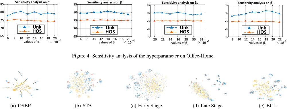
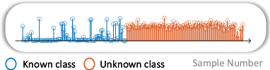
Validation of Theory: To verify the accuracy of our theory, we conducted experiments with unweighted HSIC. In (c) and (d) of Fig. 5 we can see the visualisation results of using unweighted HSIC. As shown in (c), in early stage of the algorithm, there are few samples that are explicitly recognised as unknown classes, so it leads to many known class samples mixed with unknown class samples. This results in more known class samples being mixed with unknown class samples in the late stage of the algorithm, and the separability between different classes cannot be achieved, as shown in (d). Unknown Class Identification: To verify the reliability of the operation of using entropy to identify unknown classes, we conducted numerical experiments on W→A (Office-31). The results are shown in Fig. 6. From the figure, we can see that although the entropy of some of the known classes will be larger resulting in a small portion of the known classes being recognized as unknown classes, basically the entropy of the unknown classes is large, which explains the high accuracy of the unknown class recognition of our algorithm.
5 Conclusion
In this work, we establish the relationship between HSIC and graph embedding, based on which we propose a framework for OSDA based on correlation metric, called BCL. BCL establishes the correlation between feature and label, in which the class-balanced HSIC ensures the class-discriminative nature of features while extracting domain-invariant features. Furthermore, to better align both domains from conditional independence, the conditional HSIC based on class slicing implements a class-by-class alignment. Once the correlation between feature and label is established, we can use entropy to measure the uncertainty of the samples, thus enabling the identification of unknown classes. Extensive experiments on standard benchmarks verify its state-of-the-art performance.
Acknowledgments
This work was supported in part by National Natural Science Foundation of China (Grant No.62376291), in part by Guangdong Basic and Applied Basic Research Foundation (2023B1515020004), and in part by Science and Technology Program of Guangzhou (2024A04J6413).
@inproceedings{ijcai2024p98,
  title     = {Rethinking Correlation Learning via Label Prior for Open Set Domain Adaptation},
  author    = {Huang, Zi-Xian and Ren, Chuan-Xian},
  booktitle = {Proceedings of the Thirty-Third International Joint Conference on
               Artificial Intelligence, {IJCAI-24}},
  publisher = {International Joint Conferences on Artificial Intelligence Organization},
  editor    = {Kate Larson},
  pages     = {884--892},
  year      = {2024},
  month     = {8},
  note      = {Main Track},
  doi       = {10.24963/ijcai.2024/98},
  url       = {https://doi.org/10.24963/ijcai.2024/98},
}
TY - CPAPER TI - Rethinking Correlation Learning via Label Prior for Open Set Domain Adaptation AU - Huang, Zi-Xian AU - Ren, Chuan-Xian T2 - Proceedings of the Thirty-Third International Joint Conference on Artificial Intelligence, IJCAI-24 PB - International Joint Conferences on Artificial Intelligence Organization PY - 2024 SP - 884 EP - 892 DO - 10.24963/ijcai.2024/98 UR - https://doi.org/10.24963/ijcai.2024/98 ER -Copied
Machine-readable versions of this paper, for tools and AI agents:





