
Towards Comprehensive and Prerequisite-Free Explainer for Graph Neural Networks
Proceedings of the Thirty-Fourth International Joint Conference on Artificial Intelligence. AI4Tech: AI Enabling Technologies. Pages 9456-9464.
https://doi.org/10.24963/ijcai.2025/1051
Keywords
- Advanced AI4Tech: AI4Tech foundations
- Domain-specific AI4Tech: AI4Safety
- Emerging AI4Tech: Ethical and responsible AI4Tech
Abstract
To enhance the reliability and credibility of graph neural networks (GNNs) and improve the transparency of their decision logic, a new field of explainability of GNNs (XGNN) has emerged. However, two major limitations severely degrade the performance and hinder the generalizability of existing XGNN methods: they (a) fail to capture the complete decision logic of GNNs across diverse distributions in the entire dataset's sample space, and (b) impose strict prerequisites on edge properties and GNN internal accessibility. To address these limitations, we propose OPEN, a novel cOmprehensive and Prerequisite-free Explainer for GNNs. OPEN, as the first work in the literature, can infer and partition the entire dataset's sample space into multiple environments, each containing graphs that follow a distinct distribution. OPEN further learns the decision logic of GNNs across different distributions by sampling subgraphs from each environment and analyzing their predictions, thus eliminating the need for strict prerequisites. Experimental results demonstrate that OPEN captures nearly complete decision logic of GNNs, outperforms state-of-the-art methods in fidelity while maintaining similar efficiency, and enhances robustness in real-world scenarios.
- [Agarwal et al., 2023] Chirag Agarwal, Owen Queen, Himabindu Lakkaraju, and Marinka Zitnik. Evaluating explainability for graph neural networks. Scientific Data, 10(1):144, 2023.
- [Ahuja et al., 2021] Kartik Ahuja, Ethan Caballero, Dinghuai Zhang, Jean-Christophe Gagnon-Audet, Yoshua Bengio, Ioannis Mitliagkas, and Irina Rish. Invariance principle meets information bottleneck for out-of-distribution gener- alization. In NeurIPS, volume 34, pages 3438-3450, 2021.
- [Amara et al., 2022] Kenza Amara, Zhitao Ying, Zitao Zhang, Zhihao Han, Yinan Shan, Ulrik Brandes, and Sebas- tian Schemm. Graphframex: Towards systematic evaluation of explainability methods for graph neural networks. In NeurIPS Workshop, 2022.
- [Chen et al., 2022] Yongqiang Chen, Yonggang Zhang, Yatao Bian, Han Yang, MA Kaili, Binghui Xie, Tongliang Liu, Bo Han, and James Cheng. Learning causally invariant representations for out-of-distribution generalization on graphs. In NeurIPS, volume 35, pages 22131-22148, 2022.
- [Chen et al., 2023] Jialin Chen, Shirley Wu, Abhijit Gupta, and Rex Ying. D4explainer: in-distribution gnn explana- tions via discrete denoising diffusion. In NeurIPS, pages 78964-78986, 2023.
- [Chen et al., 2024a] Yongqiang Chen, Yatao Bian, Bo Han, and James Cheng. How interpretable are interpretable graph neural networks? In ICML, 2024.
- [Chen et al., 2024b] Zhuomin Chen, Jiaxing Zhang, Jingchao Ni, Xiaoting Li, Yuchen Bian, Md Mezbahul Islam, Ananda Mondal, Hua Wei, and Dongsheng Luo. Generating in- distribution proxy graphs for explaining graph neural net- works. In ICML, 2024.
- [Ding et al., 2025] Pengfei Ding, Yan Wang, Guanfeng Liu, Nan Wang, and Xiaofang Zhou. Few-shot causal repre- sentation learning for out-of-distribution generalization on heterogeneous graphs. TKDE, 37(4):1804-1818, 2025.
- [Fang et al., 2024a] Junfeng Fang, Wei Liu, Yuan Gao, Zemin Liu, An Zhang, Xiang Wang, and Xiangnan He. Evaluating post-hoc explanations for graph neural networks via robustness analysis. In NeurIPS, volume 36, 2024.
- [Fang et al., 2024b] Junfeng Fang, Guibin Zhang, Kun Wang, Wenjie Du, Yifan Duan, Yuankai Wu, Roger Zimmermann, Xiaowen Chu, and Yuxuan Liang. On regularization for explaining graph neural networks: An information theory perspective. TKDE, 2024.
- [Fey and Lenssen, 2019] Matthias Fey and Jan E. Lenssen. Fast graph representation learning with PyTorch Geometric. In ICLR Workshop, 2019.
- [Golmaei and Luo, 2021] Sara Nouri Golmaei and Xiao Luo. Deepnote-gnn: predicting hospital readmission using clin- ical notes and patient network. In ACM-BCB, pages 1-9, 2021.
- [Gui et al., 2022] Shurui Gui, Xiner Li, Limei Wang, and Shuiwang Ji. Good: A graph out-of-distribution benchmark. In NeurIPS, volume 35, pages 2059-2073, 2022.
- [Kawamoto et al., 2018] Tatsuro Kawamoto, Masashi Tsub- aki, and Tomoyuki Obuchi. Mean-field theory of graph neural networks in graph partitioning. In NeurIPS, vol- ume 31, 2018.
- [Kingma and Welling, 2014] Diederik P Kingma and Max Welling. Auto-encoding variational bayes. stat, 1050:1, 2014.
- [Koch et al., 2022] Lisa M Koch, Christian M Schürch, Arthur Gretton, and Philipp Berens. Hidden in plain sight: Subgroup shifts escape ood detection. In Machine Learning Research, volume 172, pages 726-740. PMLR, 2022.
- [Koch et al., 2024] Lisa M Koch, Christian F Baumgartner, and Philipp Berens. Distribution shift detection for the postmarket surveillance of medical ai algorithms: a retro- spective simulation study. NPJ Digital Medicine, 7(1):120, 2024.
- [Kubo and Difallah, 2024] Ryoji Kubo and Djellel Difallah. Xgexplainer: Robust evaluation-based explanation for graph neural networks. In SDM, pages 64-72. SIAM, 2024.
- [Li et al., 2022] Michelle M Li, Kexin Huang, and Marinka Zitnik. Graph representation learning in biomedicine and healthcare. Nature Biomedical Engineering, 6(12):1353- 1369, 2022.
- [Liu et al., 2021] Meng Liu, Youzhi Luo, Limei Wang, Yaochen Xie, Hao Yuan, Shurui Gui, Haiyang Yu, Zhao Xu, Jingtun Zhang, Yi Liu, Keqiang Yan, Haoran Liu, Cong Fu, Bora M Oztekin, Xuan Zhang, and Shuiwang Ji. DIG: A turnkey library for diving into graph deep learning research. Journal of Machine Learning Research, 22(240):1-9, 2021.
- [Lucic et al., 2022] Ana Lucic, Maartje A Ter Hoeve, Gabriele Tolomei, Maarten De Rijke, and Fabrizio Silvestri. Cf-gnnexplainer: Counterfactual explanations for graph neural networks. In AISTATS, pages 4499-4511. PMLR, 2022.
- [Luo et al., 2020] Dongsheng Luo, Wei Cheng, Dongkuan Xu, Wenchao Yu, Bo Zong, Haifeng Chen, and Xiang Zhang. Parameterized explainer for graph neural network. In NeurIPS, volume 33, pages 19620-19631.
- [Miller et al., 2020] David J Miller, Zhen Xiang, and George Kesidis. Adversarial learning targeting deep neural network classification: A comprehensive review of defenses against attacks. In IEEE, volume 108, pages 402-433. IEEE, 2020.
- [Min et al., 2024] Xin Min, Wei Li, Ruiqi Han, Tianlong Ji, and Weidong Xie. Graph neural collaborative filtering with medical content-aware pre-training for treatment pattern recommendation. Pattern Recognition Letters, 185:210- 217, 2024.
- [Pope et al., 2019] Phillip E. Pope, Soheil Kolouri, Moham- mad Rostami, Charles E. Martin, and Heiko Hoffmann. Explainability methods for graph convolutional neural net- works. In IEEE/CVF CVPR, pages 10772-10781, 2019.
- [Qiu et al., 2024] Dazhuo Qiu, Mengying Wang, Arijit Khan, and Yinghui Wu. Generating robust counterfactual witnesses for graph neural networks. arXiv preprint arXiv:2404.19519, 2024.
- [Simonovsky and Komodakis, 2018] Martin Simonovsky and Nikos Komodakis. Graphvae: Towards generation of small graphs using variational autoencoders. In ICANN, pages 412-422. Springer, 2018.
- [Togninalli et al., 2019] Matteo Togninalli, Elisabetta Ghisu, Felipe Llinares-López, Bastian Rieck, and Karsten Borg- wardt. Wasserstein weisfeiler-lehman graph kernels. In NeurIPS, volume 32, 2019.
- [Veličković et al., 2018] Petar Veličković, Guillem Cucu- rull, Arantxa Casanova, Adriana Romero, Pietro Lio, and Yoshua Bengio. Graph attention networks. stat, 1050(20):10-48550, 2018.
- [Vu and Thai, 2020] Minh Vu and My T Thai. Pgm-explainer: Probabilistic graphical model explanations for graph neural networks. In NeurIPS, volume 33, pages 12225-12235, 2020.
- [Wang and Shen, 2023] Xiaoqi Wang and Han Wei Shen. Gn- ninterpreter: A probabilistic generative model-level expla- nation for graph neural networks. In ICLR, 2023.
- [Wu et al., 2021] Yingxin Wu, Xiang Wang, An Zhang, Xi- angnan He, and Tat-Seng Chua. Discovering invariant rationales for graph neural networks. In ICLR, 2021.
- [Xiong et al., 2021] Kai Xiong, Xiao Ding, Li Du, Ting Liu, and Bing Qin. Heterogeneous graph knowledge enhanced stock market prediction. AI Open, 2:168-174, 2021.
- [Xu et al., 2024] Rongwei Xu, Guanfeng Liu, Yan Wang, Xuyun Zhang, Kai Zheng, and Xiaofang Zhou. Adaptive hypergraph network for trust prediction. In ICDE, pages 2986-2999. IEEE, 2024.
- [Ying et al., 2019] Zhitao Ying, Dylan Bourgeois, Jiaxuan You, Marinka Zitnik, and Jure Leskovec. Gnnexplainer: Generating explanations for graph neural networks. In NeurIPS, volume 32, pages 9244-9255.
- Curran Associates, Inc., 2019.
- [Yuan et al., 2020] Hao Yuan, Jiliang Tang, Xia Hu, and Shui- wang Ji. Xgnn: Towards model-level explanations of graph neural networks. In ACM KDD, pages 430-438, 2020.
- [Zhang et al., 2022] Wenjun Zhang, Zhensong Chen, Jianyu Miao, and Xueyong Liu. Research on graph neural network in stock market. Procedia Computer Science, 214:786-792, 2022.
- [Zhang et al., 2023] Jiaxing Zhang, Dongsheng Luo, and Hua Wei. Mixupexplainer: Generalizing explanations for graph neural networks with data augmentation. In ACM KDD, pages 3286-3296, 2023.
- [Zhu et al., 2023] Jiajie Zhu, Yan Wang, Feng Zhu, and Zhu Sun. Domain disentanglement with interpolative data aug- mentation for dual-target cross-domain recommendation. In RecSys, pages 515-527, 2023.
References were extracted automatically from the PDF and may contain errors.
Full text extracted automatically from the PDF; figures, tables and equations may differ. The PDF is the version of record.
1 Introduction
Graph neural networks (GNNs), known for their capability to learn complex relational patterns in graphs, have gained significant attention and been widely applied in critical fields such as finance [Zhang et al., 2022; Xu et al., 2024] and healthcare [Golmaei and Luo, 2021]. For example, in healthcare, GNNs can utilize information from patients and others with similar conditions to offer medical recommendations [Min et al., 2024]. However, because users in these fields require reliable and accurate GNN predictions, the lack of transparency in the decision logic of GNNs has raised significant concerns about the credibility of GNN predictions. To address these concerns, the field of explainability of GNNs (XGNN) has emerged to enhance the transparency of the decision logic of GNNs and build up users' trust in GNN predictions. Existing XGNN methods [Ying et al., 2019; Yuan et al., 2020; Vu and Thai, 2020] typically perturb the input graph structures to influence GNN predictions and extract the key subgraphs (a.k.a., explanation subgraphs) that are most critical to support these predictions. These subgraphs are expected to represent the decision logic of GNNs to a certain extent, thereby effectively enhancing the predictions' reliability.
∗Corresponding author
However, existing XGNN methods face two major limitations in real-world scenarios. Limitation 1 (Incomplete Decision Logic): Existing methods fail to capture the complete decision logic of GNNs across diverse distributions in the entire dataset's sample space, which overall may consist of all possible graph structures. These methods assume that the testing dataset (testing samples in the entire dataset) follows the same distribution as the training dataset (a.k.a., IID scenario) and focus solely on extracting the decision logic of GNNs in the training dataset. However, in real-world applications, out-of-distribution (OOD) scenarios are more prevalent [Koch et al., 2024; Koch et al., 2022], where the testing dataset's distribution differs from that of the training dataset. In such cases, existing XGNN methods fail to provide reliable explanations because they focus either on OOD explanations that have different distributions from the training dataset or on the IID scenario. This limitation raises the demand of a novel comprehensive GNN explainer, which needs to capture the complete decision logic of the target GNN across diverse distributions in the entire dataset's sample space and thus can: (1) generate reliable explanations in OOD scenarios, (2) help identify flaws in GNN decision logic when prediction errors occur, and (3) support GNN design improvements to mitigate errors in OOD scenarios. Limitation 2 (Strict Prerequisites): Existing XGNN methods rely on strict prerequisites to achieve good performance, which can be divided into two aspects: (1) Most methods require GNN internal accessibility to extract the decision logic of GNNs. However, privacy protection laws and regulations often restrict such access, making these methods impractical for privacy-sensitive applications [Miller et al., 2020]; (2) Several recent methods [Wang and Shen, 2023; Chen et al., 2024b] generate learnable edge weights and require GNNs to use these weights for weighted message propagation. However, in critical fields like finance and healthcare, edge features (e.g., stock investment shares in finance and co-occurrence frequency of medical services in healthcare) are used to enhance data representation [Li et al., 2022; Xiong et al., 2021; Zhu et al., 2023]. These edge features differ from learnable edge weights in both semantics and data formats, yet they share the same position in the input graph. Thus, these XGNN methods impose a prerequisite on dataset properties, requiring that datasets do not contain edge features.
To address the abovementioned two major limitations in existing XGNN methods, we propose OPEN, a novel cOmprehensive and Prerequisite-free Explainer for graph Neural networks. Specifically, we propose the Non-Parametric Analysis Framework (NPAF), which infers the entire dataset's sample space from the training dataset samples and partitions this space into multiple environments. In addition, we propose the Graph Variational Generator (GVAG), which determines the sampling probabilities of graph structures by generating a large number of subgraphs in each environment during the training stage and analyzing their predictions. This enables GVAG to uncover the decision logic of the GNNs across a wide range of distributions in the sample space. To further enhance this uncovering process, GVAG incorporates node embeddings from other environments to actively construct OOD data. Compared to existing methods, OPEN can capture nearly complete decision logic of the GNNs, effectively addressing Limitation 1. Moreover, GVAG learns the correlations between embeddings and structure sampling probabilities, and directly samples explanation subgraphs from the sample space without accessing GNN internals or using edge weights, thereby eliminating the prerequisites required by existing methods and overcoming Limitation 2.
We summarize our main contributions as follows: (1) We identify two major limitations in XGNN: (a) its inability to capture the complete decision logic, and (b) the strict prerequisites imposed on target GNNs and datasets. These limitations significantly impact XGNN research, highlighting the need for effective solutions; (2) We propose OPEN, a framework that infers and partitions the sample space of the entire dataset, enabling the exploration of the decision logic of GNNs across diverse distributions. In addition, OPEN learns the decision logic by sampling a large number of subgraphs and analyzing their predictions. This approach not only captures a more comprehensive decision logic than existing methods, but also removes the required strict prerequisites; and (3) Comprehensive experimental results demonstrate that OPEN not only effectively extracts explanation subgraphs in prerequisite-free scenarios where most existing methods are inapplicable, but also outperforms state-of-the-art (SOTA) methods in prerequisitesatisfied scenarios. OPEN efficiently generates reliable and accurate explanations across various distributions, showcasing its adaptability to real-world applications.
2 RelatedWork
XGNN. The XGNN methods are initially inspired by computer vision techniques like Grad-CAM [Pope et al., 2019], and some methods also benefit from the explanatory power of GNN attention mechanisms [Veliˇckovi´c et al., 2018]. The introduction of GNNExplainer [Ying et al., 2019] marked a shift towards perturbing graph structures to weight message propagation along edges and extracting explanation subgraphs based on changes in GNN outputs, as demonstrated by later advancements [Qiu et al., 2024; Chen et al., 2024b; Chen et al., 2024a]. However, most existing methods rely on strict prerequisites to enable graph structure perturbation, which often restricts their practicality in real-world scenarios. Techniques like PGExplainer [Luo et al., 2020] enhance the understanding of how node embeddings correlate with node presence in explanation subgraphs, facilitating explanations post-learning without the need for fitting new instances [Zhang et al., 2023]. Nevertheless, these methods focus on learning the decision logic in the training dataset and thus fail to mine the complete decision logic of target GNNs, which causes them to provide unrelated explanations when the distribution of the input graph is different from that of the training dataset.
OOD Scenarios in XGNN. In the XGNN field, critiques [Chen et al., 2023; Chen et al., 2024b; Fang et al., 2024a; Kubo and Difallah, 2024; Fang et al., 2024b] note that traditional methods generate OOD explanations, arguing that these explanations fail to accurately reflect the decision logic of GNNs. To address this issue, they propose generating explanations that align with the training dataset's distribution. However, this further aggravates the performance degradation of these methods in OOD scenarios. Some argue that an XGNN method only needs to be faithful to the decision logic of a well-trained GNN in the training dataset's distribution, and does not need to uncover the reasoning behind incorrect predictions in OOD scenarios. However, such opinion not only significantly limits the practical use of XGNN in critical fields where OOD scenarios are prevalent, but also prevents XGNN from contributing to improvements in GNN design.
3 Preliminaries
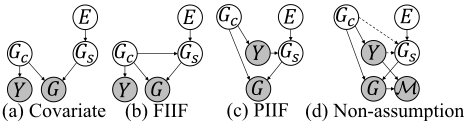
Structural Causal Models (SCMs). Following prior works [Ahuja et al., 2021; Chen et al., 2022; Ding et al., 2025], SCMs are used to delineate causal relationships among variables. Fig. 1 demonstrates three typical distribution shift assumptions in SCMs: Covariate, Fully Informative Invariant Features (FIIF), and Partially Informative Invariant Features (PIIF). Specifically, we propose a Non-assumption SCM (shown in Fig. 1 (d)), which primarily explores potential causal relationships among variables Gc, Y , and Gs. We can find that relying solely on Y and G is insufficient for precise causal analysis among these variables. Therefore, we perform direct statistical analyses to deduce environmental variables E and identify variables with distinct causal relationships to either Y or E, effectively isolating relevant subsets of Gc and Gs and reducing the impact of spurious correlations. In addition, the target GNN M has causal relationships with both G and Y , indicating that when an XGNN method explains M's output, M opens a backdoor path between the XGNN method and Y . Therefore, XGNN methods also learn the relationships between Y and Gc, and are susceptible to OOD scenarios.
Problem Definition. We focus on providing post-hoc instance-level explanations. Given a graph G = (V, E,X) where V denotes the vertices, E denotes the edges, and X is the node features, the target problem is defined as follows:
Definition 1 (Mining complete decision logic of GNNs). Given a GNN model M trained on the training dataset Dtrain, consider an unseen testing dataset Dtest where graphs exhibit distribution shifts from those in Dtrain. For each G ∈ Dtest, the objective is to identify an explanation subgraph Gc ⊆ G that effectively elucidates the predictions made by M.
Meanwhile, to eliminate the required prerequisites, we will not use learnable edge weights or access the GNN internal.
4 Methodology of OPEN
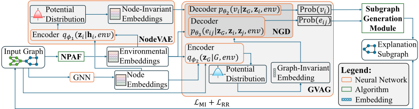
In this section, we present a novel framework, comprehensive and prerequisite-free explainer for GNNs (OPEN). Fig. 2 depicts the overview of OPEN. A summary of all symbols used in this paper is provided in Appendix A.1. OPEN uses the NonParametric Analysis Framework (NPAF) to analyze potential environments in the entire dataset's sample space, based on training dataset samples. NPAF employs statistical methods following the non-assumption SCM and assigns environmental labels to the graphs in the training dataset. Next, NodeVAE and the Graph Variational Generator (GVAG) generate node and graph invariant embeddings in each environment, respectively. GVAG then samples explanation subgraphs from the sample space based on these invariant embeddings. OPEN adjusts the sampling probability of explanations by comparing the predictions, thus uncovering the decision logic of GNNs. 1
4.1 NPAF for Environmental Label Inference
Taking the graph classification task as an example, NPAF determines the potential environmental label for each graph Gi ∈ Dtrain through the following procedure.
Obtain Structure-Based Embedding. NPAF leverages structure-based embeddings to infer environmental labels from the structural aspects of the training dataset. To generate these embeddings, we gather relevant structural information from the training dataset, such as node degrees and node categories.
1 Appendix can be found at https://github.com/zh2209645/OPEN
Using these details, we construct structure-based node features Xstr and apply a Weisfeiler Leman (WL) kernel-based GNNs [Togninalli et al., 2019] to derive the structure-based embeddings for nodes Hstr. We then employ pooling layers to extract the structure-based embedding hG,i ∈ HG for Gi.
Infer Potential Environmental Label Based on Structure. We infer potential environmental labels for graphs based on a commonly adopted assumption in this field [Wu et al., 2021; Chen et al., 2022], which states that a graph can be divided into two independent components: Gc, associated with the label Y , and Gs, influenced by the environment variable E. Graphs affected by the same E are expected to share similar connection patterns during generation. Thus, potential environmental labels E can be inferred by analyzing and classifying graph structures. To assign structure-based environmental labels, we apply the K-Means algorithm to cluster structure-based embeddings HG for Gi ∈ Dtrain. The number of clusters, K, determines the granularity of potential environments. A larger K indicates greater diversity and the presence of multiple potential environments, while a smaller K reflects less structural diversity. Based on the clustering results, each graph Gi is assigned an environmental label Es k ∈ Estr = {Es 1 , Es 2 , ..., EsK }.
Identify Causal Structure in Graphs. To identify nodes and edges in Gi that have a causal relationship with Es k , we leverage the idea that graphs influenced by the same E exhibit similar structural patterns. Specifically, structure-based embeddings of nodes belonging to the Gs should show higher similarity within the same environment. This is because the embeddings Hstr generated by the WL kernel effectively capture graph structures and reflect connection patterns. Since embeddings Hstr are highly correlated with E, they can be used to infer causal relationships between nodes and the environment. To pinpoint nodes irrelevant to the environment, we analyze the variance in their structure-based embeddings. For nodes sharing the same Es k and classification label Y within Dtrain, we calculate the variance Ss k,Y of their embeddings Hstr. By computing the gradient of Ss k,Y with respect to each node's embedding hi ∈ Hstr, we identify nodes with high gradients as irrelevant to the environment and group them into Vc. Nodes with lower gradients are assigned to Gs, indicating their potential causal relationships with the environment E.
To determine edge significance in Gs, we first generate a subgraph G′i from the original graph Gi by dropping edges randomly. We then measure the distance change between the subgraph's embedding h′G,i and the environment cluster centre of Gi. A substantial change suggests an edge's importance to Gs. By repeatedly testing each edge in Gi, we identify and quantify the significance of edges. Critical edges are included in Gs, while others are considered part of Gc.
Identify Causal Dimension in Node Features. To identify causal dimensions in node features, we observe that the distribution of feature dimensions affected by the same E should exhibit similarity across different node types and graph labels. This is because node features in distinct dimensions typically represent independent characteristics. Based on the research of existing SCMs [Ahuja et al., 2021], nodes influenced by the same environment tend to show similar values in dimensions relevant to that environment. To determine these dimensions, we first group node features X by their node type (if applicable) and the classification label Y of their corresponding graph. For each feature dimension, we compute its probability density across these groups. Using these densities, we construct a Jensen-Shannon (JS) divergence confusion matrix to evaluate the similarity of distributions. If a feature dimension demonstrates high similarity across different node types and classification labels, it suggests that this dimension is not specific to node type or graph label but is instead primarily influenced by environmental variables. Such dimensions are classified as Dimenv, representing causal relationships to the environment. After identifying Dimenv, we use a pooling layer to aggregate these dimensions from X and generate graph-level features. These are then clustered using the K-Means to assign environmental labels Ef k ∈ Efeat = {Ef 1 , Ef 2 , ...,EfK }. However, the above procedure cannot completely exclude dimensions that are spuriously correlated with Y . To improve isolation, we assume dimensions influenced by the same E show consistent distributions across node types. We apply this method to nodes with the same Ef k , enhancing the precision of our analysis in identifying dimensions solely linked to node types.
Once environmental labels for graph structure (Es k ) and node features (Ef k ) are inferred, we can use node features with varying environmental labels to create contrastive learning samples that diverge from the training dataset's distribution. This method refines the proposed OPEN's ability to handle diverse distributions. In the inference stage, the learned cluster centres are used to predict environmental labels for new data.
4.2 Invariant Learning and Subgraph Generation
To explore how different environments affect graph structures and node features, we randomly initialize embeddings for environmental labels Estr and Efeat, refining them through the training process. The target GNNM is used to encode the graph G into node embeddings H, which are then aggregated via a pooling layer to form the graph embedding hG.
NodeVAE. NodeVAE, built on conditional variational autoencoders, ensures that node features from different distributions are mapped to a unified embedding space. Firstly, it predicts label Ef k using the NPAF module, and obtains the corresponding environmental embedding ei for node i. Then, the NodeVAE encoder gϕ1 (·), featuring a two-layers Multi-Layer Perceptrons (MLPs), processes node embedding hi ∈ H and ei to determine the distribution qϕ1 (zi|hi, env) as follows:
where ϕ1 represents the parameters of encoder models, µi and log(σ2i ) denote the mean and log-variance of the nodeinvariant representation distribution of node i, respectively. env denotes the environmental embedding(s). The node potential invariant embedding zi is sampled using reparameterization trick [Kingma and Welling, 2014]:
NodeVAE's decoder fθ1 (·) uses the learned distributions pθ1 (hi|zi, env) to reconstruct node embedding ˆhi from zi and ei. The decoder, parameterized by θ1, is followed by calculating the mean squared error between hi and ˆhi, forming the reconstruction loss Lmse. Thus, NodeVAE's final loss is:
where ωmse and ωKL are used to balance the two terms, and DKL(· ∥ ·) donates the Kullback-Leibler (KL) divergence.
GVAG. GVAG can take into account the characteristics of different environments when sampling explanation subgraphs. GVAG first computes the graph's environmental embedding eG by averaging both Es k and Ef k environmental embeddings. Then, GVAG's encoder gϕ2 (·), consisting of a two-layers MLPs, leverages eG and the graph embedding hG to generate the graph-invariant embedding zG as follows:
where µG and log(σ2G) denote the mean and log-variance of the graph-invariant representation distribution, respectively. Then, the graph-invariant embedding zG can be sampled with the reparameterization trick like Eq. 2.
The Novel Graph Decoder (NGD) in GVAG, unlike the GraphVAE [Simonovsky and Komodakis, 2018], which requires constructing and aligning a complete graph, directly models node and edge existence probabilities. Thus, GVAG improves scalability for large graphs and avoids the complexities of learnable edge weights, broadening its application range. The NGD consists of two decoders: fθ2 (·) models the probability distributions of nodes (pθ2 (vi|zG, zi, env)), and fθ3 (·) handles the distributions for edges (pθ3 (eij |zG, zi, zj , env)), both using zG, node-invariant embeddings znode, and eG. The specific formulas are as follows:
where Prob(vi) and Prob(eij) denote the probabilities that node i and edge eij exist on the explanation subgraph, respectively. By leveraging node-invariant and graph-invariant embeddings instead of standard node and graph embeddings, our subgraph generation method efficiently handles varying data distributions. In addition, GVAG employs another NGD instance to establish causal relationships between nodes, edges, and labels Y , serving as a regularization term to improve the refinement of environmental embeddings.
GVAG utilizes direct reconstruction loss to refine graph generation by optimizing node and edge existence probabilities. This method maximizes the mutual information between the explanation subgraph and the predicted label, given the input graph, as follows:
where Gc denotes the generated subgraph, 1[·] is an indicator function, and Y and ˜ Y are the outputs of the GNN for the original graph G and the subgraph Gc, respectively. Furthermore, to optimize node and edge existence probabilities in explanations, we leverage the Reconstruction Regularization Loss (LRR). This approach adjusts probabilities by comparing the GNN prediction loss between the original graph Gi ∈ Dtrain and its explanation Gc,i, effectively emphasizing crucial substructures in the subgraph. The specific formula is as follows:
where L(·) is the loss function used to trainM.
Subgraph Generation. By utilizing the mean-field variational approximation theory [Kawamoto et al., 2018; Ying et al., 2019], we complete the subgraph generation process based on the probabilities of nodes and edges. OPEN dynamically constructs the explanation by adding nodes and edges based on Prob(vi) and Prob(eij). Pseudocode and computational complexity analysis can be found in the Appendix A.2. After subgraph Gc is generated, the probability of Gc is determined using the following equation:
This probabilistic method lets users adjust the scale and density of subgraphs, significantly improving explanation quality.
4.3 Regularization Terms
Causal Structure Regularization. We employ binary crossentropy to optimize environmental embeddings and predict causal relationships between graph structures and labels Y . The calculation formula of Rcausal is computed as follows:
where σ(·) denotes the sigmoid function, and zv and ze represent the prediction logits for the node v and edge e, respectively. yv = 1 if node v is part of Gc, otherwise yv = 0. Similarly, ye follows the same pattern as yv.
Hinge Regularization. We introduce hinge regularization to constrain OPEN learning process, ensuring the empirical loss of Gc is smaller than Gs. The formula is as follows:
Subgraph Node Count Regularization. We design constraints on the compactness of subgraphs. Specifically, given the loss function outputs for original graphs L(G) and explanation subgraphs L(Gc), subgraph node counts nsub, and prior node counts nprior, this loss for instance i is defined as:
where ϵ is a small constant to prevent division by zero, the overall regularization Rsubg_node is computed as the average of the Risubg_node for all graphs in Dtrain.
| Dataset | Cora | Motif | ||
|---|---|---|---|---|
| Input(X) | Scientific publications | Motif-base graphs | ||
| Prediction(Y) | Publication classes | Motifs | ||
| #Subgraphs | 19,793 | 30,000 | ||
| #Nodes | 8,896,055 | 785,320 | ||
| #Edges | 64,479,758 | 2,085,430 | ||
| Domain | Word/Degree | Basis/Size | ||
| #Domains | 218/102 | 5/5 | ||
| Shift Type | Covariate | Concept | Covariate | Concept |
| #Environments (train:val:test) | 10:1:1 | 3:1:1 | 3:1:1 | 3:1:1 |
| Dataset | Cora | Motif | ||||||||||
|---|---|---|---|---|---|---|---|---|---|---|---|---|
| Shift Domain | ↑ | Degree ↓ | ↓ | Word | Basis | Size | ||||||
| fid+ | fid- | GEF | fid+ ↑ | fid- ↓ | GEF ↓ | fid+ ↑ | fid- ↓ | GEF ↓ | fid+ ↑ | fid- ↓ | GEF ↓ | |
| GMT-SAM | 0.0563 | 0.5676 | 0.0777 | 0.0645 | 0.6980 | 0.0931 | 0.0063 | 0.0031 | 0.0037 | 0.0301 | 0.2148 | 0.0034 |
| OPEN | 0.5704 | 0.3318 | 0.0279 | 0.6932 | 0.2674 | 0.0164 | 0.0110 | 0.1930 | 0.0540 | 0.0120 | 0.1123 | 0.0018 |
4.4 Other Loss Functions
Contrastive Loss. We implement a specialized contrastive learning loss in OPEN to bolster its resistance to environmental interference. Given a set of original graph embeddings and their perturbed counterparts grouped by class labels, the formula for the contrastive loss LCON is given by:
where sintra and sinter denote the similarity scores among graphinvariant embeddings within the same class and across different classes, respectively. ϵ is used to avoid calculation issues.
Last Action Rewards (LAR). Inspired by reinforcement learning, we introduce reward functions for mining explanations in OPEN. Rewards are assigned based on whether the prediction accuracy of explanations improves post-update; penalties apply if it worsens. The LAR is defined as:
where E(Ldiff) and E(Lold_diff) are the expectation of Ldiff in this epoch and last epoch, respectively.
Final Loss of OPEN. The final optimization function for our proposed method is as follows:
where ωNodeVAE, ωRECON, ωCON and ωLAR are hyperparameters.
5 Experiments
In this section, we conduct a series of experiments to comprehensively evaluate the effectiveness of OPEN. The primary objectives are to assess fidelity, robustness and efficiency across various OOD scenarios, answering the following research questions: RQ1: How does OPEN perform in terms of fidelity and robustness compared to baseline methods in prerequisitefree and prerequisite-satisfied scenarios? RQ2: How does OPEN perform in terms of explanation subgraph quality and interpretation efficiency compared to baseline methods? RQ3: How do different modules within OPEN contribute to its performance? More experiments can be found in Appendix B.
| L&P XGNN (OOD sensitive) | Ideal Performance for Reference (OOD insensitive) | |||||||||||||
|---|---|---|---|---|---|---|---|---|---|---|---|---|---|---|
| Shift Type | Dataset | Shift Domain | PGExp | MixupExp | GMT-SAM | ProxyExp | OPEN | GradCAM | ATT | GNNExp | PGMExp | CF-GNNExp | KRCW | |
| Cora | Degree | fid+ ↑ fid- ↓ GEF ↓ | 0.2554 0.5009 0.0678 | 0.2252 0.5281 0.0716 | 0.0563 0.5676 0.0777 | 0.2500 0.5559 0.0691 | 0.5704 (+123.3%) 0.3318 (+33.76%) 0.0279 (+58.85%) | 0.0038 0.5851 0.0805 | 0.5753 0.3283 0.0323 | 0.6045 0.1398 0.0139 | 0.5871 0.2284 0.0254 | 0.3807 0.3599 0.0432 | 0.5078 0.0391 0.0052 | |
| Word | fid+ ↑ fid- ↓ ↓ | 0.2018 0.5882 0.0710 | 0.1669 0.6239 | 0.0645 0.6980 0.0931 | 0.2020 0.6266 0.0676 | 0.6932 (+243.2%) 0.2674 (+54.54%) 0.0164 (+75.74%) | 0.0005 0.6956 | 0.1862 0.6292 0.0844 | 0.7435 0.1225 0.0074 | 0.6961 0.4147 0.0498 | 0.3306 0.3573 0.0301 | 0.5234 0.0859 0.0055 | ||
| Covariate Shift | Basis | GEF fid+ ↑ fid- ↓ | 0.0133 0.1950 | 0.0765 0.0163 0.1956 | 0.0063 0.0031 0.0037 | N/A N/A N/A | 0.0110 0.1930 0.0540 | 0.0960 0.2097 0.0343 | 0.1390 0.0707 0.0181 | 0.1713 0.1713 0.0498 | 1.0000 0.1950 0.0543 | 0.1727 0.1687 0.0498 | 1.0000 0.0008 0.0000 | |
| Motif | GEF ↓ fid+ ↑ fid- ↓ GEF | 0.0559 0.0410 0.2540 0.0057 | 0.0542 0.0387 0.2483 0.0053 | 0.0301 0.2148 | N/A N/A | 0.0120 0.1123 (+47.72%) 0.0018 | 0.0389 0.1843 0.2673 | 0.0490 0.0777 0.0146 | 0.0510 0.0513 0.0001 | 1.0000 0.1240 | 0.0483 0.0530 | 0.9941 0.0004 0.0000 | ||
| Size | ↓ fid+ ↑ | 0.1850 0.5376 | 0.1848 0.5379 | 0.0034 0.0605 | N/A 0.1660 | (+47.06%) 0.6146 (+232.2%) | 0.2054 0.0306 | 0.1850 | 0.7464 | 0.0020 0.6233 | 0.0001 0.3276 | 0.4297 | ||
| Cora | Degree | fid- ↓ GEF ↓ fid+ ↑ | 0.0741 0.1513 | 0.0725 0.1641 | 0.5820 0.0805 0.0512 | 0.5539 0.0558 0.1555 | 0.2843 (+47.12%) 0.0196 (+64.87%) 0.6166 (+275.7%) | 0.6054 0.0846 0.0131 | 0.5664 0.0781 0.1335 | 0.1080 0.0065 0.7114 | 0.2944 0.0323 0.6242 | 0.3198 0.0308 0.3040 | 0.1016 0.0176 0.4766 | |
| Word | fid- ↓ GEF ↓ | 0.5541 0.0791 | 0.5385 0.0754 | 0.5777 0.0793 | 0.5523 0.0554 | 0.2821 (+47.61%) 0.0200 (+63.90%) | 0.6133 0.0873 | 0.5687 0.0807 | 0.0942 0.0052 0.0255 | 0.3357 0.0394 | 0.2975 0.0263 | 0.1484 0.0054 | ||
| Concept Shift | fid+ ↑ fid- ↓ | 0.0323 0.0473 | 0.0282 0.0905 | 0.0293 | N/A N/A | 0.0250 0.0768 | 0.0925 0.0188 | 0.0282 0.2688 0.1367 | 0.0227 | 1.0000 | 0.0223 | 1.0000 | ||
| Basis | GEF ↓ fid+ ↑ | 0.0302 0.1698 | 0.0380 | 0.1305 0.0354 | N/A | 0.0458 | 0.0334 | 0.1077 | 0.0050 | 0.1273 0.0661 | 0.0238 0.0048 | 0.0000 0.0000 | ||
| Motif | 0.1858 | 0.0660 | N/A N/A | 0.0730 | 0.3805 | 0.0912 | 1.0000 | 0.0798 | 1.0000 | |||||
| Size | fid- ↓ GEF ↓ | 0.5392 0.1044 | 0.4990 | 0.4559 | 0.3688 (+19.11%) | 0.0370 | 0.4090 | 0.0893 0.0043 | 0.3763 | 0.0925 | 0.0027 | |||
| 0.0948 | 0.0902 | N/A | 0.0894 (+0.887%) | 0.0593 | 0.0983 | 0.0707 | 0.0050 | 0.0001 | ||||||
Datasets. We use the Graph Out-of-Distribution Benchmark (GOOD) [Gui et al., 2022] to provide OOD scenarios, and select two widely used datasets, Cora and Motif, from it. Each dataset includes two shift types (covariate and concept) and two shift domains, resulting in a total of eight cases (2 datasets × 2 types × 2 domains). Table 1 provides detailed dataset statistics. Specifically, Cora is a complex real-world dataset with high node and edge densities and diverse distributions. In contrast, Motif is a simpler artificial dataset with a lower average node degree and fewer distributions. However, as an artificially generated dataset, Motif introduces a two-level OOD issue in the basis domain: the first-level OOD issue results from distribution shifts in the base part of the graphs, while the second-level OOD issue arises from distribution shifts in the motif part. This combination encompasses nearly all factors influencing XGNN performance, supporting a balanced and comprehensive evaluation of OPEN.
Baselines. Considering dataset compatibility and GNN requirements, we select several Learning & Prediction (L&P) type XGNN methods as SOTA baselines, including: PGExp [Luo et al., 2020], MixupExp [Zhang et al., 2023], GMT-SAM [Chen et al., 2024a], and ProxyExp [Chen et al., 2024b]. This type of XGNN method is notably efficient and capable of providing explanations for new instances immediately after training. In addition, we include XGNN methods that do not have a learning phase and must fit each instance individually to identify the explanation subgraphs. Although these methods cannot learn the decision logic of the GNNs and are inefficient, they are unaffected by OOD scenarios and can, therefore, serve as an ideal performance for reference, representing the fidelity of the generated explanation subgraphs when complete decision logic is fully learnt. These include GradCAM [Pope et al., 2019], ATT [Veliˇckovi´c et al., 2018], GNNExp [Ying et al., 2019], PGMExp [Vu and Thai, 2020], CF-GNNExp [Lucic et al., 2022], and KRCW [Qiu et al., 2024]. We implement these methods using well-established libraries like torch-geometric [Fey and Lenssen, 2019] and DIG [Liu et al., 2021], among other reliable sources.
Setup. To evaluate the performance of ATT, we use a 3-layer GAT network [Veliˇckovi´c et al., 2018] as backbone GNNM. Other experimental setup, including the hardware and software platform, as well as the hyper-parameter settings, can be found in the Appendix B.1. Experiments on the hyperparameter sensitivity can be found in the Appendix B.2.
Evaluation Metrics. We select five widely used metrics to evaluate XGNN methods comprehensively [Amara et al., 2022; Agarwal et al., 2023]: (1) Negative Fidelity (fid-) measures the inconsistency between the predicted labels of Gc and G (lower is better). This metric highlights the relevance of the explanation subgraph to the model's decision logic and is the most important metric in relative terms. (2) Positive Fidelity (fid+) evaluates the inconsistency between predicted labels of Gs and G (higher is better). (3) Unfaithfulness (GEF) is quantified using KL divergence between prediction distributions of Gc and G, which provides insights into the reliability of explanations. Besides, (4) Node Density (ρv) and (5) Edge Density (ρe) are given to determine the compactness of explanations. Method complexity is evaluated by measuring the time (T ) required to generate explanations for 100 samples, expressed in seconds.
5.1 Performance Comparison (RQ1)
We evaluate the fidelity and robustness of OPEN and baselines under two scenarios: (1) prerequisite-free, where access to GNN internals and the use of learnable edge weights are prohibited; and (2) prerequisite-satisfied, where these operations are permitted. In the prerequisite-satisfied scenario, XGNN methods can perturb the internal dataflows of GNNs, and generate learnable edge weights and use them as part of the input when the dataset does not contain edge features.
Prerequisite-Free Comparisons. Because PGExp and MixupExp require perturbing the internal dataflows of GNNs, and ProxyExp relies on learnable edge weights as part of the input, only GMT-SAM is applicable in prerequisite-free scenarios. Thus, GMT-SAM serves as the sole baseline for OPEN in covariate shift settings. As shown in Table 2, OPEN outperforms GMT-SAM consistently. On the Cora dataset, OPEN shows a 356.26% average improvement across all metrics in both degree and word domains. On the Motif dataset, OPEN performs comparably to GMT-SAM, primarily due to its lower-than-expected performance in the basis domain. This is because the two-level OOD issue does not align with the SCM used by OPEN, which limits NPAF's ability to partition the sample space, resulting in its performance degradation. Overall, these results indicate that by inferring and partitioning the entire dataset's sampling space, OPEN captures a more complete GNN decision logic in complex datasets like Cora, leading to greater performance improvements than in simpler datasets like Motif. This makes OPEN more effective for complex datasets. In addition, by adopting a prerequisite-free approach, OPEN consistently provides more faithful explanations (i.e., lower fid- and GEF) than baselines, significantly improving fidelity and robustness.
| L&P XGNN (OOD | Ideal Performance for Reference (OOD insensitive) | ||||||||||||
|---|---|---|---|---|---|---|---|---|---|---|---|---|---|
| Dataset | Shift Domain | PGExp | MixupExp | GMT-SAM | sensitive) ProxyExp | OPEN | GradCAM | ATT | GNNExp | PGMExp | CF-GNNExp | KRCW | |
| Degree | ρv ↓ ρe ↓ | 0.5215 0.2361 | 0.5250 0.2092 | 0.2352 0.0450 | 0.6130 0.2255 | 0.4338 0.2092 | 0.0122 0.0070 | 0.3294 0.1930 | 0.4681 0.2340 | 0.3527 0.2862 | 0.8967 0.5069 | 0.9657 0.9928 | |
| Cora | T ↓ ρv ↓ | 48.065 0.4910 | 8.1771 0.4664 0.1679 | 2.0600 0.2854 0.0415 | 5.7219 0.5651 0.1727 | 7.3380 0.5412 0.3613 | 0.2172 0.0030 0.0013 | 0.6060 0.1540 0.0638 | 24.518 0.3973 0.1812 | 88.125 0.1765 0.1261 | 18.918 0.9318 0.5050 | 9073.4 0.8714 0.9070 | |
| Word | ρe ↓ T ↓ | 0.1974 48.9642 | 33.4767 | 2.9617 | 13.5386 | 27.9979 | 0.2177 | 0.6217 | 25.0788 | 112.5488 | 18.6097 | 79821.2043 | |
| ρv ↓ ρe ↓ | 0.2771 0.1659 | 0.2695 0.1659 | 0.5259 0.1890 1.8180 | N/A N/A | 0.3445 0.1637 | 0.4999 0.3848 6.0286 | 0.5432 0.2346 0.7405 | 0.9276 0.5047 19.3248 | 0.0689 0.0000 74.9083 | 0.9229 0.4981 17.0641 | 0.9916 1.0000 | ||
| Basis | T ↓ | 0.9975 | 1.2111 | N/A | 8.6190 | 37.9837 | |||||||
| Motif | ρv ↓ | 0.2561 0.1524 | 0.2544 0.1524 | 0.4297 0.1726 | N/A N/A | 0.2253 0.0981 3.6504 | 0.3198 0.2308 | 0.5246 0.2015 | 0.9020 0.4802 | 0.0247 0.0007 | 0.9081 0.4933 | 0.9962 | |
| Size | ρe ↓ | 0.9998 | |||||||||||
| T ↓ | 1.0011 | 4.5940 | 1.8287 | N/A | 198.1647 | ||||||||
| 6.1518 | 0.7527 | 28.5231 | 90.2539 | 17.4845 | |||||||||
| OPEN | No LAR | No LCON | No LMI | No LRR | No NPAF | |
|---|---|---|---|---|---|---|
| fid+ ↑ | 0.0353 | 0.0720 (+104.0%) | 0.0703 (+99.15%) | 0.0693 (+96.32%) | 0.0720 (+104.0%) | 0.1430 (+305.1%) |
| fid- ↓ | 0.2343 | 0.2970 (-26.76%) | 0.3033 (-29.45%) | 0.5050 (-115.5%) | 0.2767 (-14.21%) | 0.6503 (-177.6%) |
| GEF ↓ | 0.1325 | 0.1345 (-1.509%) | 0.1329 (-0.302%) | 0.1052 (+20.60%) | 0.1374 (-3.698%) | 0.1948 (-47.02%) |
Prerequisite-Satisfied Comparisons. As shown in Table 3, on the Cora dataset, OPEN achieves up to a 275.7% improvement over baselines (in concept shift and word domain), with an average improvement of 218.6% for fid+, 45.76% for fid-, and 65.84% for GEF, respectively. Its performance is even comparable to the ideal performance, like PGMExp and CFGNNExp. On the Motif dataset, OPEN performs well in the size domain, improving fid- by 33.42% and GEF by 23.97%, though its fid+ performance is lower. In the basis domain, OPEN performs similarly to baselines, further supporting our findings in prerequisite-free comparisons. To summarize, in most cases that align with the SCM used by OPEN, it even achieves ideal performance, demonstrating its effectiveness in capturing a more complete GNN decision logic. By adopting a prerequisite-free method, OPEN maintains consistent performance across both prerequisite-free and prerequisite-satisfied scenarios, showcasing greater robustness than baselines.
5.2 Quality and Efficiency Comparisons (RQ2)
Table 4 lists the statistic results for the covariate shift scenarios. On complex datasets like Cora, OPEN reduces node density by up to 16.82% and edge density by 29.23% compared to PGExp, while also achieving an average speedup of 63.78 times. On simpler datasets like Motif, OPEN delivers performance comparable to baseline methods. Since OPEN provides more faithful explanations than baselines in most cases, these results suggest that OPEN better evaluates the contributions of graph structures to GNN predictions. This demonstrates that, compared to baselines, OPEN captures a more complete GNN decision logic while maintaining similar time complexity, and delivers higher-quality explanations on complex datasets. This demonstrates OPEN's scalability and superior generalizability in critical applications compared to baselines.
5.3 Ablation Study (RQ3)
Since GNN predictions in OOD scenarios involve uncertainties, accurately evaluating the role and contribution of each module in OPEN becomes challenging. Therefore, we conduct an ablation study on the basis domain of the Motif dataset under in-distribution conditions. We deactivate specific modules by setting the weights of the corresponding modules to zero. These modules include: last action rewards (LAR), the contrastive learning module (LCON), the reconstruction loss (LMI), and the reconstruction regularization loss (LRR). To evaluate the contribution of NPAF, we create a variant by reducing the number of environments to K = 1, meaning that the dataset's sample space is not partitioned.
The results in Table 5 highlight the necessity of each module for optimal performance. When all modules are active, OPEN achieves balanced and robust performance across all metrics. Disabling NPAF results in a 177.6% decrease in fidand a 47.02% decrease in GEF, highlighting its critical role in identifying diverse distributions in the dataset's sample space. This further demonstrates that partitioning the sample space enhances OPEN's capability to learn differences in GNN decision logic across various distributions. LMI is the second most influential module, as disabling it reduces fid- by 115.5% but also increases fid+ and GEF. This suggests that while it effectively selects important structures, it also incorporates some irrelevant structures into the explanations. Disabling either LCON or LAR reduces fid-, indicating that both modules help OPEN capture distribution differences and identify structures relevant to GNN predictions. Disabling LRR slightly reduces fid- and GEF, suggesting that LMI alone is insufficient to extract all critical structures for prediction.
6 Conclusion
OPEN has represented a major breakthrough in the field of XGNN by uncovering the nearly complete decision logic of GNNs. This research has introduced two key modules: NPAF and GVAG. These modules have collaboratively explored the decision logic of GNNs across the entire dataset's sample space, enhancing the OPEN's adaptability. Notably, GVAG's approach to generating explanation subgraphs has eliminated prerequisites on GNN internal accessibility and dataset properties, significantly extending OPEN's practical utility. Extensive evaluations across various datasets have confirmed the OPEN's capability to provide precise and reliable explanations, underscoring its relevance in real-world applications. In future work, we aim to address the current limitations of OPEN, including the inability to handle multi-level OOD issues and the challenge of verifying whether the complete decision logic of GNNs across all distributions has been fully captured, in order to develop a truly comprehensive GNN explainer.
Acknowledgements
This research is supported by the ARC Discovery Project DP230100676, Australia, the National Research Foundation, Singapore and Infocomm Media Development Authority under its Trust Tech Funding Initiative. Any opinions, findings and conclusions or recommendations expressed in this material are those of the author(s) and do not reflect the views of the National Research Foundation, Singapore and Infocomm Media Development Authority.
@inproceedings{ijcai2025p1051,
  title     = {Towards Comprehensive and Prerequisite-Free Explainer for Graph Neural Networks},
  author    = {Zhang, Han and Wang, Yan and Liu, Guanfeng and Ding, Pengfei and Wang, Huaxiong and Lam, Kwok-Yan},
  booktitle = {Proceedings of the Thirty-Fourth International Joint Conference on
               Artificial Intelligence, {IJCAI-25}},
  publisher = {International Joint Conferences on Artificial Intelligence Organization},
  editor    = {James Kwok},
  pages     = {9456--9464},
  year      = {2025},
  month     = {8},
  note      = {AI4Tech: AI Enabling Technologies},
  doi       = {10.24963/ijcai.2025/1051},
  url       = {https://doi.org/10.24963/ijcai.2025/1051},
}
TY - CPAPER TI - Towards Comprehensive and Prerequisite-Free Explainer for Graph Neural Networks AU - Zhang, Han AU - Wang, Yan AU - Liu, Guanfeng AU - Ding, Pengfei AU - Wang, Huaxiong AU - Lam, Kwok-Yan T2 - Proceedings of the Thirty-Fourth International Joint Conference on Artificial Intelligence, IJCAI-25 PB - International Joint Conferences on Artificial Intelligence Organization PY - 2025 SP - 9456 EP - 9464 DO - 10.24963/ijcai.2025/1051 UR - https://doi.org/10.24963/ijcai.2025/1051 ER -Copied
Machine-readable versions of this paper, for tools and AI agents:





