
Enhancing Portfolio Optimization via Heuristic-Guided Inverse Reinforcement Learning with Multi-Objective Reward and Graph-based Policy Learning
Proceedings of the Thirty-Fourth International Joint Conference on Artificial Intelligence. AI4Tech: AI Enabling Technologies. Pages 9483-9491.
https://doi.org/10.24963/ijcai.2025/1054
Keywords
- Domain-specific AI4Tech: AI4Finance
Abstract
Portfolio optimization encounters persistent challenges in adapting to dynamic markets due to static assumptions and high-dimensional decision spaces. Although reinforcement learning (RL) has emerged as a potential solution, conventional reward engineering often fails to capture complex market dynamics. Recent advances in deep RL and graph neural networks have attempted to enhance market microstructure modeling. However, these methods still struggle with the systematic integration of financial knowledge. To address the above issues, we propose a novel heuristic-guided inverse reinforcement learning framework for portfolio optimization. Specifically, our framework provides an interpretable expert strategy generation mechanism that takes into account sector diversification and correlation constraints. Then, a multi-objective reward optimization method is adopted to adaptively strike a balance between returns and risks. Furthermore, it also utilizes heterogeneous graph policy learning with hierarchical attention mechanisms to explicitly model inter-stock relationships. Finally, we conduct extensive experiments on real-world financial market data to demonstrate that our framework outperforms several state-of-the-art deep learning and RL baselines in terms of risk-adjusted returns. We provide case studies to showcase the ability of our framework to balance return maximization and risk containment. Our code is publicly available at https://github.com/ChloeWenyiZhang/SmartFolio/.
- [Ang et al., 2009] Andrew Ang, Robert J. Hodrick, Yuhang Xing, and Xiaoyan Zhang. High idiosyncratic volatility and low returns: International and further US evidence. Journal of Financial Economics, 91(1):1-23, 2009.
- [Aste et al., 2010] Tomaso Aste, William Shaw, and Tiziana Di Matteo. Correlation structure and dynamics in volatile markets. New Journal of Physics, 12(8):085009, 2010.
- [Baker, 2020] Scott R. Baker. COVID-induced economic un- certainty. https://www.nber.org/papers/w26983, 2020. Link
- [Bian et al., 2024] Yuxuan Bian, Xuan Ju, Jiangtong Li, Zhi- jian Xu, Dawei Cheng, and Qiang Xu. Multi-patch predic- tion: Adapting LLMs for time series representation learn- ing. In Proceedings of the 41st International Conference on Machine Learning, pages 3889-3912, 2024.
- [Brandt, 2010] Michael W. Brandt. Portfolio choice prob- lems. In Handbook of Financial Econometrics: Tools and Techniques, pages 269-336, 2010.
- [Buehler et al., 2019] Hans Buehler, Lukas Gonon, Josef Te- ichmann, and Ben Wood. Deep hedging. Quantitative Fi- nance, 19(8):1271-1291, 2019.
- [Buraschi et al., 2010] Andrea Buraschi, Paolo Porchia, and Fabio Trojani. Correlation risk and optimal portfolio choice. The Journal of Finance, 65(1):393-420, 2010.
- [Chen et al., 2018] Yingmei Chen, Zhongyu Wei, and Xu- anjing Huang. Incorporating corporation relationship via graph convolutional neural networks for stock price pre- diction. In Proceedings of the 27th ACM International Conference on Information and Knowledge Management, pages 1655-1658, 2018.
- [Choueifaty and Coignard, 2008] Yves Choueifaty and Yves Coignard. Towards maximum diversification. The Journal of Portfolio Management, 35(1):40-51, 2008.
- [Choueifaty et al., 2013] Yves Choueifaty, Tristan Froidure, and Julien Reynier. Properties of the most diversified port- folio. Journal of Investment Strategies, 2(2):49-70, 2013.
- [Chung et al., 2014] Junyoung Chung, Caglar Gulcehre, KyungHyun Cho, and Yoshua Bengio. Empirical evalua- tion of gated recurrent neural networks on sequence mod- eling. arXiv, 1412.3555, 2014.
- [Deng et al., 2016] Yue Deng, Feng Bao, Youyong Kong, Zhiquan Ren, and Qionghai Dai. Deep direct reinforce- ment learning for financial signal representation and trad- ing. IEEE Transactions on Neural Networks and Learning Systems, 28(3):653-664, 2016.
- [Feng et al., 2019] Fuli Feng, Huimin Chen, Xiangnan He, Ji Ding, Maosong Sun, and Tat-Seng Chua. Enhancing stock movement prediction with adversarial training. In Proceedings of the Twenty-Eighth International Joint Con- ference on Artificial Intelligence, pages 5843-5849, 2019. IJCAI
- [Fernholz and Karatzas, 2005] Robert Fernholz and Ioannis Karatzas. Relative arbitrage in volatility-stabilized mar- kets. Annals of Finance, 1:149-177, 2005.
- [Finn et al., 2016] Chelsea Finn, Paul Christiano, Pieter Abbeel, and Sergey Levine. A connection between gener- ative adversarial networks, inverse reinforcement learning, and energy-based models. arXiv, 1611.03852, 2016.
- [Geczy and Samonov, 2016] Christopher C. Geczy and Mikhail Samonov. Two centuries of price-return mo- mentum. Financial Analysts Journal, 72(5):32-56, 2016.
- [Hambly et al., 2023] Ben Hambly, Renyuan Xu, and Huin- ing Yang. Recent advances in reinforcement learning in finance. Mathematical Finance, 33(3):437-503, 2023.
- [Hochreiter and Schmidhuber, 1997] Sepp Hochreiter and Jürgen Schmidhuber. Long short-term memory. Neural Computation, pages 1735-1780, 1997.
- [Jegadeesh and Titman, 1993] Narasimhan Jegadeesh and Sheridan Titman. Returns to buying winners and selling losers: Implications for stock market efficiency. The Jour- nal of Finance, 48(1):65-91, 1993.
- [Jin et al., 2024] Ming Jin, Shiyu Wang, Lintao Ma, Zhix- uan Chu, James Y. Zhang, Xiaoming Shi, Pin-Yu Chen, Yuxuan Liang, Yuan-Fang Li, Shirui Pan, and Qingsong Wen. Time-LLM: Time series forecasting by reprogram- ming large language models. In The Twelfth International Conference on Learning Representations, 2024.
- [Koumou, 2020] Gilles Boevi Koumou. Diversification and portfolio theory: A review. Financial Markets and Portfo- lio Management, 34(3):267-312, 2020.
- [Li et al., 2024] Tong Li, Zhaoyang Liu, Yanyan Shen, Xue Wang, Haokun Chen, and Sen Huang. MASTER: Market- guided stock transformer for stock price forecasting. Pro- ceedings of the AAAI Conference on Artificial Intelligence, 38(1):162-170, 2024.
- [Liu et al., 2021] Xiao-Yang Liu, Hongyang Yang, Jiechao Gao, and Christina Dan Wang. FinRL: Deep reinforce- ment learning framework to automate trading in quantita- tive finance. In Proceedings of the Second ACM Interna- tional Conference on AI in Finance, pages 1-9, 2021.
- [Liu et al., 2024] Yong Liu, Tengge Hu, Haoran Zhang, Haixu Wu, Shiyu Wang, Lintao Ma, and Mingsheng Long. iTransformer: Inverted transformers are effective for time series forecasting. In The Twelfth International Confer- ence on Learning Representations, 2024.
- [Longin and Solnik, 2001] Francois Longin and Bruno Sol- nik. Extreme correlation of international equity markets. The Journal of Finance, 56(2):649-676, 2001.
- [Markowitz, 1952] Harry Markowitz. The utility of wealth. Journal of Political Economy, 60(2):151-158, 1952.
- [Moody et al., 1998] John Moody, Lizhong Wu, Yuansong Liao, and Matthew Saffell. Performance functions and re- inforcement learning for trading systems and portfolios. Journal of Forecasting, 17(5-6):441-470, 1998.
- [Moskowitz et al., 2012] Tobias J. Moskowitz, Yao Hua Ooi, and Lasse Heje Pedersen. Time series momentum. Journal of Financial Economics, 104(2):228-250, 2012.
- [Ng and Russell, 2000] Andrew Y. Ng and Stuart Russell. Algorithms for inverse reinforcement learning. In Pro- ceedings of the Seventeenth International Conference on Machine Learning, pages 663-670, 2000.
- [Nie et al., 2023] Yuqi Nie, Nam H. Nguyen, Phanwadee Sinthong, and Jayant Kalagnanam. A time series is worth 64 words: Long-term forecasting with transformers. In The Eleventh International Conference on Learning Rep- resentations, 2023.
- [Pflug et al., 2012] Georg Ch. Pflug, Alois Pichler, and David Wozabal. The 1/N investment strategy is optimal under high model ambiguity. Journal of Banking & Fi- nance, 36(2):410-417, 2012.
- [Roncalli, 2013] Thierry Roncalli. Introduction to risk parity and budgeting. CRC Press, 2013.
- [Soleymani and Paquet, 2021] Farzan Soleymani and Eric Paquet. Deep graph convolutional reinforcement learning for financial portfolio management -DeepPocket. Expert Systems with Applications, 182:115127, 2021.
- [Taleb, 2010] Nassim Nicholas Taleb. The Black Swan: The Impact of the Highly Improbable: With a new section: "On Robustness and Fragility". Random House Trade Paper- backs, 2010.
- [Vaswani et al., 2017] Ashish Vaswani, Noam Shazeer, Niki Parmar, Jakob Uszkoreit, Llion Jones, Aidan N. Gomez, Lukasz Kaiser, and Illia Polosukhin. Attention is all you need. Advances in Neural Information Processing Sys- tems, 30:5998-6008, 2017.
- [Wang et al., 2019] Jingyuan Wang, Yang Zhang, Ke Tang, Junjie Wu, and Zhang Xiong. AlphaStock: A buying- winners-and-selling-losers investment strategy using inter- pretable deep reinforcement attention networks. In Pro- ceedings of the 25th ACM SIGKDD International Con- ference on Knowledge Discovery & Data Mining, pages 1900-1908, 2019.
- [Wang et al., 2021] Zhicheng Wang, Biwei Huang, Shikui Tu, Kun Zhang, and Lei Xu. DeepTrader: A deep re- inforcement learning approach for risk-return balanced portfolio management with market conditions embedding. Proceedings of the AAAI Conference on Artificial Intelli- gence, 35(1):643-650, 2021.
- [Xiang et al., 2022] Sheng Xiang, Dawei Cheng, Chencheng Shang, Ying Zhang, and Yuqi Liang. Temporal and het- erogeneous graph neural network for financial time series prediction. In Proceedings of the 31st ACM International Conference on Information & Knowledge Management, pages 3584-3593, 2022.
- [Xiong et al., 2018] Zhuoran Xiong, Xiao-Yang Liu, Shan Zhong, Hongyang Yang, and Anwar Walid. Practical deep reinforcement learning approach for stock trading. arXiv, 1811.07522, 2018.
- [Zeng et al., 2023] Ailing Zeng, Muxi Chen, Lei Zhang, and Qiang Xu. Are transformers effective for time series fore- casting? Proceedings of the AAAI Conference on Artificial Intelligence, 37(9):11121-11128, 2023.
- [Zhang and Yan, 2023] Yunhao Zhang and Junchi Yan. Crossformer: Transformer utilizing cross-dimension de- pendency for multivariate time series forecasting. In The Eleventh International Conference on Learning Represen- tations, 2023.
- [Zhou et al., 2023] Tian Zhou, Peisong Niu, Xue Wang, Liang Sun, and Rong Jin. One fits all: Power general time series analysis by pretrained LM. Advances in Neural In- formation Processing Systems, 36:43322-43355, 2023.
- [Ziebart et al., 2008] Brian D. Ziebart, Andrew L. Maas, J. Andrew Bagnell, and Anind K. Dey. Maximum en- tropy inverse reinforcement learning. In Proceedings of the Twenty-Third AAAI Conference on Artificial Intelli- gence, pages 1433-1438, 2008.
References were extracted automatically from the PDF and may contain errors.
Full text extracted automatically from the PDF; figures, tables and equations may differ. The PDF is the version of record.
1 Introduction
Portfolio optimization in dynamic financial markets presents the following three fundamental challenges: balancing riskreturn trade-offs under uncertainty [Markowitz, 1952], integrating domain-specific knowledge into algorithmic frameworks [Brandt, 2010], and modeling nonlinear asset interdependencies [Pflug et al., 2012].
∗Corresponding author.
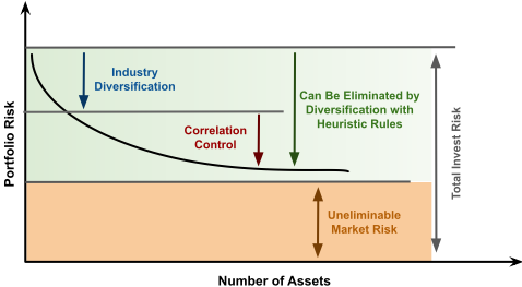
As illustrated in Figure 1, effective risk management distinguishes between reducible factors (e.g., asset selection, industry spread, and correlation control) and irreducible ones. Modern portfolio theory establishes that the reduction of unsystematic risk follows from the following equation:
where σ2 p denotes the total portfolio variance, N represents the number of constituent assets, σ2 indicates the average idiosyncratic variance (i.e., asset-specific risks), ρ signifies the mean correlation coefficient between assets, and σ2 denotes the systematic market variance. As such, the first term 1N σ2 quantifies the reducible idiosyncratic risk that diminishes with increasing asset quantity. Consequently, we can see that (1) a higher number of assets dilutes idiosyncratic risk, (2) industry diversification mitigates sector-specific volatility [Ang et al., 2009], and (3) low asset correlation amplifies diversification efficacy [Choueifaty and Coignard, 2008], isolating non-systematic risk for reduction.
Traditional reinforcement learning (RL) approaches, while adaptive to market dynamics, suffer from three critical limitations in financial applications. First, their manual reward engineering often fails to capture essential market patterns, such as momentum effects [Jegadeesh and Titman, 1993] and regime-dependent correlations [Longin and Solnik, 2001]. Second, standard RL architectures struggle to meet the requirements for sector diversification [Roncalli, 2013]. Third, their fully-connected networks do not adequately model market microstructure relationships [Aste et al., 2010]. These limitations often lead to unstable performance during black swan events [Taleb, 2010], as evidenced by the 2020 COVID19 market crash [Baker, 2020]. To address these gaps, we propose a heuristic-guided inverse reinforcement learning (IRL) framework for portfolio optimization, with the following three main components.
- The optimization module formalizes domain knowledge (sector weight caps and momentum-correlation control from [Moskowitz et al., 2012]) into synthetic expert trajectories. This overcomes data scarcity in conventional IRL methods [Ng and Russell, 2000] while maintaining financial logic consistency [Buehler et al., 2019].
- The multi-objective reward learning mechanism dynamically balances four competing objectives, namely return maximization, sector diversification [Koumou, 2020], momentum alignment [Geczy and Samonov, 2016], and correlation penalization [Buraschi et al., 2010]. The adaptive weight adjustment mechanism enables automatic rebalancing during shifts in market regimes.
- The graph-based policy network advances prior financial models through three structural innovations: explicit encoding of sector affiliation graphs, correlation graphs derived from tail dependence coefficients, and hierarchical attention mechanisms combining local asset features with asset indicators. This design enhances microstructure modeling while improving generalization ability through adaptive information fusion.
Extensive experiments and case studies on real-world financial market data demonstrate that our framework consistently outperforms several state-of-the-art baselines in terms of risk-return trade-offs and robustness to extreme events, offering a novel technical pathway for adaptive portfolio management.
2 RelatedWork
Portfolio optimization has evolved through three research paradigms. The foundational work of Markowitz [1952] established mean-variance optimization but suffered from static assumptions and sensitivity to estimation errors [Choueifaty et al., 2013]. Subsequently, some dynamic extensions, such as stochastic portfolio theory [Fernholz and Karatzas, 2005], improved market adaptability but grappled with the curse of dimensionality in multi-asset scenarios. Then, reinforcement learning (RL) emerged as a promising alternative for dynamic portfolio management. Pioneering work by Moody et al. [1998] demonstrated the potential of RL in financial time series prediction. At the same time, recent deep RL approaches [Deng et al., 2016] achieved superior risk-adjusted returns through neural policy networks. However, these methods are critically dependent on manually designed reward functions that oversimplify market complexity, a limitation extensively documented by Hambly et al. [2023] in their survey on RL-based trading systems. Inverse RL (IRL) attempted to address reward engineering challenges by learning
Algorithm 1 Greedy Expert Strategy Generation
Input: Historical returns rt, industry relation matrix I, correlation matrix C, total number of stocks N, number of stocks to select K Parameter: max industry ratio α ∈ (0, 1), threshold γ ∈ (0, 1) Output: Expert action vector at 1: Ranking all stocks based on rt in descending order as C 2: Calculate K′ ← ⌊αK⌋ 3: Initialize at ← 0 ∈ {0, 1}N and S ← ∅ 4: while |S| < K and C ̸= ∅ do 5: i ← C.pop 6: Ii ← {j | I[i, j] > 0} ∪ {i} 7: ki ← ∑j∈Ii at[j] 8: if ki ≥K′ then 9: continue 10: if S ̸= ∅ then 11: ρi ← 1 |S| ∑j∈S C[i, j] 12: if ρi ≥ γ then 13: continue 14: at[i] ← 1 and S.add(i) 15: return at
implicit objectives from expert demonstrations. The foundational IRL framework [Ng and Russell, 2000] has inspired financial applications to systematically incorporate domain knowledge through heuristic-guided reward learning.
Recently, graph-based approaches have demonstrated potential in modeling market structures. In [Chen et al., 2018], graph neural networks are employed to capture stock correlations, while temporal graphs are integrated for financial time series prediction in [Xiang et al., 2022]. Some pioneering works [Wang et al., 2019; Wang et al., 2021] utilized graph neural networks as the RL decision model to enhance the understanding of cross-asset interdependencies in portfolio management. Our heterogeneous graph attention mechanism advances these works by explicitly modeling sector hierarchies and correlation dependencies in a unified architecture, which is particularly crucial for handling cross-market portfolio optimization. The incorporation of financial domain knowledge into adaptive learning mechanisms is based on hybrid approaches such as those in [Xiong et al., 2018; Liu et al., 2021] but significantly extends these paradigms through the systematic integration of interpretable heuristics, multi-objective reward optimization, and structured market graph representation learning.
3 Methodology
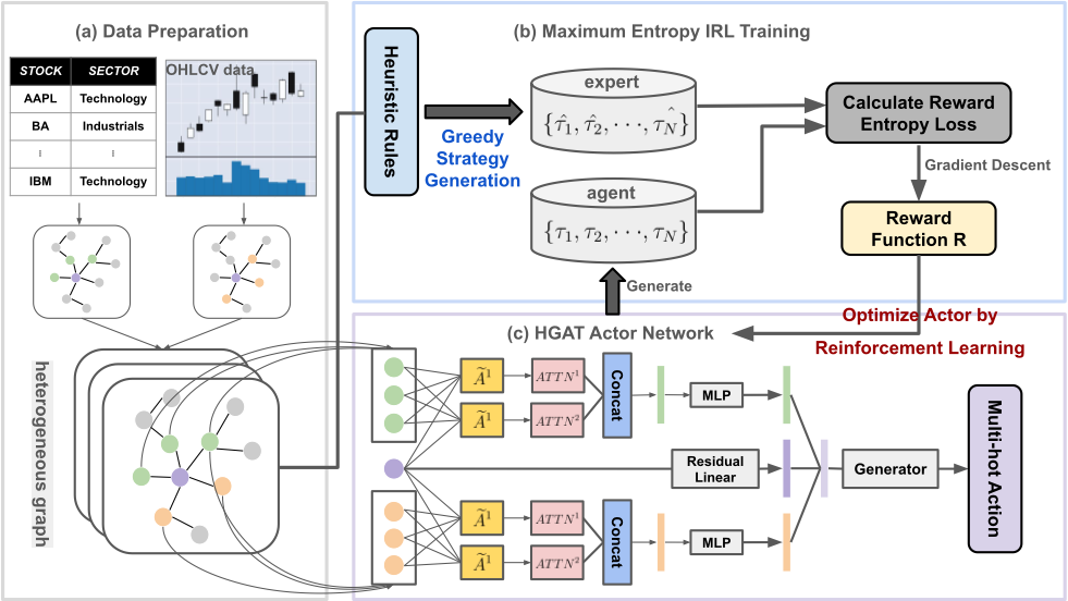
In this section, we present our proposed framework in detail. The architecture of the framework is illustrated in Figure 2.
3.1 Greedy Expert Strategy Generation with Heuristic Rules
We utilize a greedy algorithm to generate high-quality portfolio trajectories through iterative stock selection, where sector diversification and correlation constraints are incorporated. The detailed expert strategy generation procedure is described in Algorithm 1.
The process begins with ranking stocks based on their historical returns in descending order, ensuring that the most promising stocks are considered first. To manage the risk of sector concentration, we impose sector diversification constraints, limiting the maximum ratio per industry cluster to α ∈ (0, 1). That is, the number of selected stocks in each industry sector cannot exceed ⌊αK⌋, where K is the total number of stocks to select. Additionally, the strategy dynamically excludes candidates with an excessive correlation with selected stocks. If the average correlation of the stock i with the selected set S of stocks exceeds a threshold γ, given by 1 |S| ∑j∈S ρij ≥ γ, the stock will be excluded from consideration. Finally, the expert strategy outputs a binary action vector at ∈ {0, 1}N , indicating which stocks are selected for the portfolio.
3.2 Multi-Objective Reward Learning
The multi-objective reward learning component enhances the strategy by integrating four objectives: maximizing returns, diversifying across sectors, penalizing positive correlations, and incentivizing negative correlations.
Return Maximization
The return reward is based on the portfolio log-return, which is calculated as:
Sector Diversification
To promote diversification, the reward function maximizes the entropy of sector weights, defined as
Correlation Management
The positive correlation penalty discourages positive correlations among low-momentum assets, given by:
Conversely, the negative correlation incentive promotes negative correlations with high-momentum assets, represented as:
Adaptive Reward Function
The composite reward is a weighted sum of these components
with weights λi dynamically adjusted via Lagrangian duality.
3.3 MaximumEntropy Inverse Reinforcement Learning
The Maximum Entropy Inverse Reinforcement Learning (i.e., MaxEntIRL) framework, originally proposed in [Ziebart et al., 2008], addresses the ambiguity problem in estimating the reward function by preferring the reward function that maximizes entropy over the demonstrated trajectories. Our implementation extends this principle to portfolio optimization, adapting the formulation to handle non-stationary market conditions and partial observability.
Expert-Agent Reward Gap
We model the expert-agent reward loss function as:
which encourages it to learn from the expert's behavior.
We model the likelihood of expert trajectories τE under the learned reward function Rθ as:
This leads to the negative log-likelihood loss function:
where the first term encourages high rewards for expert trajectories, while the second term penalizes arbitrary scaling of rewards for agent trajectories πA, as discussed in [Finn et al., 2016]. The gradient of this loss with respect to reward parameters θ becomes
This formulation ensures that the agent policy πA covers the expert's behavior distribution while maintaining maximum entropy, crucial for handling the stochastic nature of financial markets.
Reward Network Optimization
The reward network implements a modular architecture that dynamically combines multiple financial factors through parameterized weighting. Formally, the network processes state-action pairs (st, at) through parallel encoder streams as follows:
where K = {base, ind, pos, neg} denotes the active feature modalities, ⊕ represents feature-action concatenation, and βk are learnable weights with ∑ βk = 1 through softmax normalization. The reward network parameters θ are updated via gradient clipping:
Policy Optimization
The agent policy πA is then trained using Proximal Policy Optimization (PPO) to maximize cumulative rewards under the updated reward function:
3.4 Graph-Based Policy Network
Finally, the graph-based policy learning component leverages a heterogeneous graph attention network (HGAT) to dynamically model industry relations and correlations among stocks.
Graph Construction
The industry graph Aind ∈ RN×N is constructed so that Aind,ij = 1 if stocks i and j belong to the same sector and 0 otherwise. The positive correlation graph Apos ∈ RN×N is defined as Apos,ij = 1 if correlation ρij > ρthreshold, and 0 otherwise. The correlation values are discretized as:
Multi-Head Graph Attention Encoding
Multi-head graph attention encoding is applied to the input features X ∈ RN×d , computing the attention embeddings for each graph g as H(l) g = MH-GAT(X,Ag), where the attention mechanism is calculated as:
where Q,K,V are linear transformations of the input features, and d is the feature dimension.
Heterogeneous Fusion Attention
The heterogeneous fusion attention stage concatenates the multi-head output Hind,Hpos,Hneg with raw features, calculated as:
where βk are adaptively learned weights:
Policy Generation
The fused embeddings are then fed into a generator to output normalized portfolio weights as:
where Wg is a fully-connected layer and Flatten(·) denotes the vectorization operation.
4 Experiments
In this section, we present our experimental setup and results.
4.1 Experimental Setup
To evaluate the performance of our method, we conduct extensive experiments on real-world data across the Chinese and US markets. Specifically, our evaluation is performed on the constituent stocks of the CSI 300, CSI 500, NASDAQ 100, and S&P 500 indices, covering the period from January 2018 to December 2024. Each dataset is partitioned into three subsets: a training set (from 2018 to 2022), a validation set (2023), and a test set (2024). About 5% of the stocks were discarded due to incomplete data. Raw financial data includes daily open, close, high, low, previous close prices, and trading volume. These features are normalized using rolling-window standardization (the window size is set to 20 days) and further grouped via k-means clustering for intra-group normalization. Monthly correlation matrices are computed using Pearson's correlation coefficients, with positive correlation graphs (edges for ρij > 0.2) and negative correlation graphs (edges for ρij < -0.2) generated to capture dynamic market interactions.
We compare our method with state-of-the-art deep learning (DL) models (including LSTM [Hochreiter and Schmidhuber, 1997], GRU [Chung et al., 2014], ALSTM [Feng et al., 2019], Transformer [Vaswani et al., 2017], PatchTST [Nie et al., 2023], DLinear [Zeng et al., 2023], iTransformer [Liu et al., 2024], Crossformer [Zhang and Yan, 2023], and MASTER [Li et al., 2024]), reinforcement learning (RL) models (including AlphaStock [Wang et al., 2019], DeepTrader [Wang et al., 2021], and DeepPocket [Soleymani and Paquet, 2021]), and large language model (LLM) models for time series (including GPT4TS [Zhou et al., 2023], TIME-LLM [Jin et al., 2024], and aLLM4TS [Bian et al., 2024]).
We use the following six metrics for performance evaluation: Annualized Return Rate (ARR), Annualized Volatility (AVol), Maximum Drawdown (MDD), Sharpe Ratio (SR), Calmar Ratio (CR), and Information Ratio (IR). To eliminate fluctuations, we average the metrics over three repeated tests for each model. Hyperparameters are configured with a learning rate of 10-4 , a batch size of 128, and HGAT policy networks featuring 128-dimensional hidden layers, 8 attention heads, and 200 training epochs.
Correlation matrices and graph structures are generated monthly, producing industry relation graphs (Aind), positive correlation graphs (Apos) and negative correlation graphs (Aneg). Synthetic expert trajectories are created to enforce sector diversification constraints and correlation control rules. We construct training and prediction datasets by encapsulating time-series features, graph structures, and labels into PyTorch Geometric Data objects. The IRL training loop initializes a multi-objective reward network and an HGAT policy network, alternately optimizing the reward function via MaxEntIRL and the actor-critic policy via Stable-Baselines3 PPO.
4.2 Performance Analysis
The overall results of all methods across four datasets are presented in Table 1. These results demonstrate the superior performance of our proposed method in different scenarios. Our method consistently outperforms the state-of-theart baseline models in terms of key return metrics, especially ARR, SR, and CR. In addition to superior returns, our method also demonstrates competitive performance in terms of risk metrics such as AVol and MDD. On the CSI 300 dataset, our method significantly outperforms the baseline methods with an ARR of 0.491, surpassing the closest competitor (iTransformer: 0.372) by 31.9%. This superiority extends to riskadjusted returns, as evidenced by the highest SR (1.777) and CR (5.134), indicating enhanced returns per unit of risk and drawdown. In particular, while our method exhibits moderate volatility (AVol: 0.225), its MDD (-0.095) remains competitive, slightly under-performing ALSTM (-0.073) but demonstrating improved resilience compared to other models. On the NASDAQ 100 dataset, our method achieves the highest ARR (0.432), outperforming Transformer (0.258) by substantial margins. However, its IR (0.433) lags behind other models, suggesting potential opportunities to refine risk-adjusted performance in highly volatile markets. On the CSI 500 dataset, our method achieves a remarkable Annualized Return Rate (ARR) of 0.710, outperforming all baseline models by a significant margin (+36.8% over GPT4TS: 0.519 and +28.1% over TIME-LLM: 0.554). This superior return generation is complemented by competitive risk management, as evidenced by an Annualized Volatility (AVol) of 0.290, which is lower than most models, except DeepPocket (0.260). While the MDD (-0.161) is slightly higher than PatchTST's (-0.129), our method demonstrates exceptional risk-adjusted performance with the highest Sharpe Ratio (SR: 1.847) and Calmar Ratio (CR: 4.406), indicating superior returns per unit of risk and drawdown. However, the Information Ratio (IR: 1.058) trails TIME-LLM (1.470), suggesting potential enhancements in aligning returns with benchmark consistency. For the S&P 500 dataset, our method achieves an ARR of 0.250, which, although lower than GPT4TS (0.321), is accompanied by the lowest AVol (0.117) and a competitive MDD (-0.058), outperforming even DeepTrader (-0.049) when normalized against return metrics. Its SR (1.906) and CR (4.293) rank second only to GPT4TS (2.034 and 4.346), highlighting a robust risk-return trade-off. In particular, the model's IR (1.184) remains moderate compared to GPT4TS (1.872), indicating room for improvement in benchmarkrelative efficiency. Comparative analysis reveals distinct strengths across models. GPT4TS dominates absolute returns on the S&P 500 dataset but exhibits higher volatility (AVol: 0.157), while DeepTrader achieves the lowest MDD (-0.049) at the cost of suboptimal returns. PatchTST excels in minimizing drawdowns on the CSI 500 dataset (-0.129) but lags in ARR. Our method's hybrid architecture-likely integrating temporal feature extraction with dynamic risk mitigationenables balanced performance, prioritizing high returns and stability.
In summary, our method establishes state-of-the-art performance on the CSI 300, NASDAQ 100, and CSI 500 datasets and delivers competitive, low-volatility results on the S&P 500 dataset, indicating that it effectively leads to more robust and adaptive portfolio management.
4.3 Ablation Study
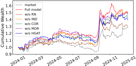
To validate the effectiveness of key components in our proposed model, we perform an ablation study by sequentially removing specific modules while keeping other modules and parameters unchanged. The quantitative results are shown in Table 2, which are further supplemented by cumulative return curves in Figure 3.
The quantitative results and cumulative return curves confirm the following findings. The full model maintains superior risk-adjusted growth with smoother equity trajectories, while ablated variants exhibit either lower terminal returns or higher volatility. They collectively demonstrate that each proposed component makes a unique contribution to the model's robustness and profitability.
| Model | CSI 300 | NASDAQ 100 | ||||||||||
|---|---|---|---|---|---|---|---|---|---|---|---|---|
| ARR | AVol | MDD | SR | CR | IR | ARR | AVol | MDD | SR | CR | IR | |
| LSTM | 0.104 | 0.243 | -0.173 | 0.431 | 0.605 | 0.536 | 0.140 | 0.165 | -0.095 | 0.8522 | 1.470 | 0.883 |
| GRU | 0.166 | 0.234 | -0.154 | 0.707 | 1.076 | 0.779 | 0.229 | 0.239 | -0.148 | 0.957 | 1.542 | 1.088 |
| ALSTM | 0.287 | 0.198 | -0.073 | 1.444 | 3.904 | 1.442 | 0.235 | 0.256 | -0.172 | 0.918 | 1.370 | 1.070 |
| Transformer | 0.235 | 0.221 | -0.158 | 1.065 | 1.492 | 1.112 | 0.258 | 0.271 | -0.221 | 0.951 | 1.167 | 1.074 |
| PatchTST | 0.308 | 0.243 | -0.141 | 1.265 | 2.174 | 1.213 | 0.206 | 0.173 | -0.112 | 1.190 | 1.844 | 1.279 |
| DLinear | 0.192 | 0.287 | -0.143 | 0.669 | 1.341 | 0.816 | 0.081 | 0.222 | -0.181 | 0.362 | 0.444 | 0.489 |
| iTransformer | 0.372 | 0.309 | -0.148 | 1.203 | 2.498 | 1.184 | 0.088 | 0.253 | -0.163 | 0.349 | 0.544 | 0.590 |
| Crossformer | 0.359 | 0.234 | -0.157 | 1.532 | 2.280 | 1.520 | 0.192 | 0.231 | -0.128 | 0.831 | 1.498 | 0.944 |
| MASTER | 0.194 | 0.223 | -0.107 | 0.869 | 1.816 | 0.960 | 0.229 | 0.194 | -0.151 | 1.180 | 1.515 | 1.219 |
| AlphaStock | 0.308 | 0.215 | -0.105 | 1.431 | 2.924 | 1.360 | 0.131 | 0.172 | -0.123 | 0.759 | 1.065 | 0.803 |
| DeepTrader | 0.385 | 0.293 | -0.162 | 1.313 | 2.377 | 1.323 | 0.183 | 0.196 | -0.108 | 0.924 | 1.698 | 1.161 |
| DeepPocket | 0.207 | 0.203 | -0.135 | 1.016 | 1.528 | 1.029 | 0.106 | 0.145 | -0.097 | 0.732 | 1.099 | 0.771 |
| GPT4TS | 0.333 | 0.330 | -0.198 | 1.009 | 1.682 | 1.103 | 0.242 | 0.221 | -0.077 | 1.093 | 3.116 | 1.104 |
| TIME-LLM | 0.370 | 0.323 | -0.209 | 1.145 | 1.771 | 1.205 | 0.183 | 0.246 | -0.139 | 0.745 | 1.320 | 0.896 |
| aLLM4TS | 0.312 | 0.331 | -0.177 | 0.943 | 1.764 | 1.057 | 0.183 | 0.210 | -0.119 | 0.869 | 1.538 | 0.879 |
| (* Ours) | 0.491 | 0.225 | -0.095 | 1.777 | 5.134 | 0.381 | 0.432 | 0.182 | -0.125 | 1.978 | 3.449 | 0.433 |
| Model | CSI 500 | S&P 500 | ||||||||||
| ARR | AVol | MDD | SR | CR | IR | ARR | AVol | MDD | SR | CR | IR | |
| LSTM | 0.161 | 0.313 | -0.199 | 0.514 | 0.808 | 0.656 | 0.183 | 0.126 | -0.070 | 1.450 | 2.611 | 1.416 |
| GRU | 0.135 | 0.292 | -0.199 | 0.461 | 0.677 | 0.565 | 0.204 | 0.131 | -0.075 | 1.558 | 2.697 | 1.456 |
| ALSTM | 0.240 | 0.310 | -0.279 | 0.775 | 0.861 | 0.866 | 0.236 | 0.151 | -0.103 | 1.556 | 2.281 | 1.546 |
| Transformer | 0.193 | 0.306 | -0.228 | 0.629 | 0.845 | 0.695 | 0.244 | 0.145 | -0.102 | 1.682 | 2.376 | 1.630 |
| PatchTST | 0.245 | 0.281 | -0.129 | 0.872 | 1.903 | 0.875 | 0.176 | 0.166 | -0.087 | 1.063 | 2.024 | 1.089 |
| DLinear | 0.347 | 0.336 | -0.174 | 1.033 | 1.987 | 1.070 | 0.167 | 0.150 | -0.085 | 1.111 | 1.952 | 1.095 |
| iTransformer | 0.218 | 0.329 | -0.149 | 0.662 | 1.461 | 0.748 | 0.082 | 0.156 | -0.095 | 0.523 | 0.860 | 0.644 |
| Crossformer | 0.307 | 0.296 | -0.187 | 1.034 | 1.635 | 1.016 | 0.228 | 0.141 | -0.088 | 1.613 | 2.600 | 1.537 |
| MASTER | 0.413 | 0.333 | -0.205 | 1.241 | 2.013 | 1.201 | 0.150 | 0.147 | -0.079 | 1.014 | 1.896 | 1.032 |
| AlphaStock | 0.051 | 0.273 | -0.172 | 0.187 | 0.297 | 0.318 | 0.148 | 0.118 | -0.057 | 1.257 | 2.584 | 1.236 |
| DeepTrader | 0.273 | 0.331 | -0.155 | 0.825 | 1.759 | 1.002 | 0.171 | 0.118 | -0.049 | 1.457 | 3.467 | 1.460 |
| DeepPocket | 0.141 | 0.260 | -0.174 | 0.809 | 0.637 | 0.116 | -0.065 | 1.156 | 2.056 | 1.147 | ||
| GPT4TS | 0.519 | 0.344 | -0.200 | 0.541 | 2.590 | 1.378 | 0.134 0.321 | 0.157 | -0.073 | 2.034 | 4.346 | |
| TIME-LLM | 0.554 | 0.342 | 1.510 | 2.699 | 1.470 | 0.240 | -0.155 | 0.543 | 0.842 | 1.872 | ||
| 0.376 | -0.205 | 1.617 | 1.523 | 1.115 | 0.130 | -0.083 | 1.481 | 2.821 | 0.682 1.396 | |||
| aLLM4TS | 0.337 | -0.247 | 1.115 | 0.236 | 0.159 | |||||||
| (* Ours) | 0.710 | 0.290 | -0.161 | 1.847 | 4.406 | 1.058 | 0.250 | 0.117 | -0.058 | 1.906 | 4.293 | 1.184 |
Necessity of Reward Network (RN) Learning
Removing the dedicated reward network and directly using portfolio returns severely degrades the performance of the framework. The 38.9% decrease in the Annualized Return Rate (ARR) and 34.4% reduction in the Sharpe Ratio (SR) demonstrate the critical role of RN. This aligns with our conjecture that the handcrafted reward mechanism better captures nonlinear market dynamics than raw returns.
Effectiveness of Industry Diversification
Although removing industry constraints can slightly improve ARR (+2.7%), it causes significantly deeper drawdowns (- 15.0% vs. -10.1%) and lower CR. This indicates a risk-return trade-off: Industry concentration may boost short-term returns but increases portfolio volatility, which justifies the role of diversification constraints in our framework.
Effectiveness of Correlation Management
The 12.9% reduction of ARR and SR when turning off correlation control highlights its importance in stabilizing returns. This module appears particularly effective in avoiding simultaneous drawdowns of highly correlated assets.
| Model | Component Configuration | ARR | SR | MDD | CR |
|---|---|---|---|---|---|
| Full Model | Our proposed model with all modules | 0.554 | 1.923 | -0.101 | 5.473 |
| w/o RN | Replace reward network with portfolio return | 0.338 | 1.261 | -0.113 | 2.986 |
| w/o MOR | Remove multi-objective reward module | 0.536 | 1.868 | -0.142 | 3.757 |
| w/o InD | Remove industry diversification constraints | 0.569 | 1.938 | -0.150 | 3.781 |
| w/o COR | Remove correlation control | 0.482 | 1.674 | -0.115 | 4.165 |
| w/o HGAT | Replace HGAT policy network with MLP | 0.448 | 1.666 | -0.101 | 4.415 |
Effectiveness of Heterogeneous Graph Attention Network (HGAT)
Replacing the HGAT with MLP degrades all evaluation metrics, particularly with ARR decreasing by 19.1%. This validates our design choice to leverage graph-structured market data through attention mechanisms, capturing complex asset relationships.
4.4 Case Study: Market Regime Analysis
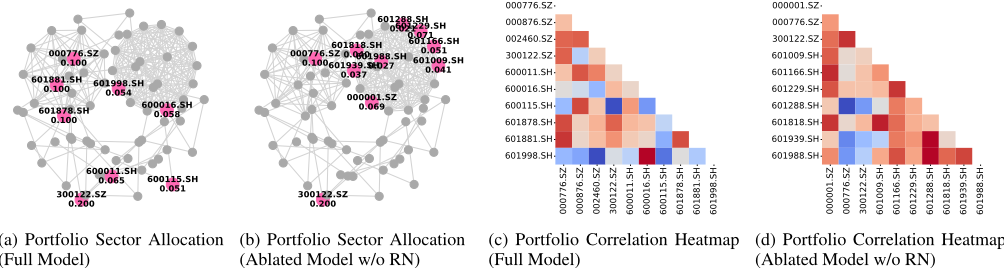
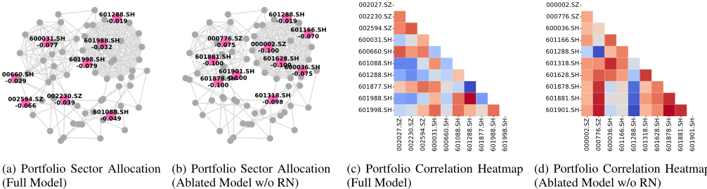
To validate the role of heuristic rules in our framework, we present regime-specific case studies by visualizing the portfolio sector distributions and stock correlation heatmaps (where darker red indicates stronger positive correlation and darker blue indicates stronger negative correlation) across two contrasting market conditions in Figures 4 (bull market: 2024.9) and 5 (bear market: 2024.10). These visualized results reveal the fundamental behavioral patterns in our framework. The portfolio provided by the full model shows balanced exposure across defensive/cyclical sectors in both market regimes, while the ablated model exhibits excessive concentration in dominant sectors. In the bull market dynamic, the full model prioritizes momentum continuation through sustained exposure to growth sectors. While in a bear market dynamic, it activates mean-reversion patterns by shifting to undervalued (negative-related) assets, whereas the ablated model maintains momentum-chasing in declines. These heuristic rules for adaptation enable dynamic balancing between maximizing returns and containing risk across market cycles.
5 Conclusion
This paper proposes a novel heuristic-guided inverse reinforcement learning (IRL) framework for portfolio optimization that effectively integrates financial domain expertise with advanced AI techniques. Our experimental results demonstrate that our proposed framework achieves significant improvements in performance and versatility across both Chinese and US markets, enhancing Sharpe and Calmar ratios considerably compared to existing DL, RL, and LLM-based methods and exhibiting robustness through controlled drawdowns during periods of market volatility. These promising results suggest the potential of our framework to bridge traditional portfolio management with modern AI techniques, thereby contributing to the development of more effective investment strategies in an increasingly complex financial landscape. Future work will explore further the applications of our framework in real-world trading scenarios.
Acknowledgements
This work was supported in part by the National Natural Science Foundation of China under Grant Number 62202169 and the Shanghai Sailing Program 23YF1410600.
@inproceedings{ijcai2025p1054,
  title     = {Enhancing Portfolio Optimization via Heuristic-Guided Inverse Reinforcement Learning with Multi-Objective Reward and Graph-based Policy Learning},
  author    = {Zhang, Wenyi and Jia, Renjun and Wang, Yanhao and Cheng, Dawei and Zhao, Minghao and Chen, Cen},
  booktitle = {Proceedings of the Thirty-Fourth International Joint Conference on
               Artificial Intelligence, {IJCAI-25}},
  publisher = {International Joint Conferences on Artificial Intelligence Organization},
  editor    = {James Kwok},
  pages     = {9483--9491},
  year      = {2025},
  month     = {8},
  note      = {AI4Tech: AI Enabling Technologies},
  doi       = {10.24963/ijcai.2025/1054},
  url       = {https://doi.org/10.24963/ijcai.2025/1054},
}
TY - CPAPER TI - Enhancing Portfolio Optimization via Heuristic-Guided Inverse Reinforcement Learning with Multi-Objective Reward and Graph-based Policy Learning AU - Zhang, Wenyi AU - Jia, Renjun AU - Wang, Yanhao AU - Cheng, Dawei AU - Zhao, Minghao AU - Chen, Cen T2 - Proceedings of the Thirty-Fourth International Joint Conference on Artificial Intelligence, IJCAI-25 PB - International Joint Conferences on Artificial Intelligence Organization PY - 2025 SP - 9483 EP - 9491 DO - 10.24963/ijcai.2025/1054 UR - https://doi.org/10.24963/ijcai.2025/1054 ER -Copied
Machine-readable versions of this paper, for tools and AI agents:





