
Concentrate on Weakness: Mining Hard Prototypes for Few-Shot Medical Image Segmentation
Proceedings of the Thirty-Fourth International Joint Conference on Artificial Intelligence. Main Track. Pages 1242-1250.
https://doi.org/10.24963/ijcai.2025/139
Keywords
- Computer Vision: CV: Biomedical image analysis
- Computer Vision: CV: Segmentation, grouping and shape analysis
- Computer Vision: CV: Transfer, low-shot, semi- and un- supervised learning
- Computer Vision: CV: Machine learning for vision
Abstract
Few-Shot Medical Image Segmentation (FSMIS) has been widely used to train a model that can perform segmentation from only a few annotated images. However, most existing prototype-based FSMIS methods generate multiple prototypes from the support image solely by random sampling or local averaging, which can cause particularly severe boundary blurring due to the tendency for normal features accounting for the majority of features of a specific category. Consequently, we propose to focus more attention to those weaker features that are crucial for clear segmentation boundary. Specifically, we design a Support Self-Prediction (SSP) module to identify such weak features by comparing true support mask with one predicted by global support prototype. Then, a Hard Prototypes Generation (HPG) module is employed to generate multiple hard prototypes based on these weak features. Subsequently, a Multiple Similarity Maps Fusion (MSMF) module is devised to generate final segmenting mask in a dual-path fashion to mitigate the imbalance between foreground and background in medical images. Furthermore, we introduce a boundary loss to further constraint the edge of segmentation. Extensive experiments on three publicly available medical image datasets demonstrate that our method achieves state-of-the-art performance. Code is available at https://github.com/jcjiang99/CoW.
- [Cao et al., 2022] Hu Cao, Yueyue Wang, Joy Chen, Dong- sheng Jiang, Xiaopeng Zhang, Qi Tian, and Manning Wang. Swin-unet: Unet-like pure transformer for medi- cal image segmentation. In ECCV, pages 205-218, 2022.
- [Chen et al., 2018] Liang Chen, Paul Bentley, Kensaku Mori, Kazunari Misawa, Michitaka Fujiwara, and Daniel Rueckert. Drinet for medical image segmentation. IEEE Transactions on Medical Imaging, 37(11):2453-2462, 2018.
- [Chen et al., 2021] Xuming Chen, Shanlin Sun, Narisu Bai, Kun Han, Qianqian Liu, Shengyu Yao, Hao Tang, Chu- peng Zhang, Zhipeng Lu, Qian Huang, et al. A deep learning-based auto-segmentation system for organs-at- risk on whole-body computed tomography images for ra- diation therapy. Radiotherapy and Oncology, 160:175- 184, 2021.
- [Cheng et al., 2024] Ziming Cheng, Shidong Wang, Tong Xin, Tao Zhou, Haofeng Zhang, and Ling Shao. Few- shot medical image segmentation via generating multiple representative descriptors. IEEE Transactions on Medical Imaging, 2024.
- [Dolz et al., 2018] Jose Dolz, Karthik Gopinath, Jing Yuan, Herve Lombaert, Christian Desrosiers, and Ismail Ben Ayed. Hyperdense-net: a hyper-densely connected cnn for multi-modal image segmentation. IEEE Transactions on Medical Imaging, 38(5):1116-1126, 2018.
- [Dong and Xing, 2018] Nanqing Dong and Eric P Xing. Few-shot semantic segmentation with prototype learning. In BMVC, pages 1-11, 2018.
- [El Naqa et al., 2007] Issam El Naqa, Deshan Yang, Aditya Apte, Divya Khullar, Sasa Mutic, Jie Zheng, Jeffrey D Bradley, Perry Grigsby, and Joseph O Deasy. Concur- rent multimodality image segmentation by active contours for radiotherapy treatment planning a. Medical physics, 34(12):4738-4749, 2007.
- [Fang and Yan, 2020] Xi Fang and Pingkun Yan. Multi- organ segmentation over partially labeled datasets with multi-scale feature abstraction. IEEE Transactions on Medical Imaging, 39(11):3619-3629, 2020.
- [Finn et al., 2017] Chelsea Finn, Pieter Abbeel, and Sergey Levine. Model-agnostic meta-learning for fast adaptation of deep networks. In ICML, pages 1126-1135, 2017.
- [Garcia and Bruna, 2017] Victor Garcia and Joan Bruna. Few-shot learning with graph neural networks. arXiv preprint arXiv:1711.04043, 2017.
- [Gu et al., 2020] Ran Gu, Guotai Wang, Tao Song, Rui Huang, Michael Aertsen, Jan Deprest, Sébastien Ourselin, Tom Vercauteren, and Shaoting Zhang. Ca-net: Com- prehensive attention convolutional neural networks for ex- plainable medical image segmentation. IEEE Transactions on Medical Imaging, 40(2):699-711, 2020.
- [Hansen et al., 2022] Stine Hansen, Srishti Gautam, Robert Jenssen, and Michael Kampffmeyer. Anomaly detection- inspired few-shot medical image segmentation through self-supervision with supervoxels. Medical Image Anal- ysis, 78:102385, 2022.
- [Hartigan and Wong, 1979] John A Hartigan and Manchek A Wong. Algorithm as 136: A k-means clustering algorithm. Journal of the Royal Statistical Society. Series C (Applied Statistics), 28(1):100-108, 1979.
- [Hesamian et al., 2019] Mohammad Hesam Hesamian, Wenjing Jia, Xiangjian He, and Paul Kennedy. Deep learning techniques for medical image segmentation: achievements and challenges. Journal of Digital Imaging, 32:582-596, 2019.
- [Isensee et al., 2021] Fabian Isensee, Paul F Jaeger, Si- mon AA Kohl, Jens Petersen, and Klaus H Maier-Hein. nnu-net: a self-configuring method for deep learning- based biomedical image segmentation. Nature methods, 18(2):203-211, 2021.
- [Kavur et al., 2021] A Emre Kavur, N Sinem Gezer, Mustafa Barıs ¸, Sinem Aslan, Pierre-Henri Conze, Vladimir Groza, Duc Duy Pham, Soumick Chatterjee, Philipp Ernst, Savas ¸ Özkan, et al. Chaos challenge-combined (ct-mr) healthy abdominal organ segmentation. Medical Image Analysis, 69:101950, 2021.
- [Landman et al., 2015] Bennett Landman, Zhoubing Xu, J Igelsias, Martin Styner, Thomas Langerak, and Arno Klein. Miccai multi-atlas labeling beyond the cranial vault-workshop and challenge. In MICCAI Workshop Challenge, volume 5, page 12, 2015.
- [Li et al., 2018] Xiaomeng Li, Hao Chen, Xiaojuan Qi, Qi Dou, Chi-Wing Fu, and Pheng-Ann Heng. H- denseunet: hybrid densely connected unet for liver and tu- mor segmentation from ct volumes. IEEE Transactions on Medical Imaging, 37(12):2663-2674, 2018.
- [Lin et al., 2014] Tsung-Yi Lin, Michael Maire, Serge Be- longie, James Hays, Pietro Perona, Deva Ramanan, Piotr Dollár, and C Lawrence Zitnick. Microsoft coco: Com- mon objects in context. In ECCV, pages 740-755, 2014.
- [Lin et al., 2023] Yi Lin, Yufan Chen, Kwang-Ting Cheng, and Hao Chen. Few shot medical image segmentation with cross attention transformer. In MICCAI, pages 233-243, 2023.
- [Long et al., 2015] Jonathan Long, Evan Shelhamer, and Trevor Darrell. Fully convolutional networks for seman- tic segmentation. In CVPR, pages 3431-3440, 2015.
- [Luo et al., 2021] Xiangde Luo, Jieneng Chen, Tao Song, and Guotai Wang. Semi-supervised medical image seg- mentation through dual-task consistency. In AAAI, pages 8801-8809, 2021.
- [Ouyang et al., 2020] Cheng Ouyang, Carlo Biffi, Chen Chen, Turkay Kart, Huaqi Qiu, and Daniel Rueckert. Self- supervision with superpixels: Training few-shot medical image segmentation without annotation. In ECCV, pages 762-780, 2020.
- [Ouyang et al., 2022] Cheng Ouyang, Carlo Biffi, Chen Chen, Turkay Kart, Huaqi Qiu, and Daniel Rueckert. Self- supervised learning for few-shot medical image segmenta- tion. IEEE Transactions on Medical Imaging, 41(7):1837- 1848, 2022.
- [Peiris et al., 2022] Himashi Peiris, Munawar Hayat, Zhaolin Chen, Gary Egan, and Mehrtash Harandi. A robust volumetric transformer for accurate 3d tumor segmentation. In MICCAI, pages 162-172, 2022.
- [Ronneberger et al., 2015] Olaf Ronneberger, Philipp Fis- cher, and Thomas Brox. U-net: Convolutional networks for biomedical image segmentation. In MICCAI, pages 234-241, 2015.
- [Roy et al., 2020] Abhijit Guha Roy, Shayan Siddiqui, Se- bastian Pölsterl, Nassir Navab, and Christian Wachinger. 'squeeze & excite'guided few-shot segmentation of volu- metric images. Medical image analysis, 59:101587, 2020.
- [Shaban et al., 2017] Amirreza Shaban, Shray Bansal, Zhen Liu, Irfan Essa, and Byron Boots. One-shot learning for semantic segmentation. arXiv preprint arXiv:1709.03410, 2017.
- [Shen et al., 2023] Qianqian Shen, Yanan Li, Jiyong Jin, and Bin Liu. Q-net: Query-informed few-shot medical image segmentation. In Proceedings of SAI Intelligent Systems Conference, pages 610-628, 2023.
- [Shi et al., 2021] Gonglei Shi, Li Xiao, Yang Chen, and S Kevin Zhou. Marginal loss and exclusion loss for par- tially supervised multi-organ segmentation. Medical Im- age Analysis, 70:101979, 2021.
- [Snell et al., 2017] Jake Snell, Kevin Swersky, and Richard Zemel. Prototypical networks for few-shot learning. In NeurIPS, volume 30, 2017.
- [Sung et al., 2018] Flood Sung, Yongxin Yang, Li Zhang, Tao Xiang, Philip HS Torr, and Timothy M Hospedales. Learning to compare: Relation network for few-shot learn- ing. In CVPR, pages 1199-1208, 2018.
- [Tang et al., 2024] Song Tang, Shaxu Yan, Xiaozhi Qi, Jianxin Gao, Mao Ye, Jianwei Zhang, and Xiatian Zhu. Few-shot medical image segmentation with high-fidelity prototypes. Medical Image Analysis, page 103412, 2024.
- [Tsochatzidis et al., 2021] Lazaros Tsochatzidis, Panagiota Koutla, Lena Costaridou, and Ioannis Pratikakis. Integrat- ing segmentation information into cnn for breast cancer diagnosis of mammographic masses. Computer Methods and Programs in Biomedicine, 200:105913, 2021.
- [Van der Maaten and Hinton, 2008] Laurens Van der Maaten and Geoffrey Hinton. Visualizing data using t-sne. Journal of machine learning research, 9(11), 2008.
- [Vinyals et al., 2016] Oriol Vinyals, Charles Blundell, Tim- othy Lillicrap, Daan Wierstra, et al. Matching networks for one shot learning. In NeurIPS, pages 3637-364, 2016.
- [Wang et al., 2018] Guotai Wang, Maria A Zuluaga, Wenqi Li, Rosalind Pratt, Premal A Patel, Michael Aertsen, Tom Doel, Anna L David, Jan Deprest, Sébastien Ourselin, et al. Deepigeos: a deep interactive geodesic framework for medical image segmentation. IEEE Transactions on Pattern Analysis and Machine Intelligence, 41(7):1559- 1572, 2018.
- [Wang et al., 2019] Kaixin Wang, Jun Hao Liew, Yingtian Zou, Daquan Zhou, and Jiashi Feng. Panet: Few-shot im- age semantic segmentation with prototype alignment. In ICCV, pages 9197-9206, 2019.
- [Wang et al., 2022] Runze Wang, Qin Zhou, and Guoyan Zheng. Few-shot medical image segmentation regularized with self-reference and contrastive learning. In MICCAI, pages 514-523, 2022.
- [Wu et al., 2019] Yicheng Wu, Yong Xia, Yang Song, Dong- hao Zhang, Dongnan Liu, Chaoyi Zhang, and Weidong Cai. Vessel-net: Retinal vessel segmentation under multi- path supervision. In MICCAI, pages 264-272, 2019.
- [Wu et al., 2022] Huisi Wu, Fangyan Xiao, and Chongxin Liang. Dual contrastive learning with anatomical auxiliary supervision for few-shot medical image segmentation. In ECCV, pages 417-434, 2022.
- [Yang et al., 2020] Boyu Yang, Chang Liu, Bohao Li, Jian- bin Jiao, and Qixiang Ye. Prototype mixture models for few-shot semantic segmentation. In MICCAI, pages 763- 778, 2020.
- [Zaidi and El Naqa, 2010] Habib Zaidi and Issam El Naqa. Pet-guided delineation of radiation therapy treatment vol- umes: a survey of image segmentation techniques. Euro- pean Journal of Nuclear Medicine and Molecular Imag- ing, 37:2165-2187, 2010.
- [Zheng et al., 2024] Meng Zheng, Benjamin Planche, Zhongpai Gao, Terrence Chen, Richard J Radke, and Ziyan Wu. Few-shot 3d volumetric segmentation with multi-surrogate fusion. In MICCAI, pages 286-296, 2024.
- [Zhu et al., 2023] Yazhou Zhu, Shidong Wang, Tong Xin, and Haofeng Zhang. Few-shot medical image segmenta- tion via a region-enhanced prototypical transformer. In MICCAI, pages 271-280, 2023.
- [Zhuang, 2018] Xiahai Zhuang. Multivariate mixture model for myocardial segmentation combining multi-source im- ages. IEEE Transactions on Pattern Analysis and Machine Intelligence, 41(12):2933-2946, 2018.
References were extracted automatically from the PDF and may contain errors.
Full text extracted automatically from the PDF; figures, tables and equations may differ. The PDF is the version of record.
1 Introduction
Automatic segmentation of organs, tissues and lesions appearing in medical images is broadly applied in clinical research, including disease diagnosis [Tsochatzidis et al., 2021], treatment planning [El Naqa et al., 2007; Zaidi and El Naqa, 2010; Chen et al., 2021] and surgical guidance [Wang et al., 2018; Hesamian et al., 2019]. Recently, fully supervised deep learning segmentation frameworks [Fang and Yan, 2020; Shi et al., 2021; Isensee et al., 2021] exhibit superior performance, but they heavily depend on large amounts of densely annotated training data, which is impractical for medical scenarios for the reason that labeling medical images requires considerable clinical expertise, cost and time [Luo et al., 2021].
∗Corresponding author.
To solve this challenge, Few-Shot Learning (FSL) [Snell et al., 2017; Sung et al., 2018; Garcia and Bruna, 2017; Finn et al., 2017] has been proposed as a potential learning paradigm to train models that can efficiently adapt to novel classes when given extremely scarce annotated data [Shaban et al., 2017], based on which corresponding segmentation method is called Few-Shot Medical Image Segmentation (FSMIS). In particular, FSMIS typically trains models with base classes and segment unseen classes in the inference stage. Consequently, models trained in this manner are capable of segmenting novel organ or lesion leveraging solely a few annotated data, evading the need for retraining, which holds significant importance for medical image segmentation.
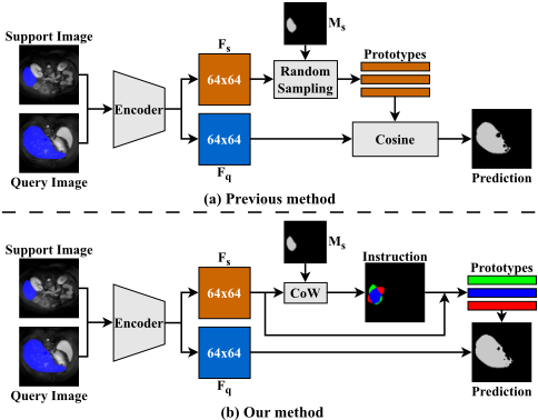
As one of dense image prediction tasks, FSMIS has an indispensable demand for features with strong category information and precise spatial boundary details. In order to leverage the annotated samples, the majority of current FSMIS models distill prior knowledge based on prototype network [Ouyang et al., 2020; Shen et al., 2023; Wu et al., 2022], among which multiple prototypes-based network is the predominant method. However, these methods generate multiple prototypes from support images either by a random selecting strategy or simple local averaging, which incline to normal features in the central area of a specific organ or involve background information in foreground prototypes as illustrated in Fig. 1(a). Furthermore, those weaker features mainly distributed along the boundary of the organ are neglected to a considerable extent, which can lead to a poorly segmentation boundary. As a result, some foreground and background points will be misclassified due to the excessive focus on normal features.
In this paper, we propose a Concentrate on Weakness (CoW) approach that learns to mine hard prototypes for each category to represent its feature distribution more comprehensively as illustrated in Fig. 1(b), to tackle the aforementioned problem. Specifically, we devise a Support Self-Prediction (SSP) module to provide knowledge for weak features carrying critical boundary information, which are subsequently utilized by the Hard Prototypes Generation (HPG) module to generate hard prototypes to improve segmentation accuracy and robustness. Right after is the Multiple Similarity Maps Fusion (MSMF) module that fuses multiple similarity maps to incorporate comprehensive information included in them to get the final predicted mask. To acquire a more precise segmenting boundary, we also devise a boundary loss, which effectively suppress over-segmentation whether for the foreground or the background. In conclusion, our main contributions are summarized as follows:
- We propose a novel method to identify weak features by comparing predicted support mask and its true label. Besides, multiple hard prototypes are generated by further processing those weak features, ensuring more comprehensive representation of overall distribution.
- To make full use of the information provided by generated multiple prototypes, we design an MSMF module to fuse multiple similarity maps predicted by these prototypes to get the final mask.
- Extensive experiments conducted on three popular medical image datasets reveal that our proposed model outperforms other existing state-of-the-art (SOTA) models and exhibits significant performance improvements.
2 RelatedWork
2.1 Medical Image Segmentation
With the development of Convolutional Neural Networks (CNNs), deep learning methods have become the dominated approach to MIS on various tumor [Peiris et al., 2022], anatomical structures [Dolz et al., 2018] and lesions [Li et al., 2018] recently. Fully Convolutional Networks (FCNs), which replace the fully connected layers of standard CNNs with fully convolutional layers, prove to be a powerful net architecture for semantic segmentation [Long et al., 2015]. Afterwards, the encoder-decoder networks gradually become the prevailing architecture for semantic segmentation, among which U-Net is a widely recognized method for MIS with remarkable results [Ronneberger et al., 2015]. Besides, most recent MIS networks are designed based on visual transformer [Cao et al., 2022], multi-scale fusion [Wu et al., 2019], feature pyramid [Chen et al., 2018] and self-attention mechanism [Gu et al., 2020]. Unfortunately, all these models require abundant densely annotated data.
2.2 Few-Shot Medical Image Segmentation
FSMIS is a promising approach since it can work with a few labeled samples. The prototypical network [Wang et al., 2019; Ouyang et al., 2020], which extracts representative prototypes of semantic classes from the support, is one of prevalent FSMIS methods featured by its strong interpretability. PANet [Wang et al., 2019] argues that parametric segmentation generalizes poorly and proposes a non-parametric prototype matching method with a prototype alignment regularization. ADNet [Hansen et al., 2022] builds further on the branch initiated by PANet [Wang et al., 2019] and does not explicitly model the complex background class namely relying solely on one foreground prototype. Q-Net [Shen et al., 2023] replaces fixed thresholds used in ADNet with adaptive ones learned from the query to mitigate distribution shifts between the query image and the support set, and simultaneously predicts the query segmentation masks with dual-scale features. Most of these methods solely employ masked average pooling to extract a single prototype, which can not well represent the distribution of a specific category.
Unlike these single prototype-based methods, SSLALPNet [Ouyang et al., 2020] devises an adaptive local prototype pooling module where additional local prototypes are computed on a regular grid to preserve local information lost in global average operation. AAS-DCL [Wu et al., 2022] constructs prototypical contrastive learning and contextual contrastive learning among the labeled support guidance information and unlabeled tissue knowledge, to strengthen the discriminability of the prototypes. GMRD [Cheng et al., 2024] randomly selects multiple prototypes from both foreground and background to comprehensively represent the commonality within the corresponding class distribution. However, these methods pay no particular attention to weak boundary features even though they have constructed relatively comprehensive representation of each class with multiple prototypes.
3 Methodology
3.1 ProblemDefinition
The FSMIS task aims at training a model on a dataset Dtrain that contains labeled samples belonging to seen classes Cbase, allowing a quick adaptation to segmentation of previously unseen novel classes Cnovel when exposed to just a few annotated samples without retraining, where Cbase and Cnovel are disjoint, namely Cbase∩Cnovel = ∅. In general, the episodic [Vinyals et al., 2016; Dong and Xing, 2018] meta-learning setting is commonly utilized in FSS tasks. Specifically, by means of random sampling, the training set and the testing set are both divided into a support set and a query set (e.g., Dtrain = {(Si,Qi)}Ntrain i=1 and Dtest = {(Si,Qi)}Ntest i=1 ), where Ntrain and Ntest are the number of episodes for training and testing respectively. When considering a Nway K-shot task, the support set Si = {(I k s ,M k s (cj))}Kk=1 contains K image-mask pairs of an image I ∈ RH×W and its corresponding binary mask M ∈ {0, 1}H×W for class cj ∈ Cbase, j = 1, 2, ...,N and the query set Qi = {(I k q ,M k q (cj))}Nqry k=1 contains Nqry image-mask pairs from the same class as the support set. Notably, the background class denoted as c0 does not count toward Cbase or Cnovel. Given a support image-mask pair and a query image as input, the model for FSS task outputs predicted segmentation mask ∼Mq for the query image.
3.2 Network Overview
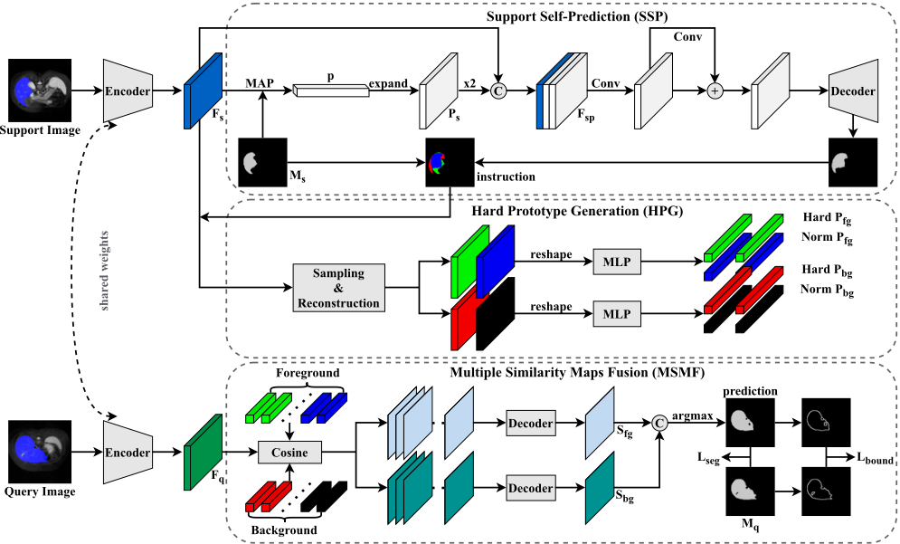
The proposed CoW is a dual-path architecture where similar operations are performed, one for segmenting foreground regions and the other for background. The framework comprises following primary components: (1) a generic feature encoder shared by the support and query images for extracting features; (2) an SSP module for acquiring a coarse predicted mask of the support image using global support prototype; (3) an HPG module for generating a specified number of hard prototypes for both foreground and background; (4) an MSMF module for fusing multiple similarity maps to get final segmenting mask of the query image. Figure 2 shows a more detailed pipeline of our method.
3.3 Support Self-Prediction
As shown in Figure 2, our proposed CoW starts by a parameter-sharing feature encoder denoted as fθ, which extracts features from both support and query images. We denote the support and the query features as Fs = fθ(Is) and Fq = fθ(Iq), Fs, Fq ∈ RC′×H′×W ′ , where C ′ is the channel depth of the feature, and H′ and W ′ denote the height and width of the feature respectively. Following the practice in Q-Net [Shen et al., 2023], we adopt ResNet-101 pre-trained on MS-COCO [Lin et al., 2014] as the backbone, and utilize the output feature of the third residual block.
In order to find out the weak feature points easily misclassified, which lead to over-segmentation and boundaryblurring, we devise a Support Self-Prediction (SSP) module to provide clues for them. Specifically, we firstly employ masked average pooling to generate a global support prototype ps ∈ R1×C′ from the support feature map Fs:
where Fs is resized to the size of corresponding mask Ms. ⊙ denotes the Hadamard product, and (h, w) is the pixel position. Then we duplicate and expand the support prototype ps to the same size as Fs, represented as Fp, which is subsequently concatenated with Fs to generate a new feature map:
where Concat(·) denotes the concatenation operator.
Next, the similarity map for the support image is generated after passing through the feature processing module and the decoder that adopts single-scale residual layers following an
where Ssupport ∈ R1×H′×W ′ is the predicted support similarity map. FPM(·) is the feature processing operation and D(·; ψ) means the support decoder parameterized with ψ. After that, we generate the predicted support mask ˆMs through a concatenation operation followed by an argmax operation:
where Ssupport is upsampled to (H,W) in advance and 1 - Ssupport represents the background similarity map.
For the purpose of finding weaker feature points in the support feature map, we adopt a cross-entropy loss on SSP module, which is written as:
where ˆM bg s = 1 - ˆM fg s , and the superscript fg and bg is the indicator for the foreground and background respectively.
Finally, we calculate the position of weak feature points and normal ones borrowing information from both predicted support mask ˆMs and support ground truthMs. This process can be mathematically expressed as:
where the superscript hf, hb, nf, nb refers to hard foreground, hard background, normal foreground and normal background respectively.
3.4 Hard Prototypes Generation
As opposed to previous works that employ multiple normal prototypes, which inevitably loses part of the detailed information and inadequately represents the overall feature distribution within a class, we devise a novel Hard Prototypes Generation (HPG) module to generate multiple hard prototypes for both foreground and background to guarantee full use of the support information. We will take the example of generating hard foreground prototypes as described below.
Building on the weak feature points instruction provided by the SSP module, we firstly remove all support feature points except for those belonging to hard foreground, which can be described as:
where ⊙ denotes element-wise multiplication.
Next, we reshape the features of hard foreground region, denoted as Dhf = [d1hf , d2hf , ..., dNhf hf ] ∈ RNhf×C′ . Then, a random sampling operation is performed on Dhf to extract some hard foreground points D′hf . This process can be expressed as:
where F(·) is a random sampling function and N is the number of D′hf .
Subsequently, we populate the hard foreground feature map F hf s withD′hf whereM hf s = 0 and retain original weak foreground feature points, which can be summarized mathematically in the following formulation:
where (h, w) denotes the spatial position of the pixel.
After that, we acquire a reconstructed hard foreground feature map where all feature points exclusively pertain to the hard foreground. In order to generate multiple hard foreground prototypes that fully capture the feature information, we pass the reconstructed F hf s through a lightweight MLP which is composed of a fully connected layer, a ReLU activation layer, and another fully connected layer. This process can be denoted as:
where MLP (·; ϕ) represents the MLP module parameterized with ϕ. The hard foreground feature map is reshaped to the dimension of HW × C ′ before being fed into the MLP and Phf ∈ RNhf×C′ denotes generated Nhf hard foreground prototypes.
Notably, the aforementioned procedure for generating hard prototypes also applies to hard background, normal foreground and background, namely Phb, Pnf , Pnb. Eventually, we concatenate the generated hard prototypes with normal ones and corresponding global support prototype for foreground and background respectively, which can be formu-
where ⊕ denotes the concatenation operation. pfg s and pbg s are support foreground and background prototypes generated via MAP. Pfg ∈ RNfg×C′ and Pbg ∈ RNbg×C′ are final representative prototypes used for predicting the foreground and background similarity maps of the query image respectively.
3.5 Multiple SimilarityMaps Fusion
In previous FSMIS tasks, researchers commonly leverage a single prototype or multiple normal prototypes to make predictions for the query image directly based on cosinesimilarity. However, there exist extreme imbalance between foreground and background in medical image and lost information in the masked feature, which easily lead to misclassified foreground and background points. To tackle this challenge, we design a Multiple Similarity Maps Fusion (MSMF) module, which fuses similarity maps generated by multiple prototypes obtained from HPG module, thus making more accurate segmentation.
First of all, we calculate the similarity maps between the multiple foreground and background prototypes, and the query image respectively:
where Sfg ∈ RNfg×H′×W ′ and Sbg ∈ RNbg×H′×W ′ denote the generated similarity maps for foreground and background of the query respectively.
Then, both Sfg and Sbg will be fed into a lightweight decoder to fuse multiple similarity maps, thereby generating the foreground prediction map and background prediction map. This process can be denoted as:
where D1(·; ψ1) and D2(·; ψ2) denote a straightforward decoder based on convolutional neural network with parameter ψ1 and ψ2. ˆM fg q ∈ R1×H′×W ′ and ˆM bg q ∈ R1×H′×W ′ are the final single predicted similarity map for query foreground and background respectively.
Finally, we upsample ˆM fg q and ˆM bg q to the size of (H,W) and integrate them by utilizing the concatenation operation and a softmax layer to get the final prediction, as follows:
where sof tmax(·) executes along the channel dimension and ˆMq ∈ R2×H×W will eventually be processed by an argmax operation to get the final segmentation mask of the query image.
3.6 Loss Function
In order to quantify the dissimilarity between the predicted and ground truth, we employ the binary cross-entropy loss as the segmentation loss for each training episode:
where Lseg works as the primary loss of our proposed CoW.
Following common practice [Wang et al., 2019; Ouyang et al., 2020], we inversely predict labels of the support images by using query images as the support set, then build a prototype alignment regularization loss, which is calculated as follows:
Additionally, we employ the intra-class loss to help diminish intra-class variation of the support and query and the interclass loss to improve discrimination among different classes, both enhancing the representativeness of our generated hard and normal prototypes for foreground and background, which is formulated as:
where the superscripts s and q denote the support and query image, cos is the cosine similarity, and max(·) means taking the maximum.
Furthermore, to get a more precise predicted mask, we devise a boundary loss to refine the segmentation boundary. Specifically, we generate the boundary map of ground truth and predicted mask through a maxpool operation, denoted as M b q and ˆM b q . Then, we calculate f1-score between them and get final boundary loss Lbound as follows:
where BF1(·, ·) computes the f1-score between input pair.
Overall, the loss function for each training episode is defined to be L = Lseg + Lalign + λ0Lbound + λ1(Lintra + Linter + Lssp), where λ0, λ1 are the balancing coefficients.
4 Experiment
4.1 Datasets, Settings and EvaluationMetrics
Datasets. To demonstrate the superiority of our method under different scenarios, we perform evaluations on three representative publicly available datasets: abdominal organs segmentation for MRI and CT (Abd-MRI [Kavur et al., 2021] and Abd-CT [Landman et al., 2015]) and cardiac segmentation for MRI (CMR [Zhuang, 2018]). The detailed introduction and split strategy is depicted in [Zhu et al., 2023].
Settings. Themajority of FSMISmodels follow the settings in the work [Ouyang et al., 2022] to evaluate their performance. In order to make a fair comparison, we also adopt the two experimental settings outlined in SSL-ALPNet [Ouyang et al., 2020] and ADNet [Hansen et al., 2022].
EvaluationMetrics. Following the common practice [Roy et al., 2020] in FSMIS, we employ the mean Sorensen-Dice coefficient (DSC) to compare the prediction to the ground truth. It measures the effectiveness of the same area between the predicted mask and the ground-truth.
4.2 Implementation Details
Following the practice in SSL-ALPNet [Ouyang et al., 2020], the experiments are conducted based on a 1-way 1-shot setting with 5-fold cross-validation. Initially, pseudo labels are generated for training by leveraging 3D superpixel clustering. After that, we reshape the size of the 2D slice from the 3D scanned image to 256 × 256 for Abd-MRI and CMR and 257 × 257 for Abd-CT. The total number of generated hard and normal prototypes for foreground and background are set to 100 and 600 respectively. We set the initial learning rate to 0.001, the decay rate to 0.9, and the total number of required iterations to 50K, containing 5000 iterations each epoch. The balancing coefficients λ0 and λ1 are set to 0.5 and 0.3 respectively in our experiment.
| Setting | Method | Reference | Abd-MRI | Abd-CT | ||||||||
|---|---|---|---|---|---|---|---|---|---|---|---|---|
| Liver | RK | LK | Spleen | Mean | Spleen | RK | LK | Liver | Mean | |||
| PA-Net | CVPR'19 | 50.40 | 32.19 | 30.99 | 40.58 | 38.53 | 36.04 | 21.19 | 20.67 | 49.55 | 31.86 | |
| SSL-ALPNet | ECCV'20 | 76.10 | 85.18 | 81.92 | 72.18 | 78.84 | 70.96 | 71.81 | 72.36 | 78.29 | 73.35 | |
| SR&CL | MICCAI'22 | 80.23 | 87.42 | 79.34 | 76.01 | 80.77 | 73.41 | 71.22 | 73.45 | 76.06 | 73.53 | |
| Q-Net | IntelliSys'23 | 81.74 | 87.98 | 78.36 | 75.99 | 81.02 | 77.81 | 70.98 | 73.83 | 76.37 | 74.75 | |
| 1 | CAT-Net | MICCAI'23 | 75.02 | 83.23 | 75.31 | 67.31 | 75.22 | 66.02 | 64.56 | 68.82 | 80.51 | 70.88 |
| RPT | MICCAI'23 | 82.86 | 89.82 | 80.72 | 76.37 | 82.44 | 79.13 | 72.58 | 77.05 | 82.57 | 77.83 | |
| GMRD | TMI'24 | 81.42 | 90.12 | 83.96 | 76.09 | 82.90 | 78.31 | 74.46 | 81.70 | 79.60 | 78.52 | |
| DSPNet | MIA'24 | 75.06 | 85.37 | 81.88 | 70.93 | 78.31 | 69.31 | 74.54 | 78.01 | 69.32 | 72.79 | |
| MSFSeg | MICCAI'24 | 76.11 | 88.10 | 84.18 | 77.12 | 81.38 | 73.64 | 78.41 | 81.11 | 78.91 | 78.02 | |
| Ours (CoW) | - | 81.55 | 90.27 | 85.58 | 79.00 | 84.10 | 83.56 | 80.46 | 83.60 | 82.35 | 82.49 | |
| PA-Net | CVPR'19 | 42.26 | 38.64 | 53.45 | 50.90 | 46.33 | 29.59 | 17.37 | 32.34 | 38.42 | 29.43 | |
| SSL-ALPNet | ECCV'20 | 73.05 | 78.39 | 73.63 | 67.02 | 73.02 | 60.25 | 54.82 | 63.34 | 73.65 | 63.02 | |
| SR&CL | MICCAI'22 | 75.55 | 84.24 | 77.07 | 73.73 | 77.65 | 67.36 | 63.37 | 67.39 | 73.63 | 67.94 | |
| Q-Net | IntelliSys'23 | 78.25 | 65.94 | 64.81 | 65.37 | 68.59 | 68.10 | 61.12 | 63.32 | 80.49 | 68.26 | |
| 2 | CAT-Net | MICCAI'23 | 78.98 | 78.90 | 74.01 | 68.83 | 75.18 | 67.65 | 60.05 | 63.36 | 75.31 | 66.59 |
| RPT | MICCAI'23 | 76.37 | 86.01 | 78.33 | 75.46 | 79.04 | 70.80 | 67.73 | 72.99 | 75.24 | 71.69 | |
| GMRD | TMI'24 | 80.25 | 86.66 | 78.65 | 73.25 | 79.70 | 75.30 | 76.17 | 77.40 | 80.39 | 77.32 | |
| DSPNet | MIA'24 | 78.56 | 82.01 | 76.47 | 68.27 | 76.33 | 66.48 | 63.55 | 68.46 | 69.16 | 66.17 | |
| MSFSeg | MICCAI'24 | 76.14 | 86.98 | 82.83 | 78.07 | 81.01 | 75.21 | 77.36 | 79.24 | 76.73 | 77.14 | |
| Ours (CoW) | - | 80.46 | 89.15 | 82.40 | 74.55 | 81.64 | 79.92 | 79.44 | 83.36 | 82.26 | 81.25 | |
| Method | Reference | CMR | |||
|---|---|---|---|---|---|
| LV-MYO | LV-BP | RV | Mean | ||
| PA-Net | CVPR'19 | 25.18 | 58.04 | 12.86 | 32.02 |
| SSL-ALPNet | ECCV'20 | 66.74 | 83.99 | 79.96 | 76.90 |
| SR&CL | MICCAI'22 | 65.83 | 84.74 | 78.41 | 76.32 |
| Q-Net | IntelliSys'23 | 65.92 | 90.25 | 78.19 | 78.15 |
| CAT-Net | MICCAI'23 | 66.85 | 90.54 | 79.71 | 79.03 |
| RPT | MICCAI'23 | 66.91 | 89.90 | 80.78 | 79.19 |
| GMRD | TMI'24 | 67.04 | 90.00 | 80.29 | 79.11 |
| DSPNet | MIA'24 | 64.91 | 87.75 | 79.73 | 77.46 |
| Ours (CoW) | - | 68.41 | 89.25 | 82.33 | 80.00 |
4.3 Comparison with SOTAMethods
For the purpose of convincingly demonstrating the superiority and effectiveness of our proposed CoW, we compare our method with several existing state-of-the-art methods, including PA-Net [Wang et al., 2019], SSL-ALPNet [Ouyang et al., 2020], SR&CL [Wang et al., 2022], CAT-Net [Lin et al., 2023], Q-Net [Shen et al., 2023], RPT [Zhu et al., 2023], GMRD [Cheng et al., 2024], DSPNet [Tang et al., 2024] and MSFSeg [Zheng et al., 2024], from the perspective of segmentation performance under two experimental settings. In this paper, considering that most researchers commonly adopt the PA-Net [Wang et al., 2019] as the baseline and the settings in SSL-ALPNet [Ouyang et al., 2020] to evaluate their performance, we also follow them to ensure a fair comparison.
| Baseline | SSP | HPG | MSMF | Abd-MRI | ||||
|---|---|---|---|---|---|---|---|---|
| Liver | RK | LK | Spleen | Mean | ||||
| � | � | � | � | 50.40 | 32.19 | 30.99 | 40.58 | 38.54 |
| � | � | � | � | 80.29 | 88.57 | 81.38 | 75.52 | 81.44 |
| � | � | � | � | 81.55 | 90.27 | 85.58 | 79.00 | 84.10 |
| Lintra | Linter | Lbound | Lssp | Abd-MRI | ||||
|---|---|---|---|---|---|---|---|---|
| Liver | RK | LK | Spleen | Mean | ||||
| � | � | � | � | 80.77 | 89.12 | 77.68 | 73.57 | 80.29 |
| � | � | � | � | 80.88 | 89.91 | 78.22 | 75.13 | 81.04 |
| � | � | � | � | 80.91 | 89.95 | 79.62 | 75.74 | 81.56 |
| � | � | � | � | 81.16 | 90.22 | 83.91 | 78.27 | 83.39 |
| � | � | � | � | 81.55 | 90.27 | 85.58 | 79.00 | 84.10 |
As shown in Table 1 and Table 2, our CoW significantly outperforms all listed methods in terms of the mean dice score on three different datasets.
4.4 Ablation Studies
Effect of each component. To evaluate separate contributions of each component within our model, we present their positive contributions in Table 3. Our SSP module and HPG module significantly improve its performance on top of the baseline model [Wang et al., 2019], achieving a mean dice score of 81.44%, which is attributed to the combination of normal and hard prototypes carrying rich subject and boundary information. In addition, the MSMF module with a dualpath architecture that aims at fusing multiple similarity maps further improves the performance by 2.66%.
| Nhf | Nnf | Abd-MRI | ||||
|---|---|---|---|---|---|---|
| Liver | RK | LK | Spleen | Mean | ||
| 0 | 100 | 81.49 | 89.22 | 84.09 | 77.44 | 83.06 |
| 25 | 75 | 81.55 | 90.03 | 84.39 | 78.66 | 83.66 |
| 50 | 50 | 81.55 | 90.27 | 85.58 | 79.00 | 84.10 |
| 75 | 25 | 81.22 | 89.85 | 82.99 | 77.83 | 82.97 |
| 100 | 0 | 82.04 | 90.15 | 83.75 | 72.43 | 82.09 |
| Method | Abd-CT | |||||
|---|---|---|---|---|---|---|
| Fold0 | Fold1 | Fold2 | Fold3 | Fold4 | Mean | |
| SSL-ALPNet | 75.37 | 65.65 | 68.68 | 77.68 | 79.37 | 73.35 |
| PMM | 74.70 | 63.81 | 69.33 | 78.26 | 76.15 | 72.45 |
| K-means | 77.06 | 67.02 | 75.42 | 79.76 | 80.79 | 76.01 |
| GMRD | 79.30 | 72.62 | 76.92 | 80.20 | 83.55 | 78.52 |
| Ours (CoW) | 83.46 | 77.72 | 81.14 | 84.32 | 85.80 | 82.49 |
Effect of each loss. As can be seen from the last column in Table 4, each loss indeed makes a separate contribution to the final performance. Lintra and Linter achieve a total gain of 1.27% by improving discriminability of generated multiple prototypes. Particularly, Lbound gives a 1.83% increase due to its constraint on the segmentation boundary. Moreover, Lssp brings an additional gain of 0.71% for the reason that we can acquire more robust normal and hard prototypes making support self-prediction more precise.
Number of normal and hard foreground prototypes. We test the effect of the number for Phf and Pnf on the final performance of CoW. As shown in Table 5, the optimal number setting is half for each. By contrast, employing Phf or Pnf alone leads to a performance degradation of 2.01% and 1.04% respectively because they solely leverage singular subject or boundary information, thus causing a less comprehensive representation for each category.
Generatingmultiple prototypes. We compare our method with several previous works [Ouyang et al., 2020; Yang et al., 2020; Hartigan and Wong, 1979; Cheng et al., 2024] in Table 6. It is apparent that our CoWachieves the best performance, surpassing the suboptimal GMRD by 3.97%, for the reason of focusing more attention to weak boundary details.
4.5 Visualization
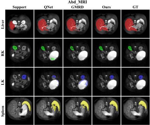
Qualitative Results. To better demonstrate the superiority of our method, qualitative results of our model and other models, including Q-Net [Shen et al., 2023] and GMRD [Cheng et al., 2024], on Abd-MRI are shown in Fig. 3 (More qualitative results on the CMR dataset and the AbdCT dataset can be found in Appendix).
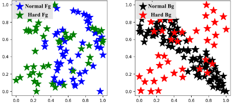
Distribution of Hard and Normal Prototypes. As depicted in Fig. 4, we visualize the generated hard and normal prototypes with t-SNE [Van der Maaten and Hinton, 2008]. It can be seen that normal foreground or background prototypes alone fail to well represent the entire distribution of their corresponding class. In contrast, the introduction of hard prototypes can compensate for such deficiency.
5 Conclusion
In this paper, we have proposed to mine hard prototypes by concentrating on weak features for few-shot medical image segmentation. It alleviates the challenge of current FSMIS methods that generate multiple prototypes solely through random sampling and local averaging, often failing to give a complete representation of corresponding category distribution. Additionally, our model includes a powerful edge constraint, which can further ensure a clearer segmentation boundary. Numerous experimental results also demonstrate that our method can capture more comprehensive class distribution and precisely segment the intricate organs in medical images. We believe that our model has the potential to assist in the diagnosis of rare disease and improve the efficiency of medical treatment.
Acknowledgments
This work was partly supported by the National Natural Science Foundation of China (NSFC) under Grant No. 62371235, and partly by the Key Research and Development Plan of Jiangsu Province (Industry Foresight and Key Core Technology Project) under Grant BE2023008-2.
@inproceedings{ijcai2025p139,
  title     = {Concentrate on Weakness: Mining Hard Prototypes for Few-Shot Medical Image Segmentation},
  author    = {Jiang, Jianchao and Zhang, Haofeng},
  booktitle = {Proceedings of the Thirty-Fourth International Joint Conference on
               Artificial Intelligence, {IJCAI-25}},
  publisher = {International Joint Conferences on Artificial Intelligence Organization},
  editor    = {James Kwok},
  pages     = {1242--1250},
  year      = {2025},
  month     = {8},
  note      = {Main Track},
  doi       = {10.24963/ijcai.2025/139},
  url       = {https://doi.org/10.24963/ijcai.2025/139},
}
TY - CPAPER TI - Concentrate on Weakness: Mining Hard Prototypes for Few-Shot Medical Image Segmentation AU - Jiang, Jianchao AU - Zhang, Haofeng T2 - Proceedings of the Thirty-Fourth International Joint Conference on Artificial Intelligence, IJCAI-25 PB - International Joint Conferences on Artificial Intelligence Organization PY - 2025 SP - 1242 EP - 1250 DO - 10.24963/ijcai.2025/139 UR - https://doi.org/10.24963/ijcai.2025/139 ER -Copied
Machine-readable versions of this paper, for tools and AI agents:





