
Large-Scale Trade-Off Curve Computation for Incentive Allocation with Cardinality and Matroid Constraints
Proceedings of the Thirty-Fourth International Joint Conference on Artificial Intelligence. Main Track. Pages 2575-2582.
https://doi.org/10.24963/ijcai.2025/287
Keywords
- Constraint Satisfaction and Optimization: CSO: Constraint satisfaction
- Constraint Satisfaction and Optimization: CSO: Constraint optimization problems
- Constraint Satisfaction and Optimization: CSO: Constraint programming
- Constraint Satisfaction and Optimization: CSO: Applications
Abstract
We consider a large-scale incentive allocation problem where the entire trade-off curve between budget and profit has to be maintained approximately at all time. The application originally comes from assigning coupons to users of the ride-sharing apps, where each user can have a limit on the number of coupons been assigned. We consider a more general form, where the coupons for each user forms a matroid, and the coupon assigned to each user must be an independent set. We show the entire trade-off curve can be maintained approximately in near real time.
- [Agarwal et al., 1998] P.K. Agarwal, D. Eppstein, L.J. Guibas, and M.R. Henzinger. Parametric and kinetic minimum spanning trees. In Proceedings 39th Annual Symposium on Foundations of Computer Science (Cat. No.98CB36280), pages 596-605. IEEE Comput. Soc, 1998.
- [Blelloch, 1991] Guy E. Blelloch. Prefix sums and their ap- plications, chapter 1. Morgan Kaufmann, Oxford, Eng- land, 1991.
- [Calinescu et al., 2011] Gruia Calinescu, Chandra Chekuri, Martin Pál, and Jan Vondrák. Maximizing a Monotone Submodular Function Subject to a Matroid Constraint. SIAM Journal on Computing, 40(6):1740-1766, January 2011.
- [Camerini and Vercellis, 1984] Paolo M. Camerini and Carlo Vercellis. The matroidal knapsack: A class of (often) well-solvable problems. Operations Research Letters, 3(3):157-162, 1984.
- [Carstensen, 1983] Patricia J. Carstensen. Complexity of some parametric integer and network programming prob- lems. Mathematical Programming, 26(1):64-75, May 1983.
- [Chan, 1999] Timothy M. Chan. Remarks on k-level algo- rithms in the plane. Manuscript, 1999.
- [Cole, 1987] Richard Cole. Slowing down sorting networks to obtain faster sorting algorithms. Journal of the ACM, 34(1):200-208, January 1987.
- [Dey, 1998] T. K. Dey. Improved bounds for planar k -sets and related problems. Discrete & Computational Geome- try, 19(3):373-382, Mar 1998.
- [Doron-Arad et al., 2024] Ilan Doron-Arad, Ariel Kulik, and Hadas Shachnai. Lower Bounds for Matroid Optimization Problems with a Linear Constraint. In Karl Bringmann, Martin Grohe, Gabriele Puppis, and Ola Svensson, editors, 51st International Colloquium on Automata, Languages, and Programming (ICALP 2024), volume 297 of Leibniz International Proceedings in Informatics (LIPIcs), pages 56:1-56:20, Dagstuhl, Germany, 2024. Schloss Dagstuhl -Leibniz-Zentrum für Informatik.
- [Dyer, 1984] M. E. Dyer. An O(n) algorithm for the multiple-choice knapsack linear program. Mathematical Programming, 29(1):57-63, May 1984.
- [Efron, 1965] Bradley Efron. The convex hull of a random set of points. Biometrika, 52(3/4):331-343, 1965.
- [Eisner and Severance, 1976] Mark J. Eisner and Dennis G. Severance. Mathematical Techniques for Efficient Record Segmentation in Large Shared Databases. Journal of the ACM, 23(4):619-635, October 1976.
- [Eppstein, 1998] D. Eppstein. Geometric Lower Bounds for Parametric Matroid Optimization. Discrete & Computa- tional Geometry, 20(4):463-476, December 1998.
- [Erdös et al., 1973] P. Erdös, L. Lovász, A. Simmons, and E.G. Straus. Chapter 13 -dissection graphs of planar point sets. In Jagdish N. Srivastava, editor, A Survey of Combi- natorial Theory, pages 139-149. North-Holland, 1973.
- [Fife and Oxley, 2017] Tara Fife and James Oxley. Laminar matroids. European Journal of Combinatorics, 62:206- 216, 2017.
- [Javaudin et al., 2022] Lucas Javaudin, Andrea Araldo, and Andrù de Palma. Large-scale allocation of personalized incentives. In 2022 IEEE 25th International Confer- ence on Intelligent Transportation Systems (ITSC), page 4151-4156. IEEE Press, 2022.
- [Lovász, 1971] L. Lovász. On the number of halving lines. Annales Universitatis Scientiarum Budapestinen- sis de Rolando Eőtvős Nominatae Sectio Mathematica, 14:107-108, 1971.
- [Megiddo, 1983] Nimrod Megiddo. Applying parallel com- putation algorithms in the design of serial algorithms. J. ACM, 30(4):852-865, oct 1983.
- [Murty, 1980] Katta G. Murty. Computational complexity of parametric linear programming. Mathematical Program- ming, 19(1):213-219, December 1980.
- [Pisinger, 2001] David Pisinger. Budgeting with bounded multiple-choice constraints. European Journal of Oper- ational Research, 129(3):471-480, 2001.
- [Schrijver, 2002] Alexander Schrijver. Combinatorial Opti- mization: Polyhedra and Efficiency. Springer, Berlin, Ger- many, 2003 edition, 2002.
- [Sinha and Zoltners, 1979] Prabhakant Sinha and Andris A. Zoltners. The multiple-choice knapsack problem. Opera- tions Research, 27(3):503-515, 1979.
- [Sviridenko et al., 2014] Maxim Sviridenko, Jan Vondrák, and Justin Ward. Optimal approximation for submodular and supermodular optimization with bounded curvature, December 2014. arXiv:1311.4728 [cs].
- [Tokuyama, 2001] Takeshi Tokuyama. Minimax parametric optimization problems and multi-dimensional parametric searching. In Proceedings of the Thirty-Third Annual ACM Symposium on Theory of Computing, STOC '01, page 75-83, New York, NY, USA, 2001. Association for Com- puting Machinery.
- [Tóth, 2001] G. Tóth. Point Sets with Many k-Sets. Dis- crete & Computational Geometry, 26(2):187-194, January 2001.
- [Wang and Shmoys, 2019] Shujing Wang and David Shmoys. How to solve a linear optimization problem on incentive allocation?, Sep 2019.
- [Zadeh, 1973] Norman Zadeh. A bad network problem for the simplex method and other minimum cost flow algo- rithms. Mathematical Programming, 5(1):255-266, De- cember 1973.
- [Zemel, 1984] Eitan Zemel. An o(n) algorithm for the linear multiple choice knapsack problem and related problems. Information Processing Letters, 18(3):123-128, 1984.
References were extracted automatically from the PDF and may contain errors.
Full text extracted automatically from the PDF; figures, tables and equations may differ. The PDF is the version of record.
1 Introduction
In the current age, we are dealing with increasingly large incentive allocation problems. One is given a fixed amount of budget to allocate to different incentives to maximize some objective. A prototypical example is assigning a single coupon to each rider in ridesharing apps, where each assignment uses up some marketing budget, and increase some metric such as rides or driving hours [Wang and Shmoys, 2019]. For example, an incentive allocation problem under cardinality constraints can be formalized as the following integer program.
For each agent i, there is a candidate incentive set consisting of coupons, where the value and cost of the jth coupon is vij and cij, respectively. The goal is to select at most k coupons for each agent and to make sure that the total cost of the selected coupons does not exceed the budget B while maximizing the total value of those coupons.
The problem is a variant of the knapsack problem, and computing the exact optimum is NP-hard. However, the fractional optimum is very close to the integer optimum, even if there are strong constraints in the allocation [Camerini and Vercellis, 1984]. Hence, in this article, we only consider finding the fractional optimum.
The allocation under a fixed budget is often insufficient for decision and analytic purposes. For example, the company might want to decide on the total budget for a campaign. A data scientist might need to know how much marketing spend is required to obtain an expected profit. These questions can all be answered if the entire trade-off curve of the budget vs profit can be computed. There can be more complicated cases where the decider might not be a person but an algorithm. Consider the following case: The ridesharing company wants to allocate a budget to two campaigns, one of which is incentive allocation. We are optimizing maxx f(x) + g(B - x), where f would map to the trade-off curve in the incentive allocation problem and g is the value of the other campaign. g can be complicated and in that case an algorithm optimizing the sum would evaluate g at many different values of x. Implementing such an algorithm will be a lot faster and easier if we can compute the trade-off curve f quickly. Moreover, the curve is not static: In practice, the cost and value of a coupon are usually predicted by algorithms or models. An agent might take a certain action, say take a ride, and the model would change its predictions of the expected profit of each incentive associated with the agent.
Hence, we investigate the dynamic incentive allocation trade-off curve problem, where the entire trade-off curve has to be maintained, while supporting updates(insertions and deletions) of agents' incentives. In practice, the number of agents is large (in the millions), the choices of incentives for each agent is relatively small (a few hundred), and no agent is critical to the objective. That is, removing any agent would not significantly impact the objective. Also, we assume each agent is independent: the incentives to one do not affect others.
Generally, for each agent, there can be constraints on the allocation of incentives. We consider some examples in the ridesharing apps. A user can be assigned at most one of the incentives (multiple choice constraint). A user can be assigned no more than p incentives (cardinality constraint). A user can have 2 incentives for weekends, and 2 incentives for weekdays, but only 3 incentives in total (special case of matroid constraint). The most general constraints are given as an arbitrary family of feasible subset of incentives. Our work would also consider how the problem changes under different constraints, but we mainly focus on cardinality and matroid constraints.
Finally, we want the implementation to be easily transferable to queries in a modern OLAP databases.
Previous Works. The (integral) incentive allocation problem for a fixed budget B is a knapsack problem with side constraints. Our work is concerned with the linear programming relaxation, the fractional version, of the knapsack problem.
When each agent is allocated exactly 1 incentive, it is also called the continuous multiple choice knapsack problem (CMCKP), and was widely studied. Sinha and Zoltners [Sinha and Zoltners, 1979] showed the optimum gap from the integral case is the value of a single incentive. Later, optimum linear time algorithm was discovered [Dyer, 1984; Zemel, 1984]. When each agent is required to be allocated exactly (or at most) p incentives, namely having cardinality constraint on the incentives, it is equivalent to the continuous bounded multiple choice knapsack problem (CBMCKP). CMCKP is the special case of CBMCKP when p = 1. Pisinger showed a reduction from CBMCKP to CMCKP, but running time depends on B [2001]. In the same paper, Pisinger used the Dantzig-Wolfe decomposition to devise a faster polynomial time algorithm. However, the algorithm's running time depends on the size of the value and the cost, therefore it is not a strongly polynomial time algorithm.
When the incentive for each agent must form an independent set (or a base) in a matroid, it is the (continuous) matroidal knapsack problem [Camerini and Vercellis, 1984]. The running time for finding an optimum is O(m2 +T log m) time, where m is the number of incentives and T is the complexity of finding the optimum base for a given weighting of the elements in the matroid. After the technique of parametric search was introduced and improved [Megiddo, 1983; Cole, 1987], the running time was improved to O(T logm) [Tokuyama, 2001]. CBMCKP is a special case of the matroidal knapsack problem when the matroid is a p-uniform matroid. Although not explicitly stated, the matroid algorithm can be used for CBMCKP, and obtain an O(mlogm) time algorithm because it takes O(m) time to find the optimum base for a uniform matroid [Tokuyama, 2001]. See Table 1 for a comparison of results.
From another point of view, the incentive allocation problem can be considered a matroid optimization problem with an additional linear constraint. For general matroid this problem admits no fully polynomial-time approximation scheme [Doron-Arad et al., 2024].
For readers familiar with parametric or multi-objective optimization, it may also be helpful to view the trade-off curve as the Pareto curve between objectives. Under the multiobjective optimization framework, we are solving matroidal knapsack problem with an additional objective that minimize the total budget. Computing the trade-off curve can also be considered a sensitivity analysis problem, where the budget is the parameter whose sensitivity we are interested in. While these interpretations provide additional insight, our analysis is mainly conducted within the linear programs for the incentive allocation problem, as LPs better capture the properties of the problem and are easier to understand.
We are not aware of explicit computation of the entire trade-off curve except in the CMCKP case. A recent study in the transportation economics area [Javaudin et al., 2022] considered each agent must pick one of a few incentives, each having a different impact to social welfare. The regulator consults the entire trade-off curve for informed policymaking. The algorithm has a running time of O(mlogm). The result is static, as it does not concern about updating the curve when individual incentive changes.
Our contribution. We show that the entire incentive allocation trade-off curve is piecewise linear and concave. We construct a conceptually simple method to maintain the curve under different constraints, while allowing updates in logarithmic time with respect to number of fundamental changes of the trade-off curve. In particular,
- In the multiple choice constraint case, the result matches the current fastest algorithm for static trade-off curve, but our implementation allows dynamic updates.
- In the cardinality constraint case, we show the entire trade-off curve can be computed with O(logm) amortized time per breakpoint.
- We also observe that our problem is related to the klevel problem in computational geometry and parametric matroid optimization. The connection shows a subquadratic bound to the number of breakpoints in the trade-off curve, when previously the bound is quadratic.
Finally, we show part of the algorithm can be handled by modern OLAP database to avoid implementation complexity. As a preview, we will prove the following theorems.
Theorem 1. Consider an incentive allocation problem with a total of m incentives. If there is a cardinality p constraint on each agent, and k is the number of breakpoints on the tradeoff curve, then k = O(mp1/3 ), and the trade-off curve can be computed in O((k +m) logm) time.
Theorem 2. Consider an incentive allocation problem with a total of m incentives. If there is a matroid constraint on each agent, each matroid has rank at most p, and k is the number of breakpoints on the trade-off curve, then k = O(mp1/3 ), and the trade-off curve can be computed in O(T k+k log m) time, where T is the time to compute the optimum weight base.
Theorem 3. If the slope-difference form of trade-off curve after an update differs from previous trade-off curve at t positions, then the update takes O(t log k) time, where k is the total number of breakpoints in the curve.
Assuming each agent is only available for a few hundred incentives, then each update of an agent, t would be around the same number, which would make the running time nearreal time.
| Constraint Type | Result | Fixed budget | Trade-off curve | Dynamic |
|---|---|---|---|---|
| Multiple Choice | [Dyer, 1984; Zemel, 1984] [Javaudin et al., 2022] Theorem 1 | O(m) - | - O(m log m) O(m log m) | - No Yes |
| - | ||||
| Cardinality | [Pisinger, 2001] | O(m log V C) | - | - |
| [Pisinger, 2001] | O(mp + nB) | - | - | |
| [Tokuyama, 2001] | O(m log m) | - | - | |
| Theorem 1 | - | O((k +m) logm) | Yes | |
| Matroid | [Camerini and Vercellis, 1984] | O(m2 +T logm) | - | - |
| [Tokuyama, 2001] | O(T logm) | - | - | |
| Theorem 2 | - | O(Tk +k logm) | Yes |
2 Preliminaries
We define [n] = {1, . . . , n}. Let x ∈ Rm, if I ⊆ [m], then xI is the vector of length |I| obtained by deleting elements outside the index set. x(I) = ∑i∈I xi. Conv(X) is the convex hull of X.
2.1 Prefix Sum and Piecewise Linear Convex Function Representations
Given a sequence of elements a1, . . . , an and some associative operation ⊕, the prefix sum is the sequence b1, . . . , bn, such that b1 = a1, and bi = bi-1 ⊕ ai. The prefix sum data structure maintains the corresponding prefix sums under updates of the original sequence, allowing query of each prefix sum value and binary search (if monotonic) in O(log n) time [Blelloch, 1991].
Let f : [0,∞) → R be a piecewise linear convex function with n breakpoints (0 is always a breakpoint). There are 3 different forms that capture almost all information of f, and one can transform between them using prefix sum or even easier operations.
- The slope-difference form SD(f) = {(x1,∆1), . . . , (xn,∆n)}, where x1 = 0, ∆1 is the left most slope of f, and xi is the ith breakpoint, and ∆i for i > 1 is the difference between the right slope and the left slope.
- The slope form S(f) = {(x1, s1), . . . , (xn, sn)}. Again, xi are the breakpoints, and si = ∑ij=1 ∆i is the right slope at point xi.
- The value form V (f) = {(x1, f(x1) - f(0)), . . . , (xn, f (xn) - f (0))}.
Note that the previous forms also require the value of f(0) in order to uniquely recover the function, hence it has to be stored elsewhere. One can write the prefix sum data structure by hand, such that the original sequence is the slopedifference form, and any update in slope-difference form would propagate to slope and value form.
The slope-difference form is also easy for sums. SD(f+g) is simply SD(f)∪SD(g) if f and g do not share breakpoints, otherwise, sum the slope-difference at the breakpoint. For simplicity of exposition, we assume the functions we sum do not share breakpoints. This also allows one to maintain f = ∑i fi easily by taking the union.
By maintaining a function, we means that the following question can be answered quickly
- Evaluate: Given x, return f(x).
- Inverse: Given y, find smallest x such that f(x) = y.
- Output: Given x and y, output the function f restricted on [x, y].
If f is the trade-off curve, then "Evaluate" can answer how much value can be obtained for a given budget, and "Inverse" can answer how much budget is required for a particular value.
2.2 Matroids
A matroid M = (E, I) is a set system over ground set E, and I consists of subsets of E, such that the following properties hold.
- ∅ ∈ I.
- A ∈ I, then every subset of A is in I.
- If A,B ∈ I, and |A| > |B|, then there is x ∈ A \ B, such that B ∪ {x} ∈ I.
The sets in I are called independent sets, and the maximal independent sets are called bases. The rank function r associated with M is defined as r(S) = max{|S ′ | | S′ ⊆ S, S′ ∈ I}, the size of the largest independent set contained in S. The rank of the matroid is defined as r(E).
A matroid is a p-uniform matroid if there exists an integer p, such that every set of size at most p is an independent set.
2.3 Problem and Properties
Consider an (integral) incentive allocation problem with n agents. The ith agent has a candidate set of incentives, Ei. Each incentive e has a cost ce and a value ve, respectively. To model constraints, let Fi be the feasible subsets of Ei, which can be encoded as a set of binary vectors. Let mi = |Ei| and m = ∑i mi. The problem is to choose a feasible set of incentives for each agent, such that the sum of value of all the chosen incentives is maximized while the total cost does not exceed budget B.
The (integral) incentive allocation problem can be formulated as the following integer program (IP):
Define ¯ τ(B) to be the objective value of the above integer program. The exact trade-off curve is the function ¯ τ as B ranges from 0 to ∞. Finding ¯ τ(B) is NP-hard, therefore we consider the linear programming relaxation instead. This is shown below.
Define τ(B) to be the objective value of the linear programming relaxation of the integer program IP. We call τ the (fractional) trade-off curve.
One can reduce the problem to multiple choice knapsack similar to the reduction by Pisinger [2001], and show τ(B)- ¯ τ(B) ≤ maxi{∑e∈Ei ve}. That is, the maximum difference is at most the value a single agent can provide. If additionally, we know Fi forms a matroid for each i, then a stronger result exists: the difference is at most the value of a single incentive [Camerini and Vercellis, 1984]. Namely, τ(B) - ¯ τ(B) ≤ ∥v∥∞.
Because in large-scale problems such as coupon assignment, single agent's value is small compared to the objective. Therefore, τ is a very close approximation of ¯ τ. Hence, our work is to maintain the function τ .
3 Algorithm
The algorithm is conceptually simple. The computation gets broken into two independent parts, allowing for greater parallelization and customization.
The idea is to compute a signature function for each agent. The signature functions can be computed in parallel, completely independently. The sum of the signature functions is the function we will maintain, and we show how to use the sum to obtain the desired information on τ .
3.1 From Signature Functions to Trade-Off Curve
We start with the most general form of the problem Equation (1). Let Pi = Conv(Fi). Consider we have n polyhedrons P1, . . . , Pn together with disjoint index sets E1, . . . , En with their union [m].
Consider the following linear program,
We define fi(λ) = max{(vEi - λcEi )x|x ∈ Pi}, and we call it the signature function of agent i. The signature function fi is piecewise linear and convex since it is the upper envelope of line arrangement {lx(λ) = vEi · x-λcEi · x|∀x ∈ Pi}.
Let f = ∑i fi. The Lagrangian dual of the linear program is therefore
Note that each fi is a piecewise linear convex function, hence λB + f(λ) is also piecewise linear and convex.
Given the signature function fi for each agent, we have to maintain the function f = ∑i fi. Maintaining f itself is an easy task since it is just the sum of piecewise linear functions, the number of breakpoints is the total number of breakpoints for fi. If each fi is stored in slope-difference form, then f can be computed through a simple merge of the lists.
Theorem 4. τ is a piecewise linear concave function and τ (B) = minλ λB + f (λ).
This shows once we have the signature functions, the tradeoff curve is easy to compute through common techniques for manipulating piecewise linear functions. See the technical appendix for the full proof.
We have already established that τ is closely related to f. Next, we show how to maintain τ dynamically.
Assume f has k breakpoints and all three forms(value, slope and slope-difference) of f are given. We answer the following questions.
- Evaluate: For a fixed B, how to find τ(B)?
- Inverse: Find a B such that τ(B) = y.
- Update: Maintain τ after a single agent's incentive changes.
- Output: Output a contiguous piece of τ.
Evaluate. Bλ+f(λ) is a piecewise linear convex function, the minimum is at the first position where the slope becomes positive. Or in other words, find the first λ in f, where the slope is greater than -B. This can be processed easily by looking at the slope form of f and do a binary search, and it would take O(log k) time.
Inverse. The idea is to find τ(B1) ≤ y < τ(B2), such that B1 and B2 correspond to the two consecutive slopes of f. We can do binary search over the breakpoint of f to find the corresponding λ1 for B1. Finally, solve the linear equation Bλ1 - f(λ1) = y to obtain B.
Update. Assume information for agent i updates, then the only change is the signature function for that agent. Assume the new signature function after the update is gi. The new f is obtained by subtracting fi and adding gi successively. We could also save time by only updating the difference in fi and gi. Hence, the amount of time spent on update is bounded by the number of breakpoint changes times a log factor, and the time finding the new signature function.
Note that the function is stored in slope-difference form; hence, any update in which only t positions in the slopedifference form change takes O(t log k) time, which proves Theorem 3.
Output τ. Evaluating and finding the inverse are sufficient for most purposes, but if we do want to output a contiguous piece of τ that consists of at most t breakpoints, we can do so in O(log k + t) time. We know precisely for which B the curve τ changes in slope: a one to one correspondence with the breakpoints of f. Hence, we can first find the desired place in τ and output the breakpoints one by one by walking through the slope table of f.
Theorem 5. Given the signature functions for each agent, it takes O(k log k) time to compute a representation for τ, where k is the number of breakpoints in the trade-off curve.
The running time in Theorem 5 is obtained by merging signature functions of agents and depends on the output size. The complexity of maintaining the trade-off curve depends on how many breakpoints there are in f, which in turn is linearly related to the number of breakpoints in each signature function. The next step is to bound the number of breakpoints in the signature functions, and the time to compute it.
Because f decomposes as the sum of signature functions, we only have to focus on a single agent. So from this point on, we only consider the signature function for a single agent.
3.2 General Signature Function
In the most general case, we would define the signature function f(λ) to be the optimum of maxx{(v - λc) · x|x ∈ P}, where x is an m dimensional vector. This is the general parametric linear program. The number of breakpoints in f can be exponentially large, namely Ω(2√m) [Zadeh, 1973; Murty, 1980; Carstensen, 1983].
However, if the constraints in the question are matroids, the number of breakpoints is reasonably small, and can be computed quickly. To start, we focus on the cardinality constrained case.
3.3 Cardinality Constraint
Consider an agent who has m incentives E, and at most p of them can be allocated to the agent. The signature function is f(λ) = max{(v - λc) · x|1 · x ≤ p, 0 ≤ x ≤ 1}. For ease of manipulation later, we actually want equality. That is, the agent gets exactly p incentives. Indeed, we can add p dummy incentives with 0 value and 0 cost. Pisinger observed the number of possible slopes is upper bounded by m2 , hence showing f have at most O(m2 ) breakpoints [2001].
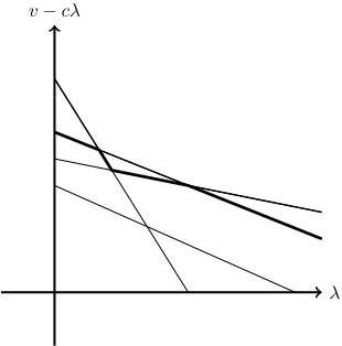
We use techniques from computational geometry to view this problem. Consider an arrangement of lines {ℓe | e ∈ E}, where ℓe(λ) = ve - λce for e ∈ E. f(λ) is the sum of p top most lines when x coordinate is λ. Therefore, in order to find f, it is sufficient to find the top p lines in the arrangement for each λ.
The simple brute force method is to first find all intersections of the lines, and sort them by x coordinate. In between each two consecutive intersections, the top p lines cannot change. So we calculate the top p lines on all x intervals formed by two consecutive intersections. Because there are O(m2 ) intersections, the number of breakpoints is also O(m2 ), which gives an alternative way to show Pisinger's bound. The bound is very loose, and next we show how the geometric view can improve the bound. The set of points that is the top pth point in an arrangement of lines is called the p-level [Erd¨os et al., 1973; Lov´asz, 1971]. 1-level is the upper envelope of the lines, which is the boundary of a convex space. However, for p > 1, it is not necessarily convex, see Figure 1. p-level is known to be computable in O(mlogm + k) time through clever computational geometry data structures [Chan, 1999], where k is the number of breakpoints of in the p-level. Observe that the slope of the signature function f can only change at the breakpoint of the p-level. Indeed, even when there are many line intersections above the p-level, the top p lines does not change, hence the sum would not change. The current best upper bound on the number of breakpoints of p-level is O(mp1/3 ) [Dey, 1998]. Together, it reflects f has O(mp1/3 ) breakpoints and can be computed in the same time as computing the p-level.
Theorem 6. A signature function of k breakpoints for p cardinality constrained incentive allocation trade-off curve can be computed in O(mlogm + k) time, and it has at most O(mp1/3 ) breakpoints.
The true upper bound for number of breakpoints in p-level might be much smaller. The currently known lower bound is only m2Ω(√log p) [T´oth, 2001]. Any improvement in the upper bound implies a better bound on the complexity of the trade-off curve.
3.4 Matroid Constraint
The agent must be assigned an independent set of incentives in a matroid over ground set E. Let |E| = m, r is the rank function, and p = r(E) is the rank of the matroid.
Using standard knowledge from matroid theory [Schrijver, 2002], f(λ) would be defined as the optimum of the following linear program, after adding dummy items with 0 cost and 0 value into every independent set.
For a fixed λ, this LP is finding the optimum weight base in a matroid, where the weight is w(e) = ve -λce. Breakpoints on f (λ) indicate that the matroid's optimum base changes due to the linear change in weights. The number of breakpoints on f is bounded by O(mp1/3 ) [Dey, 1998]. Unfortunately, unlike the cardinality case, there are matroids forcing Ω(mp1/3 ) breakpoints on the signature function [Eppstein, 1998].
To compute f, we need to find all breakpoints on f. However, for matroid constraints there is no existing efficient algorithm finding breakpoints on the signature functions for general matroids as the k-level algorithm for cardinality constraints.
Similar problem under graphic matroid has been studied in [Agarwal et al., 1998]. The authors use parametric search and sparsification techniques to find breakpoints efficiently. The techniques are limited to graphs and cannot be applied to general matroids. We achieve a running time of O(Tmp1/3 ) for general matroids by using the Eisner-Severance method, where T is the time complexity of finding optimum weight base in a matroid.
Eisner-Severance method is a simple algorithm for finding breakpoints on convex piecewise linear functions [Eisner and Severance, 1976]. Given any piecewise linear convex function f : R → R with k breakpoints and an oracle which computes f(λ) and arbitrary tangent line of f at λ. ES method finds all breakpoints on f with O(k) oracle calls. The method is as follows. We maintain a sequence of line segments L = {l1, ..., lk} of f. Initially, the sequence L = {l1, lk} contains the leftmost and rightmost segments. Denote by Λ the list of intersections of adjacent lines in L. ES method works by repeatedly adding line segments to L. In each iteration we check one intersection λi ∈ Λ and evaluate f(λi). Suppose λi is the intersection of line segments lt and lt+1. Note that λi is a breakpoint on f if and only if f(λi) = lt(λi) = lt+1(λi). Thus for every λ ∈ Λ, we can easily check if it is a breakpoint on f by calling the oracle at λ and performing several comparisons. If λ is a breakpoint on f , we remove λ from list Λ; Otherwise, there exists a new line segment lp that attains the maximum at λ among all lines in L and can be found using the oracle. We insert lp to L and add its intersections with adjacent lines to Λ. The algorithm terminates when Λ = ∅. The correctness of the algorithm is ensured by the correctness of the ES method.
Each intersection added to Λ gives us a breakpoint or a new line segment. Thus the total number of evaluations of f is O(k), where k = O(mp1/3 ) is the number of breakpoints.
For finding lp and evaluate f(λ), we need to find the optimal weight base which takes O(T). Thus the total time complexity of computing signature function for one agent with m incentives is O(Tmp1/3 ).
Our algorithm also leads to a simple proof that the optimal solution has at most two fractional variables. This fact can also be deduced from the proof of the integrality gap [Camerini and Vercellis, 1984].
Theorem 7. There exists an optimal solution to Equation (1) under matroid constraints with at most 2 fractional variables.
See the technical appendix for the proof.
3.5 Wrapping Up
Combining Theorem 6 and Theorem 5, we obtain the desired theorems.
Theorem 1. Consider an incentive allocation problem with a total of m incentives. If there is a cardinality p constraint on each agent, and k is the number of breakpoints on the tradeoff curve, then k = O(mp1/3 ), and the trade-off curve can be computed in O((k +m) logm) time.
Proof. Assume the ith agent has mi choices of incentives, and the breakpoint of the signature function is ki. By Theorem 6, the running time for computing all signature functions is O(∑i mi log mi +ki) = O(m log m+k). By Theorem 5, constructing the data structure for τ takes O(k log k) = O(k logm) time. So together we have the running time O(m log m + k + k log m) = O((m + k) log m).
By the above theorem, when p = 1, namely the multiple choice constrained case, k = O(m), and we obtain the desired O(mlogm) running time.
For matroid constraints, we get a more modest result.
Theorem 2. Consider an incentive allocation problem with a total of m incentives. If there is a matroid constraint on each agent, each matroid has rank at most p, and k is the number of breakpoints on the trade-off curve, then k = O(mp1/3 ), and the trade-off curve can be computed in O(T k+k log m) time, where T is the time to compute the optimum weight base.
Proof. Assume the signature function has ki breakpoints for agent i and m is the total number of incentives. The running time of computing one signature function is O(Tki). Computing all signature functions takes O(Tk) since ∑i Tki ≤ Tk. By Theorem 5, constructing the data structure for τ takes O(k log k) = O(k logm) time. So together we have the running time O(T k + k log m).
For practical purpose, once we have the signature functions for single agents, the trade-off curve can be easily computed with OLAP databases. See the Technical Appendix for details.
Next we discuss the work per update of a single agent. Each single agent update can only change breakpoints of the associated signature function. If s incentives are related to the agent, at most O(s4/3 ) breakpoint changes can happen, The update time would be O(s4/3 log k). As we assumed in the scenario, s is small because no agent is related to too many incentives, hence this would be a fast operation in modern systems.
4 Submodular Objective
In this section we discuss a more general case where the objective function is submodular instead of linear. Submodular objective function reflects the diminishing marginal gain phenomenon thus is closer to reality. In practice, agents usually receive incentives for free. We further assume that the submodular objective function g : 2E → R is monotone, nonnegative and satisfies g(∅) = 0. Thus, we are particularly interested in polymatroid objective functions.
The submodular incentive allocation problem can be formulated as follows:
where g : {0, 1}m → R is a polymatroid set function. We define the signature function for agent i to be fi(λ) = max {g(x) -λc · x|x ∈ Fi ∩ {0, 1}|Ei|}. The Lagrangian dual can be written as minλ≥0 Bλ + ∑i fi(λ).
Note that the properties of signature functions in Section 3.1 are independent of the objective function and constraints. Therefore, fi(λ) is piecewise linear and convex, even for submodular objectives. However, our algorithm does not extend to the submodular case.
Our method requires an efficient algorithm for evaluating fi(λ). For the submodular case, we need to solve a constrained submodular maximization problem to compute fi(λ). It is known that this problem is NP-hard [Calinescu et al., 2011], so we consider solving it approximately. g(x)-λc· x is still submodular for x but is not monotone. The best approximation rate is g(x)-λ·x ≥ (1-1/e)g(xOPT )-λ·xOPT in [Sviridenko et al., 2014]. However, the running time is impractical for implementations and currently no nontrivial upper bound is known for the number of breakpoints on fi.
5 Computational Results
Our paper is mostly theoretical, but we did an implementation to see how does theory fair in practice for the cardinality constraint case. Do we need to use advanced computational geometry tools to obtain good result in practice?
For cardinality case we implemented two algorithms, one is to use the optimum p-level data structure which runs in O((k +m) logm) time. The other is a simple scan line algorithm. The algorithm maintains the p-level by looking at all intersections with the current pth line, which gives an O(km) running time.
All tests were run on MacOS operating system with an M2Max cpu. Table 2 shows the average running time of 10 random instances each case, the numbers are drawn from a uniform sample.
The scan line algorithm is surprisingly good for small p. It is because in those cases k is actually very small, much smaller than m. There is an intuitive argument. If p = 1, then k is the same as the number of points on the convex hull of a uniform random sample of m points. The expected value is O(logm) [Efron, 1965]. Note as p becomes larger, for a random set of points k also becomes larger, and therefore the O(mk) algorithm suffers. Still, k is much smaller than m, and we get the optimum algorithm with a running time of O(m log m).
For the matroid case we tested our algorithm on laminar matroids. The laminar matroid is defined on a laminar family. Given a set E, a family A of subsets of E is laminar if for every two sets A, B ∈ A with A ∩ B ̸= ∅, either A ⊆ B or B ⊆ A. Define the capacity function c : A → R. The
| m | p = 20 | p = 40 | ||
|---|---|---|---|---|
| scan | opt | scan | opt | |
| 1×10³ | 0.000 | 0.000 | 0.000 | 0.001 |
| 5×10³ | 0.003 | 0.005 | 0.006 | 0.005 |
| 1×10⁴ | 0.008 | 0.010 | 0.014 | 0.012 |
| 5×10⁴ | 0.043 | 0.089 | 0.080 | 0.087 |
| 1×10⁵ | 0.094 | 0.216 | 0.173 | 0.223 |
| 5×10⁵ | 0.528 | 2.911 | 0.937 | 2.952 |
| 1×10⁶ | 1.147 | 7.291 | 1.989 | 7.140 |
| 1×10⁷ | 12.994 | 100.512 | 23.863 | 101.675 |
| m | p = 2000 | p = m/5 | ||
| scan | opt | scan | opt | |
| 1 × 10³ | - | - | 0.003 | 0.002 |
| 5×10³ | 0.137 | 0.027 | 0.091 | 0.02 |
| 1×10⁴ | 0.384 | 0.048 | 0.384 | 0.048 |
| 5×10⁴ | 2.634 | 0.187 | 9.531 | 0.326 |
| 1×10⁵ | 5.795 | 0.397 | 38.275 | 1.222 |
| 5×10⁵ | 33.760 | 3.398 | TLE | 10.500 |
| 1×10⁶ | 72.485 | 7.604 | TLE | 23.203 |
| TLE | 101.775 | TLE | 133.974 | |
1×10⁷ TLE 101.775 TLE 133.974
| m | t | m | t | m | t |
|---|---|---|---|---|---|
| 1×10³ | 0.0161 | 1.1×10⁴ | 1.5270 | 2.5×10⁴ | 6.8601 |
| 2×10³ | 0.0575 | 1.2×10⁴ | 1.8602 | 3×10⁴ | 7.8284 |
| 3×10³ | 0.1375 | 1.3×10⁴ | 1.8959 | 3.5×10⁴ | 12.1495 |
| 4×10³ | 0.2093 | 1.4×10⁴ | 2.3682 | 4×10⁴ | 15.6755 |
| 5×10³ | 0.3547 | 1.5×10⁴ | 2.4609 | 4.5×10⁴ | 18.9251 |
| 6×10³ | 0.5193 | 1.6×10⁴ | 2.7309 | 5×10⁴ | 25.0841 |
| 7×10³ | 0.6469 | 1.7×10⁴ | 3.1121 | 5.5×10⁴ | 24.6682 |
| 8×10³ | 0.7878 | 1.8×10⁴ | 3.7226 | 6×10⁴ | 26.5710 |
| 9×10³ | 1.0582 | 1.9×10⁴ | 4.3983 | 6.5×10⁴ | 34.9471 |
| 1×10⁴ | 1.2360 | 2×10⁴ | 4.2026 | 7×10⁴ | 44.8108 |
Table 3: The time (in seconds) to compute the signature function under matroid constraint.
independent set I of a laminar matroid L is the set of subsets I of E such that |I ∩ A| ≤ c(A) for all A ∈ A [Fife and Oxley, 2017]. We implemented the Eisner-Severance method on laminar matroids for demonstration purposes. Table 3 shows the average running time for computing the signature function under laminar matroid constraints.
Acknowledgments
This work was supported by the National Natural Science Foundation of China under grant 62372093, and by Science and Technology Department of Sichuan Province under grant M112024ZYD0170.
@inproceedings{ijcai2025p287,
  title     = {Large-Scale Trade-Off Curve Computation for Incentive Allocation with Cardinality and Matroid Constraints},
  author    = {Cong, Yu and Xu, Chao and Zhou, Yi},
  booktitle = {Proceedings of the Thirty-Fourth International Joint Conference on
               Artificial Intelligence, {IJCAI-25}},
  publisher = {International Joint Conferences on Artificial Intelligence Organization},
  editor    = {James Kwok},
  pages     = {2575--2582},
  year      = {2025},
  month     = {8},
  note      = {Main Track},
  doi       = {10.24963/ijcai.2025/287},
  url       = {https://doi.org/10.24963/ijcai.2025/287},
}
TY - CPAPER TI - Large-Scale Trade-Off Curve Computation for Incentive Allocation with Cardinality and Matroid Constraints AU - Cong, Yu AU - Xu, Chao AU - Zhou, Yi T2 - Proceedings of the Thirty-Fourth International Joint Conference on Artificial Intelligence, IJCAI-25 PB - International Joint Conferences on Artificial Intelligence Organization PY - 2025 SP - 2575 EP - 2582 DO - 10.24963/ijcai.2025/287 UR - https://doi.org/10.24963/ijcai.2025/287 ER -Copied
Machine-readable versions of this paper, for tools and AI agents:





