
Efficient Dynamic Graphs Learning with Refined Batch Parallel Training
Proceedings of the Thirty-Fourth International Joint Conference on Artificial Intelligence. Main Track. Pages 2802-2810.
https://doi.org/10.24963/ijcai.2025/312
Keywords
- Data Mining: DM: Parallel, distributed and cloud-based high performance mining
- Data Mining: DM: Big data and scalability
- Data Mining: DM: Mining spatial and/or temporal data
- Data Mining: DM: Mining graphs
Abstract
Memory-based temporal graph neural networks (MTGNN) use node memory to store historical information, enabling efficient processing of large dynamic graphs through batch parallel training, with larger batch sizes leading to increased training efficiency. However, this approach overlooks the interdependency among edges within the same batch, leading to outdated memory states and reduced training accuracy. Previous studies have attempted to mitigate this issue through methods such as measuring memory loss, overlap training, and additional compensation modules. Despite these efforts, challenges persist, including imprecise coarse-grained memory loss measurement and ineffective compensation modules. To address these challenges, we propose the Refined Batch parallel Training (RBT) framework, which accurately evaluates intra-batch information loss and optimizes batch partitioning to minimize loss, enhancing the training process's effectiveness and efficiency. RBT also includes a precise and efficient memory compensation algorithm. Experimental results demonstrate RBT's superior performance compared to existing MTGNN frameworks like TGL, ETC, and PRES in terms of training efficiency and accuracy across various dynamic graph datasets. Our code is made publicly available at https://github.com/fengwudi/RBT.
- [Chen et al., 2021] Xinshi Chen, Yan Zhu, Haowen Xu, Mengyang Liu, Liang Xiong, Muhan Zhang, and Le Song. Efficient dynamic graph representation learning at scale. arXiv preprint arXiv:2112.07768, 2021.
- [Chen et al., 2023a] Chaoyi Chen, Dechao Gao, Yanfeng Zhang, Qiange Wang, Zhenbo Fu, Xuecang Zhang, Jun- hua Zhu, Yu Gu, and Ge Yu. Neutronstream: A dy- namic gnn training framework with sliding window for graph streams. Proceedings of the VLDB Endowment, 17(3):455-468, 2023.
- [Chen et al., 2023b] Xi Chen, Yongxiang Liao, Yun Xiong, Yao Zhang, Siwei Zhang, Jiawei Zhang, and Yiheng Sun. Speed: Streaming partition and parallel acceleration for temporal interaction graph embedding. arXiv preprint arXiv:2308.14129, 2023.
- [Chen et al., 2024] Ziyue Chen, Tongya Zheng, and Mingli Song. Curriculum negative mining for temporal networks, 2024.
- [Chung et al., 2014] Junyoung Chung, Caglar Gulcehre, Kyunghyun Cho, and Yoshua Bengio. Empirical evalua- tion of gated recurrent neural networks on sequence mod- eling. In MIT Press NeurIPS, 2014.
- [da Xu et al., 2020] da Xu, chuanwei ruan, evren korpeoglu, sushant kumar, and kannan achan. Inductive representa- tion learning on temporal graphs. In ICLR, 2020.
- [Feng et al., 2024] ZhengZhao Feng, Rui Wang, TianXing Wang, Mingli Song, Sai Wu, and Shuibing He. A compre- hensive survey of dynamic graph neural networks: Mod- els, frameworks, benchmarks, experiments and challenges. arXiv preprint arXiv:2405.00476, 2024.
- [Gao et al., 2024] Shihong Gao, Yiming Li, Yanyan Shen, Yingxia Shao, and Lei Chen. Etc: Efficient training of temporal graph neural networks over large-scale dy- namic graphs. Proceedings of the VLDB Endowment, 17(5):1060-1072, 2024.
- [Han et al., 2023] Liangzhe Han, Ruixing Zhang, Leilei Sun, Bowen Du, Yanjie Fu, and Tongyu Zhu. Generic and dy- namic graph representation learning for crowd flow mod- eling. In AAAI AAAI, volume 37, pages 4293-4301, 2023.
- [Hochreiter and Schmidhuber, 1997] Sepp Hochreiter and Jürgen Schmidhuber. Long short-term memory. Neural computation, 9(8):1735-1780, 1997.
- [Jin et al., 2023] Guangyin Jin, Yuxuan Liang, Yuchen Fang, Zezhi Shao, Jincai Huang, Junbo Zhang, and Yu Zheng. Spatio-temporal graph neural networks for predictive learning in urban computing: A survey. IEEE TKDE, 2023.
- [Kazemi et al., 2020] Seyed Mehran Kazemi, Rishab Goel, Kshitij Jain, Ivan Kobyzev, Akshay Sethi, Peter Forsyth, and Pascal Poupart. Representation learning for dynamic graphs: A survey. The Journal of Machine Learning Re- search, 21(1):2648-2720, 2020.
- [Kumar et al., 2019] Srijan Kumar, Xikun Zhang, and Jure Leskovec. Predicting dynamic embedding trajectory in temporal interaction networks. In ACM SIGKDD, pages 1269-1278, 2019.
- [Lampert et al., 2024] Moritz Lampert, Christopher Blöcker, and Ingo Scholtes. From link prediction to forecasting: Information loss in batch-based temporal graph learning. arXiv e-prints, pages arXiv-2406, 2024.
- [Leskovec, 2023a] Jure Leskovec. The stack-overflow datasets. https://snap.stanford.edu/data/sx-stackoverflow. html, 2023. Accessed: 2025-6-3. Link
- [Leskovec, 2023b] Jure Leskovec. The wiki-talk datasets. http://snap.stanford.edu/data/wiki-talk-temporal.html, 2023. Accessed: 2025-6-3. Link
- [Li et al., 2023] Yiming Li, Yanyan Shen, Lei Chen, and Mingxuan Yuan. Zebra: When temporal graph neural net- works meet temporal personalized pagerank. Proceedings of the VLDB Endowment, 16(6):1332-1345, 2023.
- [Longa et al., 2023] Antonio Longa, Veronica Lachi, Gabriele Santin, Monica Bianchini, Bruno Lepri, Pietro Lio, Andrea Passerini, et al. Graph neural networks for temporal graphs: State of the art, open challenges, and opportunities. Transactions on Machine Learning Research, 2023.
- [Luo and Li, 2022] Yuhong Luo and Pan Li. Neighborhood- aware scalable temporal network representation learning. In LMCS LMCS, pages 1-1. PMLR, 2022.
- [Poursafaei et al., 2022] Farimah Poursafaei, Shenyang Huang, Kellin Pelrine, and Reihaneh Rabbany. Towards better evaluation for dynamic link prediction. MIT Press NeurIPS, 35:32928-32941, 2022.
- [Rossi et al., 2020] Emanuele Rossi, Ben Chamberlain, Fab- rizio Frasca, Davide Eynard, Federico Monti, and Michael Bronstein. Temporal graph networks for deep learning on dynamic graphs. In ACM ICML, 2020.
- [Sheng et al., 2024] Guangming Sheng, Junwei Su, Chao Huang, and Chuan Wu. Mspipe: Efficient temporal gnn training via staleness-aware pipeline. In Proceedings of the 30th ACM SIGKDD Conference on Knowledge Dis- covery and Data Mining, pages 2651-2662, 2024.
- [Skarding et al., 2021] Joakim Skarding, Bogdan Gabrys, and Katarzyna Musial. Foundations and modeling of dy- namic networks using dynamic graph neural networks: A survey. IEEE Access, 9:79143-79168, 2021.
- [Su et al., 2024] Junwei Su, Difan Zou, and Chuan Wu. Pres: Toward scalable memory-based dynamic graph neural net- works. In The Twelfth International Conference on Learn- ing Representations, 2024.
- [Wang et al., 2021] Xuhong Wang, Ding Lyu, Mengjian Li, Yang Xia, Qi Yang, Xinwen Wang, Xinguang Wang, Ping Cui, Yupu Yang, Bowen Sun, et al. Apan: Asyn- chronous propagation attention network for real-time tem- poral graph embedding. In ACM SIGMOD, pages 2628- 2638, 2021.
- [Wu et al., 2020] Zonghan Wu, Shirui Pan, Fengwen Chen, Guodong Long, Chengqi Zhang, and S Yu Philip. A comprehensive survey on graph neural networks. IEEE TNNLS, 32(1):4-24, 2020.
- [Zhang and Chen, 2018] Muhan Zhang and Yixin Chen. Link prediction based on graph neural networks. MIT Press NeurIPS, 31, 2018.
- [Zhang et al., 2023] Yao Zhang, Yun Xiong, Yongxiang Liao, Yiheng Sun, Yucheng Jin, Xuehao Zheng, and Yangyong Zhu. Tiger: temporal interaction graph embed- ding with restarts. In ACM WWW, pages 478-488, 2023.
- [Zheng et al., 2022] Tongya Zheng, Zunlei Feng, Tianli Zhang, Yunzhi Hao, Mingli Song, Xingen Wang, Xinyu Wang, Ji Zhao, and Chun Chen. Transition propaga- tion graph neural networks for temporal networks. IEEE Transactions on Neural Networks and Learning Systems, 35(4):4567-4579, 2022.
- [Zheng et al., 2023] Tongya Zheng, Xinchao Wang, Zunlei Feng, Jie Song, Yunzhi Hao, Mingli Song, Xingen Wang, Xinyu Wang, and Chun Chen. Temporal aggregation and propagation graph neural networks for dynamic represen- tation. IEEE Transactions on Knowledge and Data Engi- neering, 35(10):10151-10165, 2023.
- [Zhou et al., 2022] Hongkuan Zhou, Da Zheng, Israt Nisa, Vasileios Ioannidis, Xiang Song, and George Karypis. Tgl: a general framework for temporal gnn training on billion-scale graphs. Proceedings of the VLDB Endow- ment, 15(8):1572-1580, 2022.
- [Zhou et al., 2023] Hongkuan Zhou, Da Zheng, Xiang Song, George Karypis, and Viktor Prasanna. Disttgl: Distributed memory-based temporal graph neural network training. In IEEE SC, pages 1-12, 2023.
- [Zhu et al., 2022] Yuecai Zhu, Fuyuan Lyu, Chengming Hu, Xi Chen, and Xue Liu. Encoder-decoder architecture for supervised dynamic graph learning: A survey. arXiv preprint arXiv:2203.10480, 2022.
References were extracted automatically from the PDF and may contain errors.
Full text extracted automatically from the PDF; figures, tables and equations may differ. The PDF is the version of record.
1 Introduction
Dynamic graphs are crucial in real-world applications like social networks, financial transactions, traffic monitoring, and e-commerce platforms [Feng et al., 2024; Chen et al., 2024; Zheng et al., 2022]. These graphs continuously update node and edge states, providing opportunities for graph learning tasks. Temporal graph neural networks (TGNNs) [Kazemi et al., 2020; Skarding et al., 2021; Zhu et al., 2022; Jin et al., 2023; Longa et al., 2023; Zheng et al., 2023] use a time-aware messaging mechanism to learn node representations over time, facilitating tasks such as link prediction [Zhang and Chen, 2018], node classification [Wu et al., 2020], and attribute prediction. Memory-based TGNNs (MTGNNs) [Rossi et al., 2020; Wang et al., 2021; Zhang et al., 2023; Han et al., 2023; Luo and Li, 2022] store compressed historical node information to maintain critical context during training, resulting in exceptional performance.
∗Rui Wang is the corresponding author.
To boost training efficiency, the batch parallel training strategy is often employed to simultaneously train a batch of dynamic edges, with larger batch sizes improving efficiency [Zhou et al., 2022; Zhou et al., 2023; Gao et al., 2024; Chen et al., 2023b; Sheng et al., 2024; Chen et al., 2021]. However, this method can introduce memory state staleness challenges for MTGNNs in practical applications. Without insight into earlier interactions within the current batch, the memory states can become stale due to missed updates from past interactions in related batches. Outdated historical embeddings in memory may fail to accurately represent historical information, impacting subsequent training and tasks.
Prior research has tackled memory staleness challenges by measuring memory loss, optimizing data batch allocations to reduce information loss [Gao et al., 2024; Lampert et al., 2024], overlapping batch training to capture missed events from previous batches [Chen et al., 2023a; Zhou et al., 2022; Chen et al., 2023b], and introducing new modules to improve the ability to capture temporal information, combating memory aging [Chen et al., 2021; Zhou et al., 2023; Zhang et al., 2023; Sheng et al., 2024; Su et al., 2024].
Despite recent advancements, MTGNN frameworks still face limitations, such as inaccurate measurement of coarsegrained memory loss. Current approaches rely on the number of repeating nodes within a batch to assess intra-batch information loss, which ignores the impact of memory aging and changes on memory loss over time [Lampert et al., 2024; Gao et al., 2024], hindering optimal batch allocation. Another limitation is the struggle to balance training efficiency and memory staleness with current batch split strategies, which focus only on loss within a single batch without considering cumulative memory staleness across batches [Gao et al., 2024]. Furthermore, current model compensation mechanisms have difficulty balancing accuracy and efficiency, often requiring high computational costs or sacrificing accuracy compensation [Zhou et al., 2023; Sheng et al., 2024]. Lightweight general correction strategies often overlook explicit temporal encoding information [Su et al., 2024].
Ours: In this paper, we introduce RBT, a refined batch parallel training framework designed for efficient dynamic graph learning. RBT incorporates fine-grained memory loss measurement, information loss-aware batch splitting, and optimized memory compensation. This framework enables a more accurate measurement of memory loss, addressing the issue of memory staleness. By optimizing the batch splitting strategy, RBT ensures that information integrity is preserved within a defined threshold. Moreover, RBT introduces an enhanced memory compensation mechanism to strike a balance between efficiency and accuracy. Our contributions can be summarized as follows:
- We introduce a novel fine-grained memory loss measurement approach, which takes into account various types of information (such as message, memory, and time) in calculating memory loss within batches, thus enhancing the precision of measuring information loss.
- We propose an information loss aware batch splitting method, that utilizes memory loss measurement to dynamically adjust batch division, thus enhancing computational efficiency while ensuring that information loss is kept within a specified threshold.
- We present an optimized memory compensation method, which compensates for the staleness of the memory state by correcting the time encoding, allowing the memory state to acquire explicit time information.
- We implement RBT and conduct extensive experiments to demonstrate its effectiveness. Our results demonstrate that RBT achieves significantly higher accuracy compared to state-of-the-art MTGNN training frameworks such as TGL [Zhou et al., 2022] and ETC [Gao et al., 2024], with training speeds improved by several times.
2 Background andMotivation
2.1 Memory-Based TGNNs
Memory-based temporal graph neural networks (MTGNNs) leverage memory to retain historical information about nodes, enabling them to capture long-term dependencies of each node in the graph. Assuming nodes i and j interact at timestamp t, the computation of memory information for node i can be represented as follows:
where si(t-) denotes the memory information of node i before timestamp t, and eij signifies the edge feature information between nodes i and j. The function TE(·) represents a time encoding function. Equation 2 is utilized to update the memory using the message, where mem(·) is an updatable function like GRU [Chung et al., 2014] and LSTM [Hochreiter and Schmidhuber, 1997].
Once the memory information is obtained, it can be used to derive the final node embedding as follows:
Embedding: embi(t) = emb(si(t)||Vi||Attn(Ni(t))), (3) where emb(·) is a learnable function that incorporates historical features si(t), node feature Vi, and aggregated features Attn(Ni(t)) of neighbor Ni(t) to generate embeddings.
2.2 Memory Staleness Issue in Batch Training
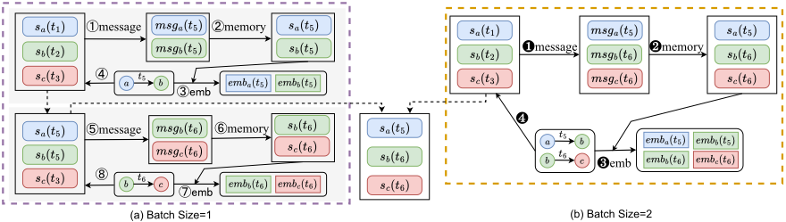
The ideal training process for MTGNN involves sequentially processing each edge event in chronological order to maintain strict dependencies between events. Consider an example shown in Figure 1(a), where two events occur, i.e., nodes a and b interact at t5, and nodes b and c interact at t6. We first generate memory information for nodes a and b (①②), followed by generating embeddings for the event at timestamp t5 (③). Subsequently, the memory is updated based on the event (④). This process is then repeated for events occurring at timestamp t6 (⑤⑥⑦⑧). This sequential processing meticulously maintains dependencies between events, and incorporates the latest memory state from all previous events of the corresponding nodes in each event processing.
However, this sequential training processing is particularly slow and poses serious efficiency problems, so batch parallel training methods are commonly employed to improve training efficiency [Zhou et al., 2022; Zhou et al., 2023; Gao et al., 2024; Chen et al., 2023b; Sheng et al., 2024; Chen et al., 2021]. In this approach, multiple consecutive edge events are grouped into a batch and trained simultaneously and in parallel. For example, Figure 1(b) shows the bach parallel training process of the above two events. Similarly, the steps (❶❷❸❹) are processed to generate messages, memory, and embeddings, and update the memory based on these events. However, under the batch strategy, only the latest message for the same node is retained for subsequent updates, while messages from other events are dropped. This difference leads to the memory staleness issue due to the inability to update the memory as in the ideal sequential processing (④), and finally results in degraded training accuracy.
2.3 Existing Efforts and Remaining Limitations
Several efforts have been made to address the memory staleness issue caused by batch training methods, including measuring memory loss to optimize data batch allocations [Gao et al., 2024; Lampert et al., 2024], overlapping batch training to capture missed events [Chen et al., 2023a; Zhou et al., 2022; Chen et al., 2023b], and introducing new memory compensation modules [Chen et al., 2021; Zhou et al., 2023; Zhang et al., 2023; Sheng et al., 2024; Su et al., 2024]. Despite these efforts, some limitations remain:
Limitation#1: Inaccurate measurement of coarse-grained memory loss. When nodes are repeated in a batch, it can lead to imprecise generation of memory and embedding due to staleness. The existing approach in state-of-the-art work ETC [Gao et al., 2024] calculates the number of repeated nodes within a batch to measure this intra-batch information loss. However, simply counting repeated nodes does not accurately capture the true memory loss, as missed information can impact messages, memory states, time embeddings, and other aspects. This approach overlooks the influence of memory aging nodes resulting from connectivity relationships and the evolving dynamic graph on changes in memory loss over time. For example, as shown in Figure 5, different times introduce varying levels of staleness. The imprecise measurement of coarse-grained memory loss results in inefficient batch allocation, hindering improving training efficiency.
Limitation#2: Trade-off in accuracy and efficiency for batch splitting. Guiding batch splitting based on memory loss measurement presents a challenge in balancing training efficiency and memory staleness. TGL [Zhou et al., 2022] uses a random batch scheduling strategy to enable crosstraining batches between epochs, but it only compensates for the number of times the final information is captured and does not fully resolve memory staleness. NeutronStream [Chen et al., 2023a] adopts a sliding window training method, adjusting adaptively to the longest window length without dependencies, but this introduces significant computational overhead. ETC [Gao et al., 2024] introduces a trade-off batch split strategy that prioritizes minimizing loss within each batch. Specifically, by setting the maximum value of pre-generated batches as a threshold, ETC allows batches with predicted memory loss below this threshold to increase in size. However, this strategy overlooks the overall impact of cumulative memory staleness across all batches.
Limitation#3: Limited capacity in memory compensation. To implement a memory compensation strategy, TIGER [Zhang et al., 2023] improves precision with dual memory modules but at the cost of high computational and storage overhead. In contrast, DistTGL [Zhou et al., 2023] and MSPipe [Sheng et al., 2024] focus on performance optimization, neglecting accuracy compensation and adding preprocessing computational expenses. Conversely, EDGE [Chen et al., 2021] disregards accuracy considerations in memory modules altogether. Moreover, current lightweight general correction strategies overlook explicit temporal encoding information. PRES [Su et al., 2024] utilizes an iterative prediction-correction scheme to continually correct information loss in memory:
where δsi represents the predictive model for correction, and γ is a learnable variable that balances the prediction and current memory state. However, this method computes predicted values for all nodes at each iteration, which may be impractical for dynamic graphs with a large number of nodes.
3 Methodology
3.1 Observations and Overview
We identify three key observations that affect memory staleness during batch parallel training. Using node b in Figure 1 as an example, we illustrate specific differences in Figure 2.
Observation#1: Lack of update times for memory states leads to memory staleness. In sequential training (batch=1), the learnable function mem(·) related to ⑥ is updated. However, in batch parallel training (batch size=2), the mem(·) function ❷ is not updated for the t6 event.
Observation#2: Inaccurate time embeddings also impact memory staleness. When utilizing batch parallel training, the time difference ∆t varies for different batch sizes, leading to inaccuracies in stale memory. For instance, the calculation of msgb(t6) involves the following time differences:
where ∆t is for batch size=1 and ∆t′ is for batch size=2.
Observation#3: Stale memory leads to stale messages from both source and target nodes. The message calculation connects the source node to the target node. Therefore, for an event at time t6, if the memory sb(t-) is outdated, this staleness will be transmitted to msgb(t) and msgc(t).
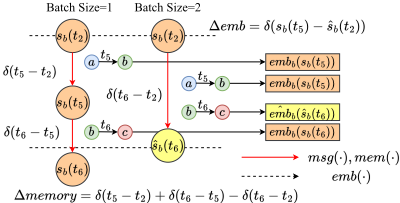
Based on our observations, we first propose a fine-grained memory loss measurement method that comprehensively evaluates information loss by considering node repetition frequency and timestamps. Additionally, we introduce an information-aware splitting strategy to minimize information loss by setting thresholds based on dynamic graph information and loss scores from training batches. We also present an optimized memory compensation strategy that corrects time encoding, adapts to batch strategy corrections, and adjusts to changes in batch sizes while incorporating temporal information. By integrating these strategies, we implement RBT, which ensures information integrity for balanced efficiency and accuracy. We will detail these three techniques next.
3.2 Fine-GrainedMemory Loss Measurement
Information loss. We propose a strategy to assess the loss caused by batch training. The loss of memory information encompasses memory loss, message loss, and the count of missing memory updates as indicated in Equation 2. In contrast to prior methodologies that primarily focus on the total count of loss events within a single batch [Gao et al., 2024], we assess the impact of including each event in the current batch separately. Let β(·) denote the score of information loss:
where Bi is the events set that assigned to i-th batch and β(Ek,Bi) represents the information loss score of a single event Ek that assigned to Bi. β(Bi) can be formulated as the sum of the information loss scores of all events assigned to the i-th batch. β(Ek, Bi) can be formulated as:
where β(Ek,Bi) is driven by memory loss (Lmem(·)), message loss (Lmsg(·)), and the count of missing memory update times (C(·)). Figure 3 illustrates how staleness is generated. Next, we will discuss the equation in detail for the memory loss, message loss and the count of missing memory updates.
Memory loss. We introduce the memory loss score of an event node within a batch. Let xk be an endpoint in the k-th event in batch i. It contributed to batch memory loss if and only if xk has appeared in a previous event.
where α(t) represents the set of events within i-th batch.
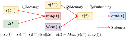
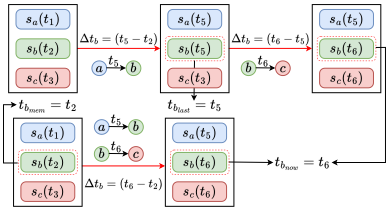
For memory loss (Lmem(·)) of Ek ∈ Bi (the k-th event of Bi), if the source node vsk or target node vdk have already occurred before, we use it as a measure of memory loss:
Message loss. For message loss (Lmsg(·)), which consists of three parts: the memory loss of the source and target nodes, and the loss caused by the time difference. Since the message passes between the source and target nodes, for nodes that have already occurred, the information loss is calculated once for each source and target. However, the message does not directly cause information loss, so we have halved the impact of this loss. For information loss due to time difference, we use cos(·) corresponding time encoding function:
The explanation of the time difference is shown in Figure 4. We take the event at time t6 of node b as an example. tbmem indicates the stale time of memory storage when using batch strategy. tblast indicates the ideal time of node b without batch strategy. tbnow is the time of the current event. Using the time difference equation, we can measure the difference between the ideal time and the actual time.
Missing update times. We amplify the information loss score according to the number of missing memory updates (C(·)) using ln(·). Generally, more repeats of nodes present in the current batch, more information loss is generated:
This fine-grained memory loss measurement considers factors like errors in time difference, previous memory state, and the impact of the learnable function, denoted by Lmsg, Lmem, and C. Specifically, Lmsg is influenced by both the previous memory state and time difference, Lmem is affected by the previous memory state alone, and C is impacted by the update frequency of the learnable function. Errors in the previous memory state directly worsen staleness in memory retention, affecting both Lmsg and Lmem.
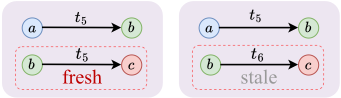
Besides, staleness is avoided for repeated nodes within a batch when they share the same timestamp, as demonstrated in Figure 5. In dynamic graphs with numerous identical timestamps, it is recommended to batch events occurring simultaneously for the same node to prevent information leakage. Exploring techniques to merge events with identical timestamps into a single batch while maintaining event dependencies offers a promising research direction.
3.3 Information Loss-aware Batch Splitting
Since some batches will inevitably experience significant information loss, we can improve system efficiency by ensuring that the loss value of all batches does not exceed a certain threshold while keeping the loss within each batch within an acceptable range. We believe that the information on the entire loss list and the entire dataset should be considered in a comprehensive way. Our equation is as follows:
where Lℓ represents the calculated loss list, n represents the number of nodes, and e represents the number of events, mean(Lℓ) represents the information loss value considering the entire loss list, while the latter half is an extension of the threshold value based on the repetition rate of the entire dynamic graph. For dynamic graphs with higher repetition rates, we allow a larger threshold, whereas for dynamic graphs with low repetition rates, a larger threshold is unacceptable.
3.4 OptimizedMemory Compensation
The previous correction strategy used all nodes for correction and only implied time information. This is inefficient not only on large-scale graphs, but also fails to characterize time changes in greater detail. Our time encoding correction strategy adapts to the batch training pattern and improves the ability to capture temporal information, which strengthens the expression ability of the correction model without significantly increasing the complexity of the model, we use ψ(·) to represent the temporal correction model:
where ψ(∆t) actually represents a time difference encoder adapted from a positional encoder of transformer:
Equation 13 indicates that the model can perceive the time difference information. Equation 14 shows our time difference encoder. We explicitly encode temporal information by using time differences where the original location is embedded. We do not use the time encoding used in msg(·), because we believe that implicit time coding has taken its current form and that by changing the way explicit time coding is performed, other potential information may be captured.
4 Experiment
4.1 Experiment Setups
Test Setup. Experiments are executed on Ubuntu 22.04.3 LTS machine, utilizing an Intel Xeon Gold 6342 CPU @2.80GHz and a Nvidia A40 48GB GPU, equipped with 1TB of memory and 40TB of disk space.
Datasets. We employ seven dynamic graph datasets: Wikipedia, Reddit, MOOC, LastFM (from JODIE [Kumar et al., 2019]), Flights (a flight traffic network [Poursafaei et al., 2022]), and user interaction data from WikiTalk [Leskovec, 2023b] and StackOverflow [Leskovec, 2023a]. Details are described in the appendix. The data partitioning followed a 70%-15%-15% split for training, validation, and testing, respectively, in line with previous studies [da Xu et al., 2020; Rossi et al., 2020; Gao et al., 2024; Li et al., 2023]. The specific information of each dataset is shown in Table 1.
Baselines. To evaluate the effectiveness of RBT, we compare it with the original TGL and the state-of-the-art ETC. To evaluate the impact of the batch strategy on efficiency and accuracy, we ensure consistency by using the same deredundancy and inter-batch pipelines across these baselines.
Parameter Configurations. The batch sizes are set to 600 and 1000 for testing, while other settings remain at their default values. Each dataset is trained for five epochs with five repetitions, and the mean of the final results is taken.
4.2 Main Results
We first provide an overall comparison between RBT and baselines, the results are summarized in Table 2. For small datasets like Wikipedia, Reddit, and MOOC, RBT performs a slight improvement upon TGL and ETC. Due to the relatively small scale of these datasets, the accuracy advantages of RBT were not fully evident, but RBT significantly boost computational efficiency while maintaining accuracy. In larger dataset like LastFM, RBT shows the most significant accuracy improvement. With a batch size of 1000, RBT boosts precision by around 3% compared to the higher-accuracy TGL method and approximately 5% compared to ETC. Even with a smaller batch size of 600, there is still a 2-3% accuracy enhancement, highlighting the effectiveness of RBT. RBT may not achieve optimal results in datasets with high frequencies of identical timestamps, such as Flights, where it could introduce noise and impede performance. However, in more general datasets with lower occurrences of identical timestamps, RBT's memory compensation strategy is effective in enhancing performance. While WikiTalk and StackOverflow datasets do not exhibit exceptional acceleration due to their large scale, there is still a notable efficiency enhancement.
| Dataset | src | dst | |V | | |E| |
|---|---|---|---|---|
| Wikipedia | 8,227 | 1,000 | 9,227 | 157,474 |
| 10,000 | 984 | 10,984 | 672,447 | |
| MOOC | 7,047 | 97 | 7,047 | 411,749 |
| LastFM | 980 | 1,000 | 1,980 | 1,293,103 |
| Flights | 11,574 | 12,939 | 13,169 | 1,927,145 |
| WikiTalk | 251,153 | 1,120,716 | 1,140,149 | 7,833,139 |
| StackOverflow | 2,226,243 | 2,296,666 | 2,601,977 | 63,497,049 |
| (%) | Wikipedia | MOOC | LastFM | Flights | WikiTalk | StackOverflow | ||||||||
|---|---|---|---|---|---|---|---|---|---|---|---|---|---|---|
| batch size:1000 | AP | AUC | AP | AUC | AP | AUC | AP | AUC | AP | AUC | AP | AUC | AP | AUC |
| TGL | 96.78 | 96.86 | 99.32 | 99.47 | 99.1 | 99.51 | 81.35 | 83.72 | 90.94 | 91.93 | 89.65 | 87.88 | 91.24 | 88.19 |
| ETC | 96.75 | 96.81 | 99.32 | 99.47 | 99.01 | 99.48 | 79.29 | 81.55 | 89.52 | 90.7 | 90.14 | 88.74 | 91.09 | 88.01 |
| RBT | 97.24 | 97.42 | 99.38 | 99.54 | 99 | 99.48 | 84.54 | 86.23 | 90.05 | 91.37 | 90.49 | 88.88 | 91.02 | 88.37 |
| batch size:600 | AP | AUC | AP | AUC | AP | AUC | AP | AUC | AP | AUC | AP | AUC | AP | AUC |
| TGL | 97.61 | 97.85 | 99.37 | 99.51 | 99.36 | 99.6 | 82.46 | 84.73 | 90.89 | 92.34 | 87.34 | 85.5 | 90.02 | 87.11 |
| ETC | 97.7 | 97.96 | 99.48 | 99.59 | 99.36 | 99.61 | 83.3 | 85.37 | 90.89 | 91.95 | 90.79 | 89.35 | 90.94 | 88.1 |
| RBT | 97.8 | 98.02 | 99.48 | 99.61 | 99.35 | 99.6 | 85.24 | 86.91 | 90.01 | 91.32 | 89.6 | 87.91 | 92.46 | 90.29 |
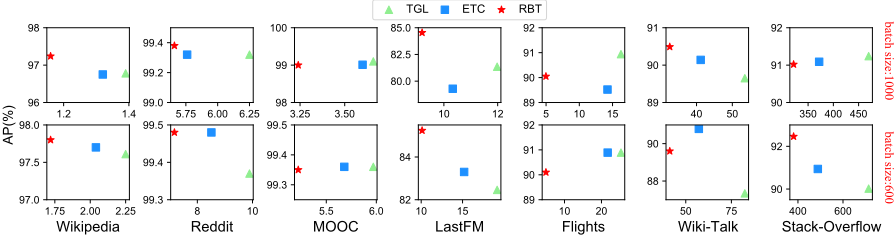
We also show the relationship between AP and time per epoch in Figure 6. In both the 1000 and 600 batch sizes, the RBT method significantly improves efficiency. Regardless of the dataset, the RBT method always achieves the fastest speed while ensuring the accuracy of the model. The speed gains are particularly noticeable on the Flights dataset. This substantial improvement is due to the fact that the timestamps in the Flights dataset represent days and that there are many flights departing at the same time on the same day. Using the RBT method to group a large number of events from the same day into the same batch, the efficiency is greatly enhanced without causing significant fluctuations in accuracy. In addition, we record the time proportion of correction strategies in the entire training at a batch size of 1000, as shown in Table 3. The time cost of correction only accounts for a small part, which is completely acceptable.
| RBT | Wikipedia Reddit MOOC LastFM Flights WikiTalk StackOverflow | ||||||
|---|---|---|---|---|---|---|---|
| C/T | 9% | 9% | 10% | 12% | 11% | 9% | 8% |
| Correction | 0.11 | 0.52 | 0.31 | 1.05 | 0.53 | 2.81 | 26.85 |
| Total | 1.16 | 5.66 | 3.24 | 9.19 | 4.98 | 32.52 | 321.34 |
4.3 Ablation Experiment
In this section, we use ablation experiments to demonstrate the effectiveness of our module. We set up two contrasts, using the PRES correction and without correction on batch sizes of 1000 and 600, to validate the effectiveness of our time encoding correction strategy, the results are shown in Table 4.
In Wikipedia, Reddit, MOOC, and LastFM datasets, our time encoding correction strategy achieved improvements in accuracy. Our correction strategy did not work for the Flights dataset, possibly because the Flights dataset has a large number of events with the same timestamp, making it difficult to capture explicit time changes. We will present a complete table in the appendix. Due to space constraints, we only present time comparisons of ablation experiments performed on the WikiTalk and StackOverflow datasets. For small data sets, the correction strategy has a lower overhead, so it can be directly selected to enable. The corresponding time comparison results are shown in Table 5.
Considering both the effectiveness and efficiency of WikiTalk and StackOverflow datasets in Table 4 and Table 5, we think that for large datasets, the time encoding correction strategy becomes less effective. Firstly, the graphs are too large, and explicit temporal information is difficult to capture effectively. Although the strategy may improve accuracy, the performance overhead introduced by the correction module outweighs its benefits. Therefore, for large datasets, a version without the correction strategy may be a better choice.
4.4 Batch Split Analysis
In this section, we use the LastFM dataset as an example to analyze the impact of our batch strategy on accuracy. We set the batch size to range from 1000 to 5000, with a step size of 500, and calculate the average batch size based on our partitioning strategy. The calculated average batch size is then used as the input for the TGL model, ensuring consistency with the batch size in our RBT method. Table 6 presents the corresponding batch sizes and their associated data.
| (%) | Wikipedia | MOOC | LastFM | Flights | WikiTalk | StackOverflow | ||||||||
|---|---|---|---|---|---|---|---|---|---|---|---|---|---|---|
| batch size:1000 | AP | AUC | AP | AUC | AP | AUC | AP | AUC | AP | AUC | AP | AUC | AP | AUC |
| RBT w/o PRES | 96.28 | 96.29 | 99.3 | 99.45 | 98.84 | 99.43 | 83.04 | 84.96 | 89.86 | 91.18 | 90.79 | 89.72 | 91.08 | 87.9 |
| RBT w/ PRES | 96.63 | 96.65 | 99.31 | 99.47 | 98.85 | 99.44 | 82.51 | 84.33 | 90.19 | 91.4 | 89.77 | 87.92 | 89.43 | 87.08 |
| RBT | 97.24 | 97.42 | 99.38 | 99.54 | 99 | 99.48 | 84.54 | 86.23 | 90.05 | 91.37 | 90.49 | 88.8 | 91.02 | 88.37 |
| batch size:600 | AP | AUC | AP | AUC | AP | AUC | AP | AUC | AP | AUC | AP | AUC | AP | AUC |
| RBT w/o PRES | 97.24 | 97.41 | 99.39 | 99.52 | 99.34 | 99.6 | 82.18 | 84.03 | 89.85 | 91.2 | 89.78 | 88.34 | 91.26 | 88.17 |
| RBT w/ PRES | 97.47 | 97.67 | 99.43 | 99.57 | 99.32 | 99.59 | 84.68 | 86.41 | 90.23 | 91.39 | 89.37 | 87.67 | 91.15 | 88.57 |
| RBT | 97.8 | 98.02 | 99.48 | 99.61 | 99.35 | 99.6 | 85.24 | 86.91 | 90.01 | 91.32 | 89.6 | 87.91 | 92.46 | 90.29 |
| w/o PRES w/ PRES RBT | w/o PRES w/ PRES | RBT | ||||
|---|---|---|---|---|---|---|
| Time(s) | batch size:1000 | batch size:600 | ||||
| WikiTalk | 29.15 | 32.01 | 32.52 | 37.67 | 40.09 | 41.23 |
| StackOverflow | 288.45 | 311.11 | 321.34 | 340.31 | 370.64 | 380.68 |
| Method | Batch size | ||||||||
|---|---|---|---|---|---|---|---|---|---|
| TGL | 1000 | 1500 | 2000 | 2500 | 3000 | 3500 | 4000 | 4500 | 5000 |
| RBT | 1810 | 2579 | 3187 | 3787 | 4595 | 5202 | 5878 | 6330 | 7184 |
After standardizing the batch size, we compare the TGL and RBT methods. To ensure fairness, it is important to note that we used the version without the calibration module, and the final results are shown in Figure 7(a). As shown in the figure, at each time step, the RBT method almost consistently maintains a higher accuracy level than the TGL method. This indicates that, even with the same average batch size, our method performs better in batch division on LastFM compared to traditional approaches, demonstrating that the RBT method effectively reduces memory loss within the batch. The TGL results reveal that a larger batch size may not always lead to a lower AP score due to internal memory staleness, impacting performance. In contrast, RBT uses a batch re-partitioning method to adjust batch sizes while maintaining consistent memory loss between batches, resulting in stable memory staleness and smoother curves. This highlights the difference in memory stability between RBT and TGL, with the latter showing more pronounced fluctuations in the curve.
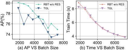
In addition, the main purpose of showing Figure 7(b) is to illustrate that, although the RBT method effectively constrains memory loss within the batch, it still cannot address the inherent issue in MTGNN training - that overly large batches remain difficult to train. This is an inherent limitation of the TGNN architecture, which is orthogonal to the RBT method.
5 RelatedWorks
To address the issue of memory staleness, certain techniques [Gao et al., 2024; Lampert et al., 2024] focus on measuring memory loss and adjusting data batch assignments by limiting the information loss per batch prevent performance degradation. ETC [Gao et al., 2024] sets a threshold on missed events per batch. LFIL [Lampert et al., 2024] uses a time window-based method to reduce time biases.Other techniques use overlapping batch training to capture missed events in previous batches and reduce memory staleness. NeutronStream [Chen et al., 2023a] employs sliding window training to capture cross-batch dependencies. TGL [Zhou et al., 2022] and SPEED [Chen et al., 2023b] partition training edges and randomly select chunks as the starting point, enabling the capture of large-scale events missed during different training iterations. Additionally, some techniques [Chen et al., 2021; Zhou et al., 2023; Zhang et al., 2023; Sheng et al., 2024; Su et al., 2024] enhance MTGNN's structure by introducing new modules or mechanisms to improve its ability to capture time information. EDGE [Chen et al., 2021] and DistTGL [Zhou et al., 2023] combine static and dynamic node memory to address latency. Meanwhile, TIGER [Zhang et al., 2023] and MSPipe [Sheng et al., 2024] use neighborhood information to minimize memory obsolescence. Moreover, PRES [Su et al., 2024] proposes an iterative predictive correction scheme with memory coherent learning objectives.
6 Conclusion
This paper introduces RBT, a methodology for dynamic graph learning that minimizes information loss in batch training. It utilizes a refined memory loss metric to measure memory staleness and adjusts batch splitting strategy to keep information loss within acceptable levels in each batch. Additionally, to balance efficiency and accuracy, an effective compensation mechanism is proposed to enhance memory precision. Experimental results show efficiency gains while preserving stable accuracy. A promising future direction is to explore batch reordering for large-scale dynamic graphs with the same timestamp, potentially reducing event dependencies without violating the temporal order.
Acknowledgments
This research is supported by the "Pioneer" R&D Program of Zhejiang (Grant No.2024C01019), the Starry Night Science Fund of Zhejiang University Shanghai Institute for Advanced Study (Grant No.SN-ZJU-SIAS-001), the Hangzhou Joint Fund of the Zhejiang Provincial Natural Science Foundation of China (Grant No.LHZSD24F020001), and the National Natural Science Foundation of China (Grant No.62476238). We gratefully acknowledges the support of Zhejiang University Education Foundation Qizhen Scholar Foundation.
@inproceedings{ijcai2025p312,
  title     = {Efficient Dynamic Graphs Learning with Refined Batch Parallel Training},
  author    = {Feng, Zhengzhao and Wang, Rui and Zhang, Longjiao and Zheng, Tongya and Huang, Ziqi and Song, Mingli},
  booktitle = {Proceedings of the Thirty-Fourth International Joint Conference on
               Artificial Intelligence, {IJCAI-25}},
  publisher = {International Joint Conferences on Artificial Intelligence Organization},
  editor    = {James Kwok},
  pages     = {2802--2810},
  year      = {2025},
  month     = {8},
  note      = {Main Track},
  doi       = {10.24963/ijcai.2025/312},
  url       = {https://doi.org/10.24963/ijcai.2025/312},
}
TY - CPAPER TI - Efficient Dynamic Graphs Learning with Refined Batch Parallel Training AU - Feng, Zhengzhao AU - Wang, Rui AU - Zhang, Longjiao AU - Zheng, Tongya AU - Huang, Ziqi AU - Song, Mingli T2 - Proceedings of the Thirty-Fourth International Joint Conference on Artificial Intelligence, IJCAI-25 PB - International Joint Conferences on Artificial Intelligence Organization PY - 2025 SP - 2802 EP - 2810 DO - 10.24963/ijcai.2025/312 UR - https://doi.org/10.24963/ijcai.2025/312 ER -Copied
Machine-readable versions of this paper, for tools and AI agents:





