
Prototype-based Optimal Transport for Out-of-Distribution Detection
Proceedings of the Thirty-Fourth International Joint Conference on Artificial Intelligence. Main Track. Pages 3018-3026.
https://doi.org/10.24963/ijcai.2025/336
Keywords
- Machine Learning: ML: Trustworthy machine learning
- Data Mining: DM: Anomaly/outlier detection
Abstract
Detecting Out-of-Distribution (OOD) inputs is crucial for improving the reliability of deep neural networks in the real-world deployment. In this paper, inspired by the inherent distribution shift between in-distribution (ID) and OOD data, we propose a novel method that leverages optimal transport to measure the distribution discrepancy between test inputs and ID prototypes. The resulting transport costs are used to quantify the individual contribution of each test input to the overall discrepancy, serving as a desirable measure for OOD detection. To address the issue that solely relying on the transport costs to ID prototypes is inadequate for identifying OOD inputs closer to ID data, we generate virtual outliers to approximate the OOD region via linear extrapolation. By combining the transport costs to ID prototypes with the costs to virtual outliers, the detection of OOD data near ID data is emphasized, thereby enhancing the distinction between ID and OOD inputs. Extensive evaluations demonstrate the superiority of our method over state-of-the-art methods.
- [Arjovsky et al., 2017] Martin Arjovsky, Soumith Chintala, and Leon Bottou. Wasserstein gan. In arXiv preprint arXiv:1701.07875, 2017.
- [Bendale and Boult, 2016] Abhijit Bendale and Terrance E. Boult. Towards open set deep networks. In CVPR, pages 1563-1572. IEEE, 2016.
- [Bitterwolf et al., 2023] Julian Bitterwolf, Maximilian Müller, and Matthias Hein. In or out? fixing imagenet out-of-distribution detection evaluation. In ICML, pages 2471-2506. PMLR, 2023.
- [Caron et al., 2020] Mathilde Caron, Ishan Misra, Julien Mairal, Priya Goyal, Piotr Bojanowski, and Armand Joulin. Unsupervised learning of visual features by con- trasting cluster assignments. NeurIPS, 33:9912-9924, 2020.
- [Cimpoi et al., 2014] Mircea Cimpoi, Subhransu Maji, Ia- sonas Kokkinos, Sammy Mohamed, and Andrea Vedaldi. Describing textures in the wild. In CVPR, pages 3606- 3613. IEEE, 2014.
- [Cuturi, 2013] Marco Cuturi. Sinkhorn distances: Light- speed computation of optimal transport. NeurIPS, 26, 2013.
- [Deng, 2012] Li Deng. The mnist database of handwritten digit images for machine learning research [best of the web]. IEEE Signal Processing Magazine, 29(6):141-142, 2012.
- [DeVries and Taylor, 2018] Terrance DeVries and Gra- ham W. Taylor. Learning confidence for out-of- distribution detection in neural networks. arXiv preprint arXiv:1802.04865, 2018.
- [Djurisic et al., 2023] Andrija Djurisic, Nebojsa Bozanic, Arjun Ashok, and Rosanne Liu. Extremely simple acti- vation shaping for out-of-distribution detection. In ICLR, 2023.
- [Dosovitskiy and et al, 2021] Alexey Dosovitskiy and Lu- cas Beyer et al. An image is worth 16x16 words: Trans- formers for image recognition at scale. In ICLR, 2021.
- [Filos et al., 2020] Angelos Filos, Panagiotis Tigkas, Rowan McAllister, Nicholas Rhinehart, Sergey Levine, and Yarin Gal. Can autonomous vehicles identify, recover from, and adapt to distribution shifts? In ICML, pages 3145-3153.
- PMLR, 2020.
- [Garg et al., 2023] Sahil Garg, Sanghamitra Dutta, Mina Dalirrooyfard, Anderson Schneider, and Yuriy Nevmy- vaka. In-or out-of-distribution detection via dual diver- gence estimation. In Uncertainty in Artificial Intelligence, pages 635-646. PMLR, 2023.
- [Ge et al., 2021] Zheng Ge, Songtao Liu, Zeming Li, Osamu Yoshie, and Jian Sun. Ota: Optimal transport assignment for object detection. In CVPR, pages 303-312, 2021.
- [He et al., 2016] Kaiming He, Xiangyu Zhang, Shaoqing Ren, and Jian Sun. Deep residual learning for image recog- nition. In CVPR, pages 770-778. IEEE, 2016.
- [Hendrycks and Gimpel, 2017] Dan Hendrycks and Kevin Gimpel. A baseline for detecting misclassified and out-of- distribution examples in neural networks. In ICLR, 2017.
- [Hendrycks et al., 2019a] Dan Hendrycks, Mantas Mazeika, and Thomas Dietterich. Deep anomaly detection with out- lier exposure. In ICLR, 2019.
- [Hendrycks et al., 2019b] Dan Hendrycks, Mantas Mazeika, Saurav Kadavath, and Dawn Song. Using self-supervised learning can improve model robustness and uncertainty. In NeurIPS, pages 15637-15648, 2019.
- [Hendrycks et al., 2022] Dan Hendrycks, Steven Basart, Mantas Mazeika, Andy Zou, Joseph Kwon, Moham- madreza Mostajabi, Jacob Steinhardt, and Dawn Song. Scaling out-of-distribution detection for real-world set- tings. In ICML, pages 8759-8773. PMLR, 2022.
- [Horn et al., 2018] Grant Van Horn, Oisin Mac Aodha, Yang Song, Yin Cui, Chen Sun, Alexander Shepard, Hartwig Adam, Pietro Perona, and Serge J. Belongie. The inatural- ist species classification and detection dataset. In CVPR, pages 8769-8778. IEEE, 2018.
- [Hsu et al., 2020] Yen-Chang Hsu, Yilin Shen, Hongxia Jin, and Zsolt Kira. Generalized ODIN: detecting out-of-distribution image without learning from out-of- distribution data. In CVPR, pages 10948-10957. IEEE, 2020.
- [Huang et al., 2021] Rui Huang, Andrew Geng, and Yixuan Li. On the importance of gradients for detecting distribu- tional shifts in the wild. In NeurIPS, pages 677-689, 2021.
- [Krizhevsky, 2009] Alex Krizhevsky. Learning multiple lay- ers of features from tiny images. 2009.
- [Le and Yang, 2015] Ya Le and Xuan S. Yang. Tiny ima- genet visual recognition challenge. CS 231N, 7(7):3, 2015.
- [Lee et al., 2018] Kimin Lee, Kibok Lee, Honglak Lee, and Jinwoo Shin. A simple unified framework for detect- ing out-of-distribution samples and adversarial attacks. In NeurIPS, pages 7167-7177, 2018.
- [Liang et al., 2018] Shiyu Liang, Yixuan Li, and R. Srikant. Enhancing the reliability of out-of-distribution image de- tection in neural networks. In ICLR, 2018.
- [Liu et al., 2020] Weitang Liu, Xiaoyun Wang, John D. Owens, and Yixuan Li. Energy-based out-of-distribution detection. In NeurIPS, pages 21464-21475, 2020.
- [Liu et al., 2023] Xixi Liu, Yaroslava Lochman, and Christo- pher Zach. GEN: pushing the limits of softmax-based out- of-distribution detection. In CVPR, pages 23946-23955. IEEE, 2023.
- [Liu et al., 2024] Yibing Liu, Chris XING TIAN, Haoliang Li, Lei Ma, and Shiqi Wang. Neuron activation cover- age: Rethinking out-of-distribution detection and general- ization. In ICLR, 2024.
- [Lu et al., 2023] Fan Lu, Kai Zhu, Wei Zhai, Kecheng Zheng, and Yang Cao. Uncertainty-aware optimal trans- port for semantically coherent out-of-distribution detec- tion. In CVPR, pages 3282-3291, 2023.
- [Ming et al., 2022] Yifei Ming, Ying Fan, and Yixuan Li. Poem: Out-of-distribution detection with posterior sam- pling. In ICML, pages 15650-15665. PMLR, 2022.
- [Nalisnick et al., 2018] Eric Nalisnick, Akihiro Matsukawa, Yee Whye Teh, Dilan Gorur, and Balaji Lakshmi- narayanan. Do deep generative models know what they don't know? arXiv preprint arXiv:1810.09136, 2018.
- [Netzer et al., 2011] Yuval Netzer, Tao Wang, Adam Coates, Alessandro Bissacco, Bo Wu, and Andrew Y. Ng. Reading digits in natural images with unsupervised feature learn- ing. In NeurIPS Workshop, 2011.
- [Peyré et al., 2019] Gabriel Peyré, Marco Cuturi, et al. Com- putational optimal transport: With applications to data sci- ence. Foundations and Trends® in Machine Learning, 11(5-6):355-607, 2019.
- [Ren et al., 2021] Jie Ren, Stanislav Fort, Jeremiah Z. Liu, Abhijit Guha Roy, Shreyas Padhy, and Balaji Lak- shminarayanan. A simple fix to mahalanobis dis- tance for improving near-ood detection. arXiv preprint arXiv:2106.09022, 2021.
- [Sastry and Oore, 2020] Chandramouli Shama Sastry and Sageev Oore. Detecting out-of-distribution examples with gram matrices. In ICML, pages 8491-8501. PMLR, 2020.
- [Sehwag et al., 2021] Vikash Sehwag, Mung Chiang, and Prateek Mittal. SSD: A unified framework for self- supervised outlier detection. In ICLR, 2021.
- [Song et al., 2022] Yue Song, Nicu Sebe, and Wei Wang. Rankfeat: Rank-1 feature removal for out-of-distribution detection. In NeurIPS, 2022.
- [Sun and Li, 2022] Yiyou Sun and Yixuan Li. DICE: lever- aging sparsification for out-of-distribution detection. In ECCV, pages 691-708. Springer, 2022.
- [Sun et al., 2021] Yiyou Sun, Chuan Guo, and Yixuan Li. React: Out-of-distribution detection with rectified activa- tions. In NeurIPS, pages 144-157, 2021.
- [Sun et al., 2022] Yiyou Sun, Yifei Ming, Xiaojin Zhu, and Yixuan Li. Out-of-distribution detection with deep nearest neighbors. In ICML, pages 20827-20840. PMLR, 2022.
- [Tanwisuth et al., 2021] Korawat Tanwisuth, Xinjie Fan, Huangjie Zheng, Shujian Zhang, Hao Zhang, Bo Chen, and Mingyuan Zhou. A prototype-oriented framework for unsupervised domain adaptation. NeurIPS, 34:17194- 17208, 2021.
- [Turrisi et al., 2022] Rosanna Turrisi, Rémi Flamary, Alain Rakotomamonjy, and Massimiliano Pontil. Multi-source domain adaptation via weighted joint distributions optimal transport. In Uncertainty in Artificial Intelligence, pages 1970-1980. PMLR, 2022.
- [Vaze et al., 2022] Sagar Vaze, Kai Han, Andrea Vedaldi, and Andrew Zisserman. Open-set recognition: A good closed-set classifier is all you need. In ICLR, 2022.
- [Wang and Deng, 2021] Mei Wang and Weihong Deng. Deep face recognition: A survey. Neurocomputing, 429:215-244, 2021.
- [Wang et al., 2022a] Haobo Wang, Mingxuan Xia, Yixuan Li, Yuren Mao, Lei Feng, Gang Chen, and Junbo Zhao. Solar: Sinkhorn label refinery for imbalanced partial-label learning. NeurIPS, 2022.
- [Wang et al., 2022b] Haoqi Wang, Zhizhong Li, Litong Feng, and Wayne Zhang. Vim: Out-of-distribution with virtual-logit matching. In CVPR, pages 4911-4920. IEEE, 2022.
- [Wang et al., 2023] Qizhou Wang, Junjie Ye, Feng Liu, Quanyu Dai, Marcus Kalander, Tongliang Liu, Jianye Hao, and Bo Han. Out-of-distribution detection with implicit outlier transformation. In ICLR, 2023.
- [Zhang et al., 2023a] Jingyang Zhang, Nathan Inkawhich, Randolph Linderman, Yiran Chen, and Hai Li. Mixture outlier exposure: Towards out-of-distribution detection in fine-grained environments. In WACV, pages 5531-5540, 2023.
- [Zhang et al., 2023b] Jingyang Zhang, Jingkang Yang, Pengyun Wang, Haoqi Wang, Yueqian Lin, Haoran Zhang, Yiyou Sun, Xuefeng Du, Kaiyang Zhou, Wayne Zhang, Yixuan Li, Ziwei Liu, Yiran Chen, and Hai Li. Openood v1.5: Enhanced benchmark for out-of- distribution detection. arXiv preprint arXiv:2306.09301, 2023.
- [Zhang et al., 2023c] Jinsong Zhang, Qiang Fu, Xu Chen, Lun Du, Zelin Li, Gang Wang, Xiaoguang Liu, Shi Han, and Dongmei Zhang. Out-of-distribution detection based on in-distribution data patterns memorization with modern hopfield energy. In ICLR, 2023.
- [Zhou et al., 2018] Bolei Zhou, Àgata Lapedriza, Aditya Khosla, Aude Oliva, and Antonio Torralba. Places: A 10 million image database for scene recognition. PAMI, 40(6):1452-1464, 2018.
- [Zhu et al., 2023] Jianing Zhu, Yu Geng, Jiangchao Yao, Tongliang Liu, Gang Niu, Masashi Sugiyama, and Bo Han. Diversified outlier exposure for out- of-distribution detection via informative extrapolation. NeurIPS, 36:22702-22734, 2023.
References were extracted automatically from the PDF and may contain errors.
Full text extracted automatically from the PDF; figures, tables and equations may differ. The PDF is the version of record.
1 Introduction
Deep neural networks (DNNs) deployed in real-world scenarios often encounter out-of-distribution (OOD) inputs, such as inputs not belonging to one of the DNN's known classes. Ideally, reliable DNNs should be aware of what they do not know. However, they typically make overconfident predictions on OOD data [Nalisnick et al., 2018]. This notorious behavior undermines the credibility of DNNs and could pose risks to involved users, particularly in safety-critical applications like autonomous driving [Filos et al., 2020] and biometric authentication [Wang and Deng, 2021]. This gives rise to the importance of OOD detection, which identifies whether an input is OOD and enables conservative rejection or transferring decision-making to humans for better handling.
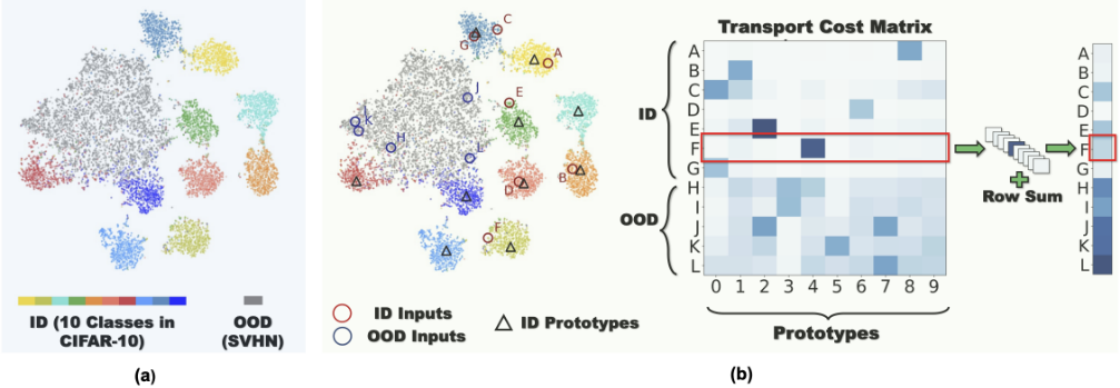
The representations of ID data within the same class tend to be gathered together after the training process, as shown in Figure 1(a). In contrast, the representations of OOD data are relatively far away from ID data, as they are not involved in the training process. In other words, the distributions of ID and OOD representations in the latent space exhibit a distinct separation. Therefore, we can expect that the distribution discrepancy between the representations of test inputs (i.e., a mixture of ID and OOD data) and pure ID data is primarily caused by the presence of OOD data. Such a distribution discrepancy motivates us to differentiate OOD data from test inputs by quantifying the individual contribution of each test input to the overall distribution discrepancy.
In this way, a critical question arises: how to measure the distribution discrepancy between test inputs and ID data, while quantifying the contribution of each test input? To this end, we utilize optimal transport (OT), a principled approach with rich geometric awareness for measuring the discrepancy between distributions. Concretely, OT aims to minimize the total transport cost between two distributions to measure the distribution discrepancy based on a predefined cost function (typically the geometric distance between samples). The smaller the total cost is, the closer the two distributions are. Since the total cost comprises the sum of transport costs between sample pairs, OT facilitates a fine-grained assessment of individual sample contributions to the overall discrepancy, making it particularly well-suited for OOD detection. Furthermore, the transport cost captures the geometric differences between ID and OOD representations in the latent space, providing a geometrically meaningful interpretation.
Based on the above intuition, in this paper, we propose a novel OOD detection method called POT that utilizes the Prototype-based Optimal Transport. Concretely, we first construct ID prototypes with the class-wise average of training sample representations to represent the distribution of ID data. We then apply OT between the representations of test inputs and the ID prototypes, obtaining a transport cost matrix where each entry indicates the transport cost between the corresponding pair of test input and prototype. As illustrated in Figure 1(b), the total transport cost, calculated by summing all matrix entries, reflects the overall distribution discrepancy. The transport cost from each test sample to all ID prototypes (i.e., the row sum), serves as a measure of individual contribution to the overall discrepancy, indicating the likelihood of being OOD. However, the task of OOD detection remains inadequately addressed due to the presence of OOD data with smaller distribution shifts. These OOD data lie closer to ID data in the latent space, rendering the transport costs to ID prototypes insufficient for detecting them. To tackle this issue, we propose generating virtual outliers to approximate the OOD region, particularly the areas near ID prototypes, using linear extrapolation between ID prototypes and the average representation of test inputs. By integrating the transport costs from test inputs to ID prototypes with the cost to virtual outliers, the detection of OOD samples with smaller distribution shifts could be emphasized, thereby enhancing the overall distinction between ID and OOD data.
Our key contributions are as follows: (1) We present a novel perspective for OOD detection by measuring distribution discrepancy and propose an effective detection method using prototype-based optimal transport. (2) Extensive experiments on various benchmark datasets demonstrate that our proposed method achieves state-of-the-art (SOTA) performance, outperforming 21 previous OOD detection methods. Moreover, in the scenarios where training data is unavailable, our method consistently beats the robust competitors by a margin of 22.5% in FPR95 on the CIFAR-100 benchmark.
2 RelatedWork
2.1 OODDetection
OOD detection has attracted growing research attention in recent years. Existing approaches can generally be categorized into two major lines:
(1) One line of work utilizes the outputs from pretrained models to design scoring functions for differentiating OOD samples. These post-hoc methods can be further divided into three subcategories. 1) The confidence-based methods [Sun et al., 2021; Song et al., 2022; Hendrycks et al., 2022; Wang et al., 2022b; Liu et al., 2023] adjusts model outputs to obtain the desired confidence, including maximum softmax probability [Hendrycks and Gimpel, 2017], energy [Liu et al., 2020], and generalized entropy [Liu et al., 2023]. 2) The density-based methods [Hendrycks et al., 2022; Sun and Li, 2022; Zhang et al., 2023c; Liu et al., 2024] identifies certain properties or patterns of ID data, such as neuron coverage [Liu et al., 2024], by learning the corresponding density functions, and the OOD samples that deviate from these properties or patterns tend to reside in low-density regions. 3) The distance-based methods [Lee et al., 2018; Ren et al., 2021; Sehwag et al., 2021; Sun et al., 2022] adopts distance metrics, e.g., Mahalanobis distance, between test input and ID samples or centroids differentiate OOD samples, under the assumption that OOD data lie relatively far away from ID data. Different from these works, we introduce a novel perspective for OOD detection on measuring distribution discrepancy. The most closely related work is dual divergence estimation (DDE) [Garg et al., 2023], which estimates the dual KL-Divergence between the test samples and ID samples. However, while DDE estimates divergence in a dual space optimized by DNNs and relies heavily on the quality of transformed sample representations, POT enables direct measurement of distribution discrepancy in the latent space.
(2) Another line of work focuses on altering models with training-time regularization to amplify the differences between OOD and ID samples [Hendrycks et al., 2019a; Ming et al., 2022; Zhang et al., 2023a; Wang et al., 2023; Lu et al., 2023]. For example, by incorporating a suitable loss, models are encouraged to produce predictions with uniform distributions [Hendrycks et al., 2019a] or higher energy [Liu et al., 2020] for OOD data. Building on this, some approaches investigate refining or synthesizing outliers to improve the model performance. For instance, [Ming et al., 2022] utilizes a posterior sampling-based technique to select the most informative OOD samples from a large outlier set, while [Wang et al., 2023] implicitly expands the auxiliary outliers by perturbing model parameters. However, the cost of model retraining can be prohibitive, especially when the parameter scale is large. Additionally, modifying models may also have side effects of degrading model performance on the original task. In contrast, this paper focus on post-hoc methods, which are easy to implement and generally applicable across different models. Such properties are highly practical for adopting OOD detection methods in real-world applications.
2.2 Optimal Transport
As a mathematical tool for comparing distributions, optimal transport (OT) has been successfully employed in diverse machine learning tasks, including domain adaptation [Turrisi et al., 2022], generative adversarial training [Arjovsky et al., 2017], object detection [Ge et al., 2021], and partial-label learning [Wang et al., 2022a]. The most related one to our work is [Lu et al., 2023], which also applies OT for the OOD detection problem. By assuming both an unlabeled and a labeled training set, [Lu et al., 2023] uses OT to guide the clustering of samples for label assignment to the unlabeled samples, thereby augmenting the training data and facilitating the model retraining for OOD detection. In contrast, our work operates in a post-hoc manner without the requirement of extra training data or model retraining.
3 The ProposedMethod
3.1 Problem Setting
In the context of supervised multi-class classification, we denote the data space as X and the corresponding label space as Y = {1, 2, · · · , C}. The training dataset with in-distribution (ID) samples Dtr = {(xi, yi)}ni=1 is sampled from the joint distribution PXY. The marginal distribution on X is denoted as P in X . The model trained on training data typically consists of a feature encoder g : X → Rd , mapping the input x ∈ X to a d-dimensional representation, and a linear classification layer f : Rd → RC , producing a logit vector containing classification confidence for each class. Given the test inputs Dte = {xj}mj=1 , the goal of OOD detection is to identify whether xj is out-of-distribution w.r.t P in X .
3.2 Prototype-based Optimal Transport for OOD Detection
Constructing Class Prototypes The key idea of our method is to use OT to measure the distribution discrepancy between test inputs and ID data while quantifying the individual contribution of each test input. A straightforward approach involves applying OT between test inputs and the training data. However, the standard OT is essentially a linear programming problem, suffering from cubic time complexity and incurring prohibitive computational cost when applied to largescale training sets [Peyr´e et al., 2019]. An alternative is to sample a smaller subset of the training set for efficiency, but this can result in missing classes, leading to mismatches in ID inputs. Such mismatches can exaggerate the contribution of ID inputs to the distribution discrepancy, thus incorrectly identifying them as OOD. To overcome this, we propose to characterize each class with a prototype and align test inputs to these prototypes. Specifically, given the training dataset Dtr = {(xi, yi)}ni=1 , we construct prototype for each class as the average representation for that class extracted from the feature encoder g:
where Nc is the number of samples in class c. The utilization of prototypes offers two key benefits: it reduces computational overhead by reducing the data scale and ensures all classes are represented, mitigating the risk of mismatches caused by missing classes.
OOD Detection Using Prototype-based Optimal Transport By formalizing an optimal transport problem between the representations of test inputs {zj = g(xj)}mj=1 and ID prototypes {ηi}Ci=1 , we search for the minimal transport cost that represents the distribution discrepancy, while subject to the mass conservation constraint:
where ⟨·, ·⟩F stands for the Frobenius dot-product. µ and ν are the probability simplexes of ID prototypes and test samples:
where pi = Ni ∑ni=1 Ni , qj = 1m , and δηi is the Dirac at position ηi. γ is a transport plan, essentially a joint probability matrix, with an entry γij describing the amount of probability mass transported from prototype ηi to test input zj. All feasible transport plans constitute the transportation polytope Π(µ, ν) [Cuturi, 2013]. E is the ground cost matrix, where the entry Eij denotes the point-to-point moving cost between ηi and zj, which is defined with the Euclidean distance as Eij = ||ηi - zj ||2.
To efficiently resolve Equation 2, we introduce the entropic regularization term H(γ) and write the optimization problem as:
where λ > 0 and H(γ) = ∑i,j γij(log γij - 1) [Peyr´e et al., 2019]. In this way, the optimal transport plan γ can be written as:
Here, a ∈ RC and b ∈ Rm are known as scaling variables. This formulation can be solved much faster using the Sinkhorn-Knopp algorithm [Cuturi, 2013]:
(6)
where ⊘ denotes element-wise division. Detailed derivations are provided in Appendix 6.1. With the λ-strong convexity [Peyr´e et al., 2019], the entropic regularized OT could be solved in quadratic time complexity O(nm), where n and m denote the number of data points in the two distributions,
respectively. Since the ID distribution is represented with a fixed number of prototypes, the prototype-based OT has linear time complexity O(Cm).
To evaluate whether an input sample xj ∈ Dte is OOD or not, we derive the cost of moving it to all ID prototypes Tj by decomposing the total transport cost:
As the total transport cost serves as a measure of distributional discrepancy between ID and test data, a higher transport cost T for a test sample indicates a greater deviation from the ID data, suggesting the sample is more likely to be OOD. We emphasize that, while the solution of OT is the transport plan γ, which is often the focus in many applications [Caron et al., 2020; Wang et al., 2022a], our concentration lies on the transport costs between sample pairs. Specifically, it is the product of transport plan and ground cost, serving as a desirable and interpretable measure for OOD detection.
Data Augmentation via Linear Extrapolation As described above, the transport cost can serve as a measure for OOD detection. However, relying solely on the cost to ID prototypes is insufficient for discerning OOD data with smaller distribution shifts from ID data. It is because such OOD data are located closer to ID data in the latent space and tend to incur lower transport costs to ID prototypes. Meanwhile, the mass conservation constraint inherent in OT may exacerbate this issue by enforcing transportation between OOD data and prototypes when ID inputs are sparse. To address this issue, we propose to generate virtual outliers to approximate the OOD region using linear extrapolation. By integrating the transport costs from test inputs to both virtual outliers and ID prototypes, we introduce a contrastive transport cost, which enhances the detection performance, particularly for the OOD inputs with smaller distribution shifts.
Given two representations zi and zj, the linear extrapolation between them is defined as:
Instead of generating outliers aimlessly by enumerating available sample pairs, we construct virtual outliers P ∗ by combining the prototypes P and the average of test inputsM:
where ω > 1 ensures that the generated points P ∗ lies beyond M. The underlying intuition is that M can be expressed as a linear interpolation of the average representations of test ID samples Min and test OOD samples Mout:

where Nin and Nout denote the number of test ID samples and total test samples, respectively. As illustrated in Figure 2, the point M resides between ID and OOD data, guiding the direction for outlier generation in response to distribution shifts. As parameter ω increases, the generated virtual outliers progressively move away from the ID prototypes towards the OOD region in the latent space. By choosing an appropriate parameter, we can control the location of generated virtual outliers to emphasize the detection of OOD inputs with smaller distributions shifts. In contrast to the method [Zhu et al., 2023] that conducts informative extrapolation to synthesize numerous outliers during training with assumed auxiliary outliers, the linear extrapolation is a lightweight operation that does not require training or auxiliary outliers.
Likewise, after generating the virtual outliers P ∗ , we apply the entropic regularized OT between P ∗ and the test inputs to obtain the corresponding transport cost T ∗ . By taking the difference of transport costs from test inputs to the ID prototypes and to the virtual outliers, we derive the contrastive transport cost T -T ∗ as the final OOD score. Given the opposite trends of T and T ∗ in indicating whether a sample is ID or OOD, a higher contrastive transport cost denotes a higher likelihood of the test input being OOD.
4 Experiments
In this section, we preform extensive experiments over OOD detection benchmarks. All the experimental setup adheres to the latest version of OpenOOD, an open repository for benchmarking generalized OOD detection 1 [Zhang et al., 2023b].
4.1 Common Setup
Datasets We assess the performance of our proposed POT on the widely used CIFAR-100 benchmark and ImageNet1k benchmark, which regard CIFAR-100 and ImageNet1k as ID datasets, respectively. For CIFAR-100, we use the standard split, with 50,000 training images and 10,000 test images. For ImageNet-1k, we utilize 50,000 images from the validation set as ID test set. For each benchmark, OpenOOD splits OOD data to Far-OOD and NearOOD based on their degrees of the semantic similarity with ID data. Specifically, the CIFAR-100 benchmark utilizes four Far-OOD datasets: MNIST [Deng, 2012], SVHN [Netzer et al., 2011], Textures [Cimpoi et al., 2014], and Places365 [Zhou et al., 2018], along with two Near-OOD datasets: CIFAR-10 and Tiny Imagenet [Le and Yang, 2015]. For the large-scale ImageNet-1k benchmark, it considers iNaturalist [Horn et al., 2018], Textures [Cimpoi et al., 2014], and OpenImage-O [Wang et al., 2022b] as Far-OOD datasets. In terms of Near-OOD datasets, SSB-hard [Vaze et al., 2022] and NINCO [Bitterwolf et al., 2023] are included.
1 https://github.com/Jingkang50/OpenOOD
| Method | MINIST | SVHN | Textures | Places365 | Average | |||||
|---|---|---|---|---|---|---|---|---|---|---|
| FPR95↓ | AUROC↑ | FPR95↓ | AUROC↑ | FPR95↓ | AUROC↑ | FPR95↓ | AUROC↑ | FPR95↓ | AUROC↑ | |
| OpenMax | 53.97±4.71 | 75.89±1.40 | 52.81±1.89 | 82.05±1.55 | 56.16±1.86 | 80.46±0.10 | 54.99±1.42 | 79.22±0.41 | 54.48±0.63 | 79.40±0.41 |
| MSP | 57.24±4.67 | 76.08±1.86 | 58.43±2.61 | 78.68±0.95 | 61.79±1.31 | 77.32±0.71 | 56.64±0.87 | 79.22±0.29 | 58.52±1.12 | 77.83±0.45 |
| ODIN | 45.93±3.24 | 83.79±1.30 | 67.21±3.95 | 74.72±0.77 | 62.39±2.87 | 79.34±1.08 | 59.73±0.86 | 79.45±0.25 | 58.81±0.78 | 79.32±0.22 |
| MDS | 71.70±2.89 | 67.47±0.81 | 67.72±6.05 | 70.20±6.52 | 70.55±2.50 | 76.23±0.69 | 79.57±0.34 | 63.17±0.50 | 72.38±1.53 | 69.27±1.41 |
| MDSEns | 2.86±0.85 | 98.20±0.78 | 82.57±2.57 | 53.74±1.62 | 84.91±0.87 | 69.75±1.14 | 96.58±0.19 | 42.32±0.74 | 66.73±1.05 | 66.00±0.69 |
| RMDS | 51.99±6.34 | 79.78±2.50 | 51.10±3.62 | 85.09±1.09 | 54.06±1.02 | 83.61±0.52 | 53.58±0.33 | 83.39±0.47 | 52.68±0.65 | 82.97±0.42 |
| Gram | 53.35±7.51 | 80.78±4.14 | 20.40±1.69 | 95.47±0.58 | 89.84±2.87 | 70.61±1.44 | 95.03±0.63 | 46.09±1.28 | 64.66±2.30 | 73.24±1.05 |
| EBO | 52.62±3.83 | 79.18±1.36 | 53.19±3.25 | 82.28±1.78 | 62.38±2.08 | 78.35±0.84 | 57.70±0.87 | 79.50±0.23 | 56.47±1.41 | 79.83±0.62 |
| GradNorm | 86.96±1.45 | 65.35±1.12 | 69.38±8.40 | 77.23±4.88 | 92.37±0.58 | 64.58±0.13 | 85.41±0.39 | 69.66±0.17 | 83.53±2.01 | 69.20±1.08 |
| ReAct | 56.03±5.67 | 78.37±1.59 | 49.89±1.95 | 83.25±1.00 | 55.02±0.81 | 80.15±0.46 | 55.34±0.49 | 80.01±0.11 | 54.07±1.57 | 80.45±0.50 |
| MLS | 52.94±3.83 | 78.91±1.47 | 53.43±3.22 | 81.90±1.53 | 62.37±2.16 | 78.39±0.84 | 57.64±0.92 | 79.74±0.24 | 56.60±1.41 | 79.73±0.58 |
| KLM | 72.88±6.56 | 74.15±2.60 | 50.32±7.06 | 79.49±0.47 | 81.88±5.87 | 75.75±0.48 | 81.60±1.37 | 75.68±0.26 | 71.67±2.07 | 76.27±0.53 |
| VIM | 48.34±1.03 | 81.84±1.03 | 46.28±5.52 | 82.89±3.78 | 46.84±2.28 | 85.90±0.79 | 61.64±0.70 | 75.85±0.36 | 50.77±0.98 | 81.62±0.62 |
| KNN | 48.59±4.66 | 82.36±1.54 | 51.43±3.15 | 84.26±1.11 | 53.56±2.35 | 83.66±0.84 | 60.80±0.92 | 79.42±0.47 | 53.59±0.25 | 82.43±0.17 |
| DICE | 51.80±3.68 | 79.86±1.89 | 48.96±3.34 | 84.45±2.04 | 64.23±1.59 | 77.63±0.34 | 59.43±1.20 | 78.31±0.66 | 56.10±0.62 | 80.06±0.19 |
| RankFeat | 75.02±5.82 | 63.03±3.85 | 58.17±2.07 | 72.37±1.51 | 66.90±3.79 | 69.40±3.09 | 77.42±1.93 | 63.81±1.83 | 69.38±1.10 | 67.15±1.49 |
| ASH | 66.60±3.88 | 77.23±0.46 | 45.51±2.82 | 85.76±1.38 | 61.34±2.83 | 80.72±0.71 | 62.89±1.08 | 78.75±0.16 | 59.09±2.53 | 80.61±0.66 |
| SHE | 58.82±2.75 | 76.72±1.08 | 58.60±7.63 | 81.22±4.05 | 73.34±3.35 | 73.65±1.29 | 65.23±0.86 | 76.29±0.52 | 64.00±2.73 | 76.97±1.17 |
| GEN | 54.81±4.80 | 78.09±1.82 | 56.14±2.17 | 81.24±1.05 | 61.13±1.49 | 78.70±0.80 | 56.07±0.78 | 80.31±0.22 | 57.04±1.01 | 79.59±0.54 |
| DDE | 0.01±0.01 | 99.93±0.02 | 0.23±0.03 | 99.31±0.09 | 40.30±1.24 | 93.13±0.29 | 52.34±0.61 | 88.21±0.23 | 23.22±0.45 | 95.14±0.15 |
| NAC-UE | 21.44±5.22 | 93.24±1.33 | 24.23±3.88 | 92.43±1.03 | 40.19±1.97 | 89.34±0.56 | 73.93±1.52 | 72.92±0.78 | 39.95±1.36 | 86.98±0.26 |
| POT | 0.98±0.08 | 99.73±0.02 | 2.13±0.21 | 99.39±0.03 | 25.56±3.93 | 95.28±0.44 | 28.74±0.22 | 92.42±0.12 | 14.35±1.06 | 96.70±0.08 |
| Method | CIFAR-10 | Tiny ImageNet | Average | |||
|---|---|---|---|---|---|---|
| FPR95↓ | AUROC↑ | FPR95↓ | AUROC↑ | FPR95↓ | AUROC↑ | |
| OpenMax MSP ODIN MDS MDSEns RMDS Gram EBO GradNorm ReAct MLS KLM VIM KNN DICE RankFeat ASH SHE GEN DDE NAC-UE POT | 60.19±0.87 58.90±0.93 60.61±0.52 88.01±0.51 95.94±0.15 61.36±0.23 92.69±0.58 59.19±0.74 84.30±0.38 61.29±0.43 59.10±0.63 84.77±2.99 70.63±0.44 72.82±0.50 60.98±1.10 82.78±1.56 68.06±0.41 60.47±0.58 58.65±0.92 62.35±2.12 80.84±1.38 41.63±2.28 | 74.34±0.33 78.47±0.07 78.18±0.14 55.89±0.22 43.85±0.31 77.77±0.21 49.41±0.54 79.05±0.10 70.32±0.20 78.65±0.05 79.21±0.10 73.92±0.23 72.21±0.42 77.01±0.26 78.04±0.32 58.04±2.36 76.47±0.30 78.13±0.02 79.40±0.06 81.32±0.28 71.92±0.77 87.51±0.44 | 52.79±0.43 50.78±0.57 55.28±0.45 78.68±1.48 95.76±0.13 49.50±0.58 92.34±0.84 52.36±0.59 87.30±0.59 51.64±0.41 52.19±0.42 71.59±0.79 54.54±0.31 49.63±0.61 55.36±0.59 78.37±1.09 63.47±1.10 58.42±0.76 49.82±0.29 61.20±2.11 62.78±1.69 46.94±0.43 | 78.48±0.09 81.96±0.20 81.53±0.10 61.83±0.19 49.14±0.22 82.58±0.02 53.12±1.66 82.58±0.08 69.58±0.79 82.72±0.08 82.74±0.08 79.16±0.30 77.87±0.13 83.31±0.16 80.50±0.25 65.63±0.24 79.79±0.24 79.52±0.33 83.15±0.15 80.34±0.95 79.43±0.45 85.50±0.04 | 56.49±0.58 54.84±0.58 57.95±0.45 83.35±0.76 95.85±0.05 55.43±0.29 92.51±0.39 55.77±0.64 85.80±0.46 56.47±0.42 55.64±0.52 78.18±1.30 62.59±0.26 61.22±0.15 58.17±0.50 80.57±1.11 65.77±0.49 59.45±0.34 54.23±0.54 61.78±2.11 71.81±1.51 44.28±1.26 | 76.41±0.20 80.21±0.13 79.86±0.11 58.86±0.09 46.49±0.25 80.18±0.10 51.26±0.80 80.82±0.09 69.95±0.47 80.69±0.06 80.97±0.09 76.54±0.24 75.04±0.14 80.16±0.15 79.27±0.22 61.84±1.29 78.13±0.17 78.83±0.17 81.27±0.10 80.83±0.60 75.67±0.56 86.51±0.20 |
Models For the CIFAR-100 benchmark, we utilize ResNet18 [He et al., 2016] as the model backbone, which is trained on the ID training samples for 100 epochs. We evaluate OOD detection methods over three checkpoints. For the ImageNet-1k benchmark, we employ ResNet50 and ViT-b16 [Dosovitskiy and et al, 2021] models pretrained on ImageNet-1k and use the official checkpoints from PyTorch. For more training details, please refer to OpenOOD.
Baselines Since POT performs in a post-hoc manner, we primarily compare against 21 post-hoc OOD detection methods, including OpenMax [Bendale and Boult, 2016], MSP [Hendrycks and Gimpel, 2017], ODIN [Liang et al., 2018], MDS [Lee et al., 2018], MDSEns [Lee et al., 2018], RMDS [Ren et al., 2021], Gram [Sastry and Oore, 2020], EBO [Liu et al., 2020], GradNorm [Huang et al., 2021], ReAct [Sun et al., 2021], MLS [Hendrycks et al., 2022], KLM [Hendrycks et al., 2022], VIM [Wang et al., 2022b], KNN [Sun et al., 2022], DICE [Sun and Li, 2022], RankFeat [Song et al., 2022], ASH [Djurisic et al., 2023], SHE [Zhang et al., 2023c], GEN [Liu et al., 2023], DDE [Garg et al., 2023], NAC-UE [Liu et al., 2024]. The results for DDE are reproduced using the official codebase 2 while the results for the remaining methods are sourced from the implementations in OpenOOD.
Hyperparameter tuning In line with OpenOOD, we use ID and OOD validation sets for hyperparameter selection. Specifically, for the CIFAR-100 benchmark, 1,000 images are held out from the ID test set as the ID validation set, and 1,000 images spanning 20 categories from Tiny ImageNet [Le and Yang, 2015] are reserved as the OOD validation set. For the ImageNet-1k benchmark, 5,000 images from the ID test set and 1,763 images from OpenImage-O are held out for the ID and OOD validation sets, respectively. Please note that all the validation samples are disjoint with the test samples. The validation sets are used to tune hyperparameters, including the entropic regularization coefficient λ and the linear extrapolation parameter ω for POT. Please refer to the Appendix 6.2
| Backbone | Datasets | ASH | SHE | GEN | DDE | NAC-UE | POT |
|---|---|---|---|---|---|---|---|
| ViT-b16 | iNaturalist | 50.47 | 93.56 | 93.53 | 97.10 | 93.69 | 99.38 |
| Openimage-O | 55.45 | 91.03 | 90.25 | 88.97 | 91.54 | 95.60 | |
| Textures | 47.87 | 92.67 | 90.25 | 88.96 | 94.17 | 95.36 | |
| Average (Far-OOD) | 51.26 | 92.42 | 91.34 | 91.68 | 93.13 | 96.78 | |
| SSB-hard | 54.12 | 68.11 | 70.19 | 76.29 | 68.04 | 80.39 | |
| NINCO | 53.07 | 84.16 | 82.47 | 81.32 | 82.45 | 87.51 | |
| Average (Near-OOD) | 53.59 | 76.13 | 76.33 | 78.81 | 75.25 | 83.95 | |
| iNaturalist | 97.04 | 92.58 | 92.44 | 83.64 | 96.43 | 99.45 | |
| Openimage-O | 93.31 | 86.70 | 89.35 | 71.38 | 91.61 | 93.45 | |
| Textures | 96.91 | 93.63 | 87.63 | 86.84 | 97.77 | 95.58 | |
| ResNet-50 | Average (Far-OOD) | 95.76 | 90.97 | 89.81 | 80.62 | 95.27 | 96.16 |
| SSB-hard | 73.11 | 71.83 | 72.11 | 56.52 | 68.21 | 83.37 | |
| NINCO | 83.37 | 76.42 | 81.71 | 62.93 | 81.16 | 78.13 | |
| Average (Near-OOD) | 78.24 | 74.12 | 76.91 | 59.73 | 74.68 | 80.75 |
for more details.
Evaluation metrics We report the following widely adopted metrics: (1) area under the receiver operating characteristic curve (AUROC); (2) false positive rate of OOD samples when the true positive rate of ID samples is equal to 95% (FPR95).
Implementation details During the test phase, the test set comprises samples from both the ID test set and OOD dataset. We consider the assumption of having access to the entire test set to be overly restrictive. To this end, we relax the assumption by allowing test inputs arriving in batches, where random batch division is applied to the test set. The default test batch size is set to 512 and we also include ablation studies with varying batch sizes. For each test batch, we employ POT to calculate transport cost scores for the samples. After aggregating the scores across all test samples, we calculate the evaluation metrics for comparison.
4.2 Empirical Results and Analysis
Main results The results for Far-OOD and Near-OOD detection on the CIFAR-100 benchmark are presented in Table 1 and Table 2, respectively. Our proposed POT consistently obtains either the best or second-best results across all datasets and OOD detection metrics. Specifically, on the FarOOD track, POT achieves significant reductions in average FPR95, with decreases of 25.6% and 8.87% compared to the previous leading baselines NAC-UE and DDE, respectively. While Near-OOD samples are considered more intractable to detect due to their similarity in semantic and style with ID samples, POT demonstrates an even greater performance advantage in detecting them, as shown in Table 2. For instance, POT surpasses the next best method, GEN, by 9.96% in average FPR95 and 5.22% in average AUROC. The results of the large-scale ImageNet-1k benchmark are shown in Table 3, where only the AUROC values are reported due to space limitation. As can be seen, POT also consistently outperforms all baseline methods in terms of average performance across different backbones and OOD datasets.
Integration with training methods In the other line of work for OOD detection, training methods employ retraining strategies with training-time regularization to provide a modified model. A important property of post-hoc methods is that they are applicable to different model architectures and training losses. To this end, we examine the performance of post-hoc methods when integrated with established training methods. We evaluate on the Far-OOD track of the ImageNet-1k benchmark using ResNet-50 as the backbone, comparing POT with ASH and NAC-UE, which have achieved top results on this benchmark (see Table 3). Consistent with the experimental setup of NAC-UE, we utilize three training schemes: ConfBranch [DeVries and Taylor, 2018], RotPred [Hendrycks et al., 2019b], and GODIN [Hsu et al., 2020], with softmax cross-entropy (CE) loss as the default training scheme for comparison. We report the average results in Table 4, where Baseline refers to the detection method employed in the original paper and ∆ denotes the subtraction results between the default CE scheme and other training schemes. According to the results, POT has remarkable improvements on the baseline methods, while outperforming ASH and NAC-UE. Importantly, POT maintains stable performance across three training schemes, whereas ASH and NAC-UE both exhibit notable performance degradation compared to the default CE training scheme. Such results demonstrates that POT is generic to be seamlessly integrated with different training methods.
| Baseline | ASH | NAC-UE | POT | |||||
|---|---|---|---|---|---|---|---|---|
| Training | FPR95↓AUROC↑ | FPR95↓ | AUROC↑ | FPR95↓ | AUROC↑ | FPR95↓AUROC↑ | ||
| CE | - | - | 19.67 | 95.76 | 22.67 | 95.27 | 19.89 | 96.16 |
| ConfBranch ∆ | 51.17 - | 83.97 - | 78.77 (+59.1) | 72.64 (-23.12) | 32.21 (+9.54) | 93.63 (-1.64) | 20.34 (+0.45) | 95.90 (-0.26) |
| RotPred ∆ | 36.39 - | 90.03 - | 68.61 (+48.94) | 78.99 (-16.77) | 38.50 (+15.83) | 92.23 (-3.04) | 19.55 (-0.34) | 95.93 (-0.23) |
| GODIN ∆ | 51.03 - | 85.50 - | 57.06 (+37.39) | 88.07 (-7.69) | 29.44 | 93.99 (-1.28) | 22.74 (+2.85) | 95.25 (-0.91) |
| (+6.77) | ||||||||
What if training data is unavailable Although existing posthoc methods can be applied to pre-trained models without cumbersome retraining, many require access to at least a portion of training data [Liu et al., 2023]. Considering the scenarios where training data is unavailable, such as commercial data involving privacy, some approaches further explore OOD detection without the requirement for training data such as ASH and GEN. To make POT applicable to such scenarios, we draw inspiration from the work [Tanwisuth et al., 2021] and construct the class prototypes with the neural network weights W ∈ Rd×C of the classification layer f. Each column of the weight matrix W corresponds to a d-dimensional class prototype. The underlying idea is that the process of learning class prototypes with learnable parameters in the latent space, is closely similar to the training process of the linear classification layer. In other words, obtaining prototypes in this way does not require any training data and additional parameters. To verify the effectiveness of POT in such scenarios, we compare it to the baseline methods not requiring access to the training dataset. We report the average AUROC for both Far-OOD and Near-OOD datasets in Table 5. The results show that POT continues to outperform all the competitors across all metrics. Notably, compared to GEN, POT significantly reduces the average FPR95 by 35.78% on the Far-OOD datasets and by 9.21% on the Near-OOD datasets of the CIFAR-100 benchmark.
| CIFAR-100 | ImageNet-1k | |||||||
|---|---|---|---|---|---|---|---|---|
| Method | Far-OOD | Near-OOD | Far-OOD | Near-OOD | ||||
| FPR95↓ | AUROC↑ | FPR95↓ | AUROC↑ | FPR95↓ | AUROC↑ | FPR95↓ | AUROC↑ | |
| MSP | 58.53 | 77.83 | 54.84 | 80.21 | 51.77 | 86.03 | 81.56 | 73.56 |
| ODIN | 58.81 | 79.32 | 57.95 | 79.86 | 86.04 | 76.08 | 90.76 | 64.45 |
| EBO | 56.47 | 79.83 | 55.77 | 80.82 | 85.34 | 78.99 | 93.09 | 62.60 |
| GradNorm | 83.53 | 69.20 | 85.80 | 69.95 | 92.60 | 41.75 | 94.68 | 39.45 |
| ReAct | 54.07 | 80.45 | 56.47 | 80.69 | 53.96 | 85.68 | 84.42 | 69.34 |
| MLS | 56.60 | 79.73 | 55.64 | 80.97 | 78.91 | 83.55 | 92.06 | 68.42 |
| RankFeat | 69.38 | 67.15 | 80.57 | 61.84 | / | / | / | / |
| ASH | 59.09 | 80.61 | 65.77 | 78.13 | 96.69 | 51.26 | 95.07 | 53.60 |
| GEN | 57.04 | 79.59 | 54.23 | 81.27 | 32.16 | 91.34 | 70.66 | 76.33 |
| POT | 21.26 | 94.27 | 45.02 | 84.76 | 29.40 | 93.35 | 65.82 | 80.42 |
4.3 Ablation Study and Analysis
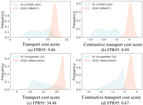
Ablation on virtual outliers We compare the OOD detection performance of POT with and without virtual outliers, which are generated to approximate the OOD region using linear representation extrapolation. Figure 3 displays the results, where we visualize the data distribution in the CIFAR100 and ImageNet-1k benchmarks. Using the virtual outliers leads to clearer separability between ID and OOD samples, whereas the transport cost score without virtual outliers exhibits larger overlap. The results show that the introduction of virtual outliers enhances the distinguishability between ID and OOD, resulting in more effective OOD detection.
Parameter analysis We ablate along individual parameters with ImageNet-1k as ID data, shown in Figure 6.4 in Appendix 6.4 , where the ViT-b16 is utilized as the backbone for analysis. In Figure 6.4 (a), we find that increasing the test batch size is beneficial for OOD detection. We hypothesize that this improvement is due to larger batch sizes providing a better empirical approximation of the true test data distribution, thereby enabling more accurate measurement of distributional discrepancies and improving detection performance. Although POT faces a performance degradation with the decrease of test batch size, its performance of lower batch sizes still hold superiority over the baseline methods. For instance, POT already achieves 93.18% average AUROC with the test batch size of 32, which outperforms the competitive rival NAC-UE (see Table 1). In Figure 6.4 (b), we can observe that as the regularization coefficient λ increases, AUROC undergoes an ascending interval followed by a decrease interval, ultimately leading to convergence. This convergence occurs because the entropy term becomes increasingly influential in the optimization of OT as λ increases, eventually leading to a uniform transport plan with maximum entropy, thereby stabilizing OOD detection performance. In Figure 6.4 (c), we find that POT works better with a moderate ω. This is intuitive as a lower ω may lead the generated virtual outliers close to ID samples, while a higher ω can generate virtual outliers far away both ID and OOD samples, leading the transport costs to virtual outliers indistinguishable.
| Benchmarks | OOD | Logits | Penultimate | ||
|---|---|---|---|---|---|
| FPR95↓ | AUROC↑ | FPR95↓ | AUROC↑ | ||
| CIFAR-100 | Far | 18.86 | 95.58 | 14.35 | 96.70 |
| Near | 45.68 | 85.38 | 44.28 | 86.51 | |
| ImageNet-1k | Far | 20.26 | 95.49 | 15.59 | 96.78 |
| Near | 67.97 | 80.45 | 60.15 | 83.95 | |
Penultimate layer vs. logit layer In this paper, we follow the convention in feature-based methods by using the representations from the penultimate layer of neural network, as it is believed to preserve more information than the output from the top layer, also referred to as logits. To investigate the impact of layer selection, we provide evaluation on POT using representations from the penultimate layer or logits, with the average results presented in Table 6. From the results, using the representations from the penultimate layer achieves better performance than using the logits.
5 Conclusion
In this paper, we tackle the problem of OOD detection from a new perspective of measuring distribution discrepancy and quantifying the individual contribution of each test input. To this end, we propose a novel method named POT, which utilizes the prototype-based OT to assess the discrepancy between test inputs and ID prototypes and use the obtaining transport costs for OOD detection. By generating virtual outliers to approximate the OOD region, we combine the transport costs to ID prototypes with the costs to virtual outliers, resulting in a more effective contrastive transport cost for identifying OOD inputs. Experimental results demonstrate that POT achieves better performance than 21 current methods. Moreover, we show that POT is pluggable with existing training methods for OOD detection and is applicable to the scenarios where the training data is unavailable, highlighting its generic nature and high practicality.
Acknowledgements
This work was supported in part by the National Natural Science Foundation of China under Grant 62472400, Grant 62072428, Grant 62271465, and in part by the Suzhou Basic Research Program under Grant SYG202338. Xike Xie is the corresponding author.
@inproceedings{ijcai2025p336,
  title     = {Prototype-based Optimal Transport for Out-of-Distribution Detection},
  author    = {Ke, Ao and Chen, Wenlong and Feng, Chuanwen and Cao, Yukun and Xie, Xike and Zhou, S. Kevin and Feng, Lei},
  booktitle = {Proceedings of the Thirty-Fourth International Joint Conference on
               Artificial Intelligence, {IJCAI-25}},
  publisher = {International Joint Conferences on Artificial Intelligence Organization},
  editor    = {James Kwok},
  pages     = {3018--3026},
  year      = {2025},
  month     = {8},
  note      = {Main Track},
  doi       = {10.24963/ijcai.2025/336},
  url       = {https://doi.org/10.24963/ijcai.2025/336},
}
TY - CPAPER TI - Prototype-based Optimal Transport for Out-of-Distribution Detection AU - Ke, Ao AU - Chen, Wenlong AU - Feng, Chuanwen AU - Cao, Yukun AU - Xie, Xike AU - Zhou, S. Kevin AU - Feng, Lei T2 - Proceedings of the Thirty-Fourth International Joint Conference on Artificial Intelligence, IJCAI-25 PB - International Joint Conferences on Artificial Intelligence Organization PY - 2025 SP - 3018 EP - 3026 DO - 10.24963/ijcai.2025/336 UR - https://doi.org/10.24963/ijcai.2025/336 ER -Copied
Machine-readable versions of this paper, for tools and AI agents:





