
Finding Possible Winners in Spatial Voting with Incomplete Information
Proceedings of the Thirty-Fourth International Joint Conference on Artificial Intelligence. Main Track. Pages 4048-4056.
https://doi.org/10.24963/ijcai.2025/451
Keywords
- Game Theory and Economic Paradigms: GTEP: Computational social choice
- Planning and Scheduling: PS: Scheduling
Abstract
We consider a spatial voting model where both candidates and voters are positioned in the d-dimensional Euclidean space, and each voter ranks candidates based on their proximity to the voter's ideal point. We focus on the scenario where the given information about the locations of the voters' ideal points is incomplete; for each dimension, only an interval of possible values is known. In this context, we investigate the computational complexity of determining the possible winners under positional scoring rules. Our results show that the possible winner problem in one dimension is solvable in polynomial time for all k-truncated voting rules with constant k. Moreover, for some scoring rules for which the possible winner problem is NP-complete, such as approval voting for any dimension or k-approval for two or more dimensions, we give an FPT algorithm parameterized by the number of candidates. Finally, we classify tractable and intractable settings of the em weighted possible winner problem in one dimension, and resolve the computational complexity of the weighted case for all two-valued positional scoring rules when d=1.
- [Alós-Ferrer and Granić, 2015] Carlos Alós-Ferrer and Georg Dura Granić. Political space representations with approval data. Electoral Studies, 39:56-71, January 2015.
- [Baptiste, 2000] Philippe Baptiste. Scheduling equal-length jobs on identical parallel machines. Discrete Applied Mathematics, 103(1-3):21-32, 2000.
- [Bartholdi et al., 1989] John J Bartholdi, Craig A Tovey, and Michael A Trick. The computational difficulty of manipu- lating an election. Social choice and welfare, 6:227-241, 1989.
- [Baumeister and Rothe, 2012] Dorothea Baumeister and Jörg Rothe. Taking the final step to a full dichotomy of the possible winner problem in pure scoring rules. Information Processing Letters, 112(5):186-190, 2012.
- [Baumeister et al., 2012a] Dorothea Baumeister, Piotr Fal- iszewski, Jérôme Lang, and Jörg Rothe. Campaigns for lazy voters: truncated ballots. In AAMAS, pages 577-584, 2012.
- [Baumeister et al., 2012b] Dorothea Baumeister, Magnus Roos, Jörg Rothe, Lena Schend, and Lirong Xia. The possible winner problem with uncertain weights. In ECAI 2012, pages 133-138. IOS Press, 2012.
- [Betzler and Dorn, 2010] Nadja Betzler and Britta Dorn. To- wards a dichotomy for the possible winner problem in elections based on scoring rules. Journal of Computer and System Sciences, 76(8):812-836, 2010.
- [Black, 1948] Duncan Black. On the rationale of group decision-making. Journal of political economy, 56(1):23- 34, 1948.
- [Bogomolnaia and Laslier, 2007] Anna Bogomolnaia and Jean-Franc ¸ois Laslier. Euclidean preferences. Journal of Mathematical Economics, 43(2):87-98, 2007.
- [Brandt et al., 2015] Felix Brandt, Markus Brill, Edith Hemaspaandra, and Lane A Hemaspaandra. Bypassing combinatorial protections: Polynomial-time algorithms for single-peaked electorates. Journal of Artificial Intel- ligence Research, 53:439-496, 2015.
- [Brandt et al., 2016] Felix Brandt, Vincent Conitzer, Ulle Endriss, Jérôme Lang, and Ariel D Procaccia. Handbook of computational social choice. Cambridge University Press, 2016.
- [Conitzer and Sandholm, 2002] Vincent Conitzer and Tuo- mas Sandholm. Complexity of manipulating elections with few candidates. In AAAI/IAAI, pages 314-319, 2002.
- [Conitzer et al., 2007] Vincent Conitzer, Tuomas Sandholm, and Jérôme Lang. When are elections with few candi- dates hard to manipulate? Journal of the ACM (JACM), 54(3):14-es, 2007.
- [Cygan et al., 2015] Marek Cygan, Fedor V Fomin, Łukasz Kowalik, Daniel Lokshtanov, Dániel Marx, Marcin Pilipczuk, Michał Pilipczuk, and Saket Saurabh. Parame- terized algorithms, volume 5. 2015.
- [Dogan and Giritligil, 2014] Onur Dogan and Ayc ¸a Ebru Giritligil. Implementing the borda outcome via truncated scoring rules: a computational study. Public Choice, 159:83-98, 2014.
- [Downey et al., 2013] Rodney G Downey, Michael R Fel- lows, et al. Fundamentals of parameterized complexity, volume 4. 2013.
- [Elkind et al., 2022] Edith Elkind, Martin Lackner, and Do- minik Peters. Preference restrictions in computational so- cial choice: A survey. arXiv preprint arXiv:2205.09092, 2022.
- [Faliszewski et al., 2009] Piotr Faliszewski, Edith Hemas- paandra, Lane A Hemaspaandra, and Jörg Rothe. The shield that never was: Societies with single-peaked prefer- ences are more open to manipulation and control. In Pro- ceedings of the 12th Conference on Theoretical Aspects of Rationality and Knowledge, pages 118-127, 2009.
- [Grigor'ev and Vorobjov Jr, 1988] D Yu Grigor'ev and Nico- lai N Vorobjov Jr. Solving systems of polynomial inequal- ities in subexponential time. Journal of symbolic compu- tation, 5(1-2):37-64, 1988.
- [Imber et al., 2024] Aviram Imber, Jonas Israel, Markus Brill, Hadas Shachnai, and Benny Kimelfeld. Spatial vot- ing with incomplete voter information. In Proceedings of the AAAI Conference on Artificial Intelligence, volume 38, pages 9790-9797, 2024.
- [Kimelfeld et al., 2019] Benny Kimelfeld, Phokion G Ko- laitis, and Muhammad Tibi. Query evaluation in election databases. In Proceedings of the 38th ACM SIGMOD- SIGACT-SIGAI Symposium on Principles of Database Sys- tems, pages 32-46, 2019.
- [Konczak and Lang, 2005] Kathrin Konczak and Jérôme Lang. Voting procedures with incomplete preferences. In Proc. IJCAI-05 Multidisciplinary Workshop on Advances in Preference Handling, volume 20, 2005.
- [Lenstra Jr, 1983] Hendrik W Lenstra Jr. Integer program- ming with a fixed number of variables. Mathematics of operations research, 8(4):538-548, 1983.
- [Moulin, 1984] Hervé Moulin. Generalized condorcet- winners for single peaked and single-plateau preferences. Social Choice and Welfare, 1(2):127-147, 1984.
- [Niedermeier, 2002] Rolf Niedermeier. Invitation to fixed- parameter algorithms. Habilitationschrift, University of Tübingen, 19, 2002.
- [Pini et al., 2011] Maria Silvia Pini, Francesca Rossi, Kris- ten Brent Venable, and Toby Walsh. Incompleteness and incomparability in preference aggregation: Complexity re- sults. Artificial Intelligence, 175(7-8):1272-1289, 2011.
- [Reis and Rothvoss, 2023] Victor Reis and Thomas Rothvoss. The subspace flatness conjecture and faster integer programming. In 2023 IEEE 64th Annual Sympo- sium on Foundations of Computer Science (FOCS 2023), pages 974-988, 2023.
- [Shachnai et al., 2025] Hadas Shachnai, Rotem Shavitt, and Andreas Wise. Finding possible winners in spatial voting with incomplete information. arXiv preprint arXiv:2505.12451, 2025.
- [Stockemer et al., 2018] Daniel Stockemer, André Blais, Filip Kostelka, and Chris Chhim. Voting in the eurovision song contest. Politics, 38(4):428-442, 2018.
- [Terzopoulou and Endriss, 2021] Zoi Terzopoulou and Ulle Endriss. The borda class: An axiomatic study of the borda rule on top-truncated preferences. Journal of Mathemati- cal Economics, 92:31-40, 2021.
- [Walsh, 2007] Toby Walsh. Uncertainty in preference elic- itation and aggregation. In AAAI, volume 7, pages 3-8, 2007.
- [Yang, 2017] Yongjie Yang. On the complexity of borda con- trol in single-peaked elections. In Proceedings of the 16th Conference on Autonomous Agents and MultiAgent Sys- tems, pages 1178-1186, 2017.
References were extracted automatically from the PDF and may contain errors.
Full text extracted automatically from the PDF; figures, tables and equations may differ. The PDF is the version of record.
1 Introduction
The spatial model of voting associates voters and candidates with points in the d-dimensional Euclidean space, i.e., in Rd . Each dimension corresponds to an issue on which the voters and the candidates have an opinion; this opinion is defined by the coordinate of the voter or candidate in this dimension. Voters prefer candidates closer to their respective point (measured as the Euclidean distance in Rd ) over those who are further away. Hence, for each voter this induces an order of the candidates. In the social choice literature, preferences with this structure are often referred to as (d-)Euclidean preferences [Bogomolnaia and Laslier, 2007; Elkind et al., 2022]. The most common example of a spatial model is a political spectrum, such as the traditional left-right axis where d = 1, but issue spaces can be of higher dimension (see, e.g., [Al´os-Ferrer and Grani´c, 2015]).
∗Corresponding author
We consider a common scenario where the point in Rd of each candidate is known precisely, e.g., from the election campaign, but for the voters' preferences only partial information is available. For each voter and each of the d dimensions, we assume that we are given an interval which contains the opinion of the voter corresponding to this dimension. This model captures the real-world uncertainty present in political elections, where it is difficult to determine precisely which party a voter supports. However, we can often estimate a general range for their political views-for example, whether they lean left or right. From this partial information we can identify a set of possible preference orders for the voter.
We study voting systems in which there is a global scoring vector ⃗sm = (sm(1), sm(2), ..., sm(m)), depending on the number of candidates, with sm(1) ≥ sm(2) ≥ ... ≥ sm(m) such that each voter assigns a score of sm(1) to her favorite candidate, a score of sm(2) to her second favorite candidate, and so on. Also, we study approval voting where each voter vj casts a vote to each candidate whose opinion is within a given approval radius ρj of the point in Rd corresponding to vj. In both settings, we say that a candidate can win the election if no other candidate receives a higher total score.
Since the precise opinion of each voter is not known, it is unclear which candidate will win the election. Two key questions arising in this setting are whether a specific candidate can be a possible winner (who wins in at least one scenario by the opinions of the voters) or a necessary winner (one who wins in every possible scenario). These questions, introduced in the seminal work of [Konczak and Lang, 2005], have garnered significant attention in various settings involving incomplete information about voters' preferences (see Section 1.1).
The necessary winner problem (NW) is well understood in this model, thanks to a thorough study in [Imber et al., 2024]. However, the complexity of PW⟨d⟩, i.e., the possible winner problem with incomplete voters' information in d dimensions, is known only for certain classes of positional scoring rules. Specifically, as shown in [Imber et al., 2024], PW⟨1⟩ is solvable in polynomial time for all two-valued rules, i.e., rules in which the vector ⃗s contains only two different values, and for two specific families of rules with more than two values. On the other hand, PW⟨d⟩ is NP-complete for any number of dimensions d ≥ 2, already for the (relatively simple) scoring vector ⃗s = (1, 1, 1, 0, ..., 0) [Imber et al., 2024].
| Problem | k-approval | Multi-valued positional scoring rules | Approval voting |
|---|---|---|---|
| PW⟨1⟩ | in P [Imber et al., 2024] | in P for any k-truncated scoring rule for a constant k [Theorem 1] | NP-c [Imber et al., 2024] FPT in m [Theorem 3] |
| PW⟨d⟩ | NP-c for k ≥ 3, d ≥ 2 [Imber et al., 2024], FPT in m [Theorem 2] | FPT in m [Theorem 2] | NP-c [Imber et al., 2024] FPT in m [Theorem 3] |
| WPW⟨1⟩ | in P if k(m) ≥ m2 ∀m ∈ N, otherwise NP-c [Theorem 4] | NP-c for Borda with m ≥ 4 [Theorem 5] | NP-c [Imber et al., 2024] |
These previous results leave several intriguing questions open: (1) Is PW⟨1⟩ still tractable for other positional scoring rules with more than two values, e.g., for ⃗s = (2, 1, 0, ..., 0)? (2) For voting rules under which PW⟨d⟩ is NP-complete, can we devise parameterized algorithms? (3) What happens if each voter is associated with a weight, e.g., representing a group of voters sharing the same (unknown) common opinion, or members with varying levels of influence in a board of directors? Is the weighted possible winner problemWPW⟨d⟩ harder than PW⟨d⟩? We answer all three questions positively, see Table 1 for an overview.
First, we present a polynomial-time algorithm for PW⟨1⟩ for any scoring rule with a constant number of nonzero entries. Such scoring rules are very common in real-life voting systems: the Eurovision Song Contest [Stockemer et al., 2018]) uses the scoring vector (12, 10, 8, 7, 6, 5, 4, 3, 2, 1, 0..., 0) and the NBA MVP contest uses (10, 7, 5, 3, 1, 0, . . . , 0). Also, this class contains the ktruncated Borda rule (k, k - 1, ..., 1, 0, . . . , 0) which is used in the NCAA Football Division 1A Coaches' poll for k = 25.
Such scoring rules are popular because ranking all candidates becomes impractical when their number is large. Moreover, voters often lack strong preferences beyond their top choices, making the order among lower-ranked candidates irrelevant. Also, keeping the number of positive entries fixed ensures stability in the voting system in repeated contests as described above, where the number of candidates may vary, and a voting rule that depends on this number complicates the process and hinders comparisons across events.
Our algorithm reduces PW to the problem of shapes scheduling. To the best of our knowledge, this scheduling setting has not been studied before and it might be of independent interest. We solve the resulting instances of this problem, building on a technique of [Baptiste, 2000].
In real elections, the number of candidates m (with realistic chances of winning) is typically rather small. This motivates us to choose m as a fixed parameter. We show that for any dimension d (not necessarily constant or bounded by a fixed parameter) the problem PW⟨d⟩ becomes fixed-parameter tractable (FPT) for any positional scoring rule and also for approval voting (we use standard terminology in parameterized complexity [Downey et al., 2013; Cygan et al., 2015; Niedermeier, 2002]). Thus, we can solve the problem in time f(m) · nO(1) , for some computable function f.
Finally, we prove that WPW⟨d⟩ is NP-complete already when d = 1 and m = 4 under the Borda scoring rule.
In contrast, our result above shows that the corresponding unweighted case admits a polynomial time algorithm. In addition, we resolve the computational complexity of the weighted possible winner problem for all two-valued positional scoring rules when d = 1, by distinguishing between scoring rules which remain tractable, and others under which WPW⟨1⟩ becomes NP-complete (for short, NP-c).
1.1 RelatedWork
In voting theory, partial information has been explored under various voting models. [Konczak and Lang, 2005] introduced the partial order model, where each voter's preferences are specified as a partial order rather than a complete ranking. They also formulated the two fundamental problems of necessary winner and possible winner, which analyze the conditions under which candidates can be guaranteed or potentially elected given the incomplete preferences. [Betzler and Dorn, 2010] established the computational complexity of PW within the partial order model for all scoring rules except for (2, 1, . . . , 1, 0). Specifically, they show that PW is solvable in polynomial time under the plurality and veto voting rules, while for other scoring rules it is NP-complete. [Baumeister and Rothe, 2012] extended the hardness results to the (2, 1, . . . , 1, 0) voting rule.
Truncated voting rules (or truncated ballots) are used to simplify voting procedures. [Baumeister et al., 2012a] study the complexity of determining a PW given truncated ballots. [Yang, 2017] and [Terzopoulou and Endriss, 2021] studied elections under different variants of truncated Borda scoring rules. [Do˘gan and Giritligil, 2014] investigated the likelihood of choosing the Borda outcome using a truncated scoring rule.
Weighted voting models, where voter influence is weighted, have been explored extensively [Bartholdi et al., 1989; Brandt et al., 2016; Conitzer and Sandholm, 2002; Conitzer et al., 2007]. [Pini et al., 2011] studied NW and PW with weighted voters in the partial orders model, and showed NP-hardness results for Borda, Copland, Simpson, and STV rules. [Walsh, 2007] extended these results to cases where the number of candidates is bounded. [Baumeister et al., 2012b] analyzed weighted PW where voter preferences are known but weights are unknown.
Spatial voting generalizes single-peaked preferences by embedding voters and candidates in a multidimensional space, where preferences are single-peaked along certain dimensions. Single-peaked preferences, first studied by [Black, 1948], have been widely analyzed for their simplifying effects on voting problems such as manipulation and winner determination under many voting rules [Brandt et al., 2015; Moulin, 1984]. [Faliszewski et al., 2009] show that NPhardness of manipulation and control vanishes under singlepeak preferences. On the other hand, the hardness result remains for weighted elections. In Section 5 we adjust some of these results for WPW⟨1⟩.
Additional related work is discussed in the full version of the paper [Shachnai et al., 2025].
2 Preliminaries
Spatial Voting. Let V = {v1, . . . , vn} denote the set of voters and C = {c1, . . . , cm} the set of candidates, where m ≥ 2 to avoid trivial cases. Every candidate has a position in the d-dimensional space representing their opinions on d issues. 1 Each voter vi has a ranking Ri over all candidates. The collection of all rankings for all the voters forms a ranking profile, denoted by R = (R1, . . . , Rn).
A spatial voting profile T = (T1, ..., Tn) consists of n points, where Tj = ⟨Tj,1, . . . , Tj,d⟩ ∈ Rd represents voter vj's opinion on d issues. Given a spatial voting profile T, RT = (RT1 , ...,RTn ) is the derived ranking profile, where each voter vj ranks candidates in C according to their distance from vj's opinion, Tj. The closest candidate is ranked first, and the farthest is ranked in position m in vj's preferences. Tie breaking rule is arbitrary but fixed for all voters.
Voting Rules. A voting rule is a function that maps a ranking profile to a nonempty set of winners. This paper focuses mainly on positional scoring rules, where candidates earn points based on their rank positions. A positional scoring rule r is defined as a sequence {⃗sm}m≥2 of m-dimensional score vectors ⃗sm = (sm(1), . . . , sm(m)). For each m ∈ N the vector ⃗sm consists of m natural numbers that satisfy sm(1) ≥ · · · ≥ sm(m), and s1(m) > sm(m).
For a ranking profile R = (R1, ...,Rn) and a positional scoring rule r with a score vector ⃗sm, the score assigned to candidate c by voter vj is s(Rj , c) = sm(i), where c is ranked in the i-th position in Rj . The total score of candidate c is denoted by s(R, c) = ∑nj=1 s(Rj , c). Examples for positional scoring rules include plurality (1, 0, ..., 0), veto (1, ..., 1, 0), k-approval (1, . . . , 1, 0, . . . , 0) where the number of '1' entries is k, and the Borda rule, where the scoring vector is (m - 1, m - 2, ..., 0).
A two-valued positional scoring rule consists of two values which are w.l.o.g. '1' and '0'. Such rules can be described as k(m)-approval, where for m candidates, the m-dimensional score vector ⃗sm consists of k(m) '1' entries. Note that throughout the paper, when using the term k-approval, we refer to a fixed value of k (which does not depend on m).
One focus of this paper is a subclass of positional scoring rules called truncated scoring rules [Do˘gan and Giritligil, 2014]. In a k-truncated scoring rule, each score vector ⃗sm has strictly positive values only in its first k entries. Thus, a it allows voters to allocate score to exactly k candidates.
Partial Spatial Voting. [Imber et al., 2024] introduced the partial spatial voting model, where voters' preferences are incompletely specified. This model is represented by a partial spatial profile P = (P1, . . . , Pn), where each voter vj is described as a vector of intervals Pj = ⟨[ℓj,1, uj,1], . . . , [ℓj,d, uj,d]⟩, and [ℓj,i, uj,i] represents the lower and upper bounds of vj's ideal point in each issue. The precise positions of the candidates are assumed to be known. A spatial voting profile T = (T1, . . . , Tn) is a spatial completion of P if, for every voter vj, Tj,i ∈ [ℓj,i, uj,i]. The ranking profile RT is then derived from this completion.
1 For the case of d = 1, we assume c1 < c2 < · · · < cm.
Definition 1. Given a partial profile P and a candidate c∗ ∈ C, the possible winner problem under a voting rule r asks whether there exists a profile completion T of P such that c∗ is a winner w.r.t. r, i.e., s(RT, c∗ ) ≥ s(RT, c) ∀ c ∈ C.
Spatial Approval Voting. In approval voting, voters partition candidates into "approved" and "unapproved" groups, selecting the candidate with the highest approval count. Unlike k-approval, the number of approvals per voter varies. In spatial settings, each voter vj has an approval radius ρj ∈ R and approves candidates within a distance ρj . Given a spatial completion T, the approval set for voter vj is ATj = {c ∈ C : ∥Tj - c∥2 ≤ ρj}. Approval regions correspond to intersections of d-dimensional spheres and the voter's position rectangle.
3 PW⟨1⟩ with k-Truncated Voting Rules
In this section we establish that PW⟨1⟩ with any k-truncated voting rule can be solved in polynomial time when k is constant. To do so, we introduce a new multi-machine scheduling problem, termed shapes scheduling, where processing a job requires varying machine resources over time. We then provide a polynomial-time reduction from PW⟨1⟩ to the shapes scheduling problem. In the reduction, every voter becomes a job, and the resources used to process it reflect the score the voter hands to candidates. Finally, we present a dynamic programming algorithm to efficiently solve shapes scheduling instances.
3.1 The Shapes Scheduling Problem
In shapes scheduling each job may use multiple machines, in a quantity that changes over the processing time. Each scheduling option is referred to as a shape, which specifies the number of machines required at any time throughout processing. Assume that time is slotted. We first present the notion of a shape. Let [r] denote the set {1, . . . , r}.
Definition 2. Let p ∈ N. A shape f is a vector (M f 0 , ...,M f p-1 ) such that M f i ∈ N0 for each i ∈ {0} ∪ [p - 1]. We denote by p the processing time of f .
The intuition is that if job j is scheduled at time t ∈ N with a shape f and a processing time p then for each i ∈ {0} ∪ [p - 1], during the interval [t + i, t + i + 1) job j occupies M f i machines. For instance, consider the shape f = (2, 1) with p = 2. Figure 1 shows two ways to schedule the job at time t using f, both satisfying the requirement of two machines during [t, t+1) and one machine during [t+1, t+2). Note that the machine indices are irrelevant, and there is no requirement to use the same machine across consecutive time slots. Additionally, preemption is not allowed.
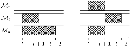
In the shapes scheduling problem we are given a set of M identical machines for some M ∈ N, and a set of jobs J. Each job j ∈ J is associated with (i) a processing time pj ∈ N, (ii) a release time rj ∈ N0, (iii) a deadline dj ∈ N with rj+pj ≤ dj, and (iv) a set of shapes F (j) t , each with processing time pj , for any time t ∈ N0 such that rj ≤ t ≤ dj - pj .
The goal is to select for each job j ∈ J a starting time Sj ∈ N0 satisfying rj ≤ Sj ≤ dj - pj and a shape f (j) ∈ F (j) t . Given these starting times and shapes, for each time t ∈ N we denote the number of busy machines during [t, t+1) by M(t). Formally, we define M(t) := ∑j∈J:Sj≤t<Sj+pj M f (j) t-Sj . We require for each t ∈ N0 that M(t) ≤ M, i.e., at most M machines are used during the interval [t, t + 1).
3.2 Reduction fromPW⟨1⟩ to Shapes Scheduling
We show how we can reduce PW⟨1⟩ to the shapes scheduling problem. Given an instance of PW⟨1⟩, the release times and deadlines of our jobs will be in the interval [1,m+ 1]; intuitively, for each i ∈ [m], the interval [i, i + 1) corresponds to candidate ci. For each voter vj ∈ V we define a job j ∈ J as follows. We set pj = k. Let iL be the smallest index such that candidate ciL receives a positive score from vj if Tj = ℓj . We set rj = iL. Similarly, let iR be the largest index such that candidate ciR receives a positive score from vj if Tj = uj. We set dj = iR + 1.
Lemma 1. For each possible position Tj ∈ [ℓj, uj] for voter vj , only candidates in {ciL , ..., ciR } receive a score from vj .
Next, we define the set of allowed shapes for j. Consider a value t ∈ [m] with rj ≤ t ≤ dj -k. Let Tj,t denote the set of possible positions Tj for vj such that exactly the candidates ct, ..., ct+k-1 receive a score, meaning these candidates are the top k candidates in RTj . For each Tj ∈ Tj,t and each i ∈ {0}∪[k-1], s(RTj , ct+i) is the score that candidate ct+i receives from voter vj if it is positioned at Tj. This yields a shape (s(RTj , ct), ..., s(RTj , ct+k-1)).
Figure 2 illustrates two possible positions of voter vj, denoted Tj and T ′ j . Let the scoring rule be 2-truncated Borda: s = (2, 1, 0 . . . , 0). At Tj, the ranking of vj is RTj = (c1, c2, c3), where the top two candidates are c1 and c2, implying Tj ∈ Tj,1. As s(RTj , c1) = 2 and s(RTj , c2) = 1, the resulting shape is f = (2, 1). At T ′ j , the ranking is RT ′ j = (c3, c2, c1), making c2 the lowest-indexed candidate in the top two. Therefore, T ′ j ∈ Tj,2, resulting in the shape f ′ = (1, 2).
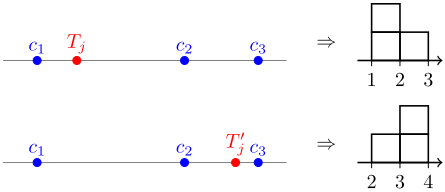
We define F (j) t to be the set of all these shapes, i.e., F (j) t := {(s(RTj , ct), ..., s(RTj , ct+k-1)) : Tj ∈ Tj,t}. We can compute the set F (j) t by showing that there is a subset of positions Tj in Tj,t that suffice for defining all shapes in F (j) t , and that we can construct this subset efficiently.
Lemma 2. For each voter vj and each t ∈ [m] with rj ≤ t ≤ dj - k we can compute the set F (j) t in time O(knm2 ).
Proof. For any pair of candidates ci < ch, the middle point mi,h = ch-ci 2 separates the space into two regions: every voter vj whose position is Tj ≤ mi,h prefers candidate ci over ch, and every voter vj whose position is Tj > mi,h prefers ch over ci. In this case, the tie breaking is in favor of the lower indexed candidate, though it can be adjusted to every fixed tie breaking rule. By finding the middle point for each pair of candidates, we separate the space into (m2 ) + 1 segments, where the ranking of candidates for all voters positioned in a given segment are the same.
For each segment E, denote by RE the ranking profile for voters positioned in segment E, i.e., RE = (cℓ1 , cℓ2 , . . . , cℓm ), where cℓ1 is the candidate who receives the highest number of votes, cℓ2 the second to highest, and so on. Let zE be the smallest index of a candidate who is in the top k candidates in RE. Note that zE is a non-decreasing series by the segment going left to right. We define a shape f(E) = (M f(E) 0 , . . . ,M f(E) k-1 ) for each segment as follows. For each i ∈ {0} ∪ [k - 1], the ith entry in the shape vector, M f (E) i , is the score candidate czE+i receives by the ranking profile of segment E, i.e. M f(E) i = s(RE, czE+i). For each voter vj and each t ∈ [m] with rj ≤ t ≤ dj - k, we can compute the set F (j) t . First, we define for every t ∈ [m], Ft = {f(E)| ∀E : zE = t}. Let vj ∈ V with Pj = [ℓj, uj].
- For every t such that rj < t < dj - k: F (j) t = Ft.
- F (j) rj = {f(E)| ∀E : zE = rj ∧ (E ∩ [ℓj, uj] ̸= ∅)}.
- F (j) dj = {f(E)| ∀E : zE = dj -k∧(E∩[ℓj, uj] ̸= ∅)}.
It holds that F (j) t ⊆ Ft for every job j and time t.
We constructed the set F (j) t for each job j and each value t ∈ [m] with rj ≤ t ≤ dj - k. Now we show that for each job j, the possible starting times and their associated shapes represent a possible assignment of scores by voter vj to the candidates, depending on the position Tj of vj .
Lemma 3. For each job j ∈ J there is a starting time Sj and a shape f (j) ∈ F (j) Sj if and only if there is a position Tj ∈ [ℓj, uj] for voter vj such that for every i ∈ {0}∪[k-1], vj gives a score of M f (j) i to candidate cSj+i.
Proof. We start with the first direction. Let j ∈ J be a job scheduled at Sj in shape f (j) ∈ F (j) Sj . We define a position Tj ∈ [ℓj, uj] such that vj gives a score of M f (j) i to candidate cSj+i for all i ∈ {0} ∪ [k - 1]. As f (j) ∈ F (j) Sj , by the construction of F (j) Sj there exists a segment E such that E ∩ Pj ̸= ∅, zE = Sj and f(E) = f (j) . We define the position of vj to be a point Tj ∈ E ∩ Pj, which is valid because Tj ∈ Pj. Recall that the shape f(E) is defined such that for each i ∈ {0}∪[k-1], M f(E) i is the number of votes given to czE+i by a voter positioned in E, as M f(E) i = s(RE, czE+i); therefore, for every such i, the number of votes given by vj to cSj+i is the number of votes given to czE+i, i.e., vj gives M f (E) i votes to candidate cSj+i.
We continue with the second direction. Let Tj ∈ [ℓj , uj ] be a position for voter vj such that vj gives s(RTj , cSj+i) votes to candidate cSj+i for every i ∈ {0} ∪ [k - 1]. Let E be the segment such that Tj ∈ E. We define the starting time of j, to be Sj = zE and the scheduling shape of j to be f(E), and show that rj ≤ Sj ≤ dj - k, M f(E) i = s(RTj , cSj+i) for every i ∈ {0} ∪ [k - 1] and f(E) ∈ F (j) Sj .
By Lemma 1, if candidate cSj receives a score from vj then iL ≤ Sj, where ciL is the smallest candidate to receive a positive number, and rj = iL ≤ Sj. Also, Sj + k - 1 ≤ iR, where cIR is the largest candidate to receive a positive number, and dj = iR + 1 ≥ Sj + k. By definition of f(E), M f (E) i = s(RTj , cSj+i-1). By the construction of the shape sets, for every segment E ∩ [ℓj, uj] with a scheduling time rj ≤ Sj ≤ dj, it holds that f(E) ∈ F (j) Sj .
The next step is to combine Lemma 1 and Lemma 3 to establish the correctness of the reduction.
Lemma 4. Let i∗ ∈ [m] be the index of candidate c∗ . Then, candidate c∗ is a possible winner if and only if there is a number M ∗ ∈ {∑i∈I sm(i)|∀i ∈ I, i ∈ [k], |I| ≤ n} such that for the set of jobs J there is a feasible schedule with M ∗ machines such that all machines are busy during [i∗ , i∗ + 1).
The intuition behind this is that every use of machine at a time slot [t, t + 1) corresponds to a score given to candidate t (Lemma 3); therefore, if all machines are busy at c∗ , the schedule corresponds to a profile completion in which candidate c∗ receives M ∗ votes, and no other candidate receives more, since there are only M ∗ machines.
3.3 An Algorithm for Shapes Scheduling
Our algorithm decides if there is a solution to the shapes scheduling instance which satisfies Lemma 4. The algorithm exploits certain properties of the sets of possible shapes F (j) t . To this end, we define the notion of P-structured jobs.
Definition 3. Let J be a set of jobs in an instance of shapes scheduling, and let P ∈ N. The set J is P-structured if
- pj = P for each job j ∈ J,
- for each t ∈ N0 there is a global set Ft such that if t ̸= rj, dj, then F (j) t = Ft,
- There exists an order of the jobs such that, for every two jobs j, j ′ ∈ J, if j ≺ j ′ then either dj < dj ′ or dj = dj ′ and F (j) dj ⊆ F (j ′ ) dj′ .
Due to our construction of the instance J, we can show that for P = k, the jobs are P-structured.
Lemma 5. The job set J generated by the reduction is Pstructured for P = k.
We now present an algorithm for any P -structured instance of scheduling with shapes. Given a set of P-structured jobs J, a candidate c∗ ∈ C, and a number of machines M ∗ , our algorithm decides if there exists a schedule for J with M ∗ machines such that all machines are busy at time c∗ . Then, we run the algorithm for every possible value of M ∗ . This can be done in polynomial time since M ∗ must be a combination of n votes, each of value sm(1), sm(2), . . . , sm(k) or 0. The heart of our algorithm is formalized as Lemma 6, which generalizes a result of [Baptiste, 2000]. Intuitively, our lemma states that if there is a feasible schedule with M ∗ machines, then there is also a feasible schedule in which a job j ′ with the latest deadline among all jobs in J starts at a time Sj ′ such that the remaining jobs are split nicely into two parts:
- a set JL containing all jobs j ∈ J \ {j ′ } with rj < Sj ′ and for each job j ∈ JL we have Sj ≤ Sj ′ , and
- a set JR containing all jobs j ∈ J \ {j ′ } with rj ≥ Sj ′ ; thus, for each job j ∈ JR we have Sj ≥ Sj ′ .
This allows to partition our problem into two independent subproblems, one for JL and one for JR, on which we recurse. We define a total order ≺ for the jobs in J such that for any two jobs j, j ′ ∈ J we have j ≺ j ′ if dj < dj ′ , or if dj = dj ′ and F (j) dj ⊆ F (j ′ ) dj′ . Such order exists by Lemma 5. Using this order, we define the notation Uj ′ (t, t′ ) for subsets of jobs that we use below.
Definition 4. For any j ′ ∈ J and t, t′ ∈ N0, let Uj ′(t, t′ ) = {j | (j ⪯ j ′ ) ∧ (t ≤ rj < t′ )}.
Note that if j ′ is the last job in the total order ≺ among all jobs in J then J = Uj ′(0, dj ′). We now formalize the partition of our problem into two independent subproblems.
Lemma 6. Consider an instance of shapes scheduling with a set of P-structured jobs Uj ′(t, t′ ) where j ′ ∈ Uj ′(t, t′ ), and let j ′′ ∈ Uj ′(t, t′ ) such that j ≺ j ′′ for all j ∈ Uj ′(t, t′ ), j ̸= j ′ . Assume there is a schedule with a corresponding value M(t) for each t ∈ N0. Then there exists also a schedule with job start times (Sj)j∈J , the same value M(t) for each t ∈ N, and a partition of Uj ′ (t, t′ ) into three sets {j ′ }, JL,and JR such that
- JL = {j ∈ Uj ′′(t, t′ ) : rj < Sj ′} = Uj ′′(t, Sj ′) and Sj ≤ Sj ′ for each job j ∈ JL, and
- JR = {j ∈ Uj ′′(t, t′ ) : rj ≥ Sj ′} = Uj ′′(Sj ′ , t′ ) and Sj ≥ Sj ′ for each job j ∈ JR.
Assume that in our given instance, job j ′ is last in the total order ≺ of J. Algorithmically, we guess Sj ′ in polynomial time (as there are only a polynomial number of options). Once we guess Sj ′ correctly, we directly obtain JL and JR. Note that during each time interval [t, t + 1) with t ∈ N0 and t < Sj ′ we can process only jobs from JL. On the other hand, during each time interval [t′ , t′ + 1) with t′ ∈ N0 and t′ ≥ Sj ′ + P we can process only jobs from JR. During [Sj ′ , Sj ′ +P ) we may process jobs from JL but possibly also jobs from JR. Therefore, we also guess how to split the available machines between these two job sets during these time intervals. Formally, we define ML(t) to be the number of machines allocated to JL at time t, and similarly MR(t) to be the number of machines allocated to JR at time t. It must hold that ML(t) + MR(t) + M f t ≤ M ∗ for any t; therefore, we guess ML(Sj ′ ), . . . ,ML(Sj ′ + P - 1), and assign the remaining machines to JR during [Sj ′ , Sj ′ + P), i.e., we define MR(Sj ′ + i) := M ∗ -ML(Sj ′ + i) -M f i for any i ∈ {0} ∪ [P - 1]. Each value of ML(t) is a combination of n votes, therefore belongs to the set {∑i∈I sm(i)|∀i ∈ I, i ∈ [k], |I| ≤ n}, meaning it has (n+k n ) = O(nk ) options.
This yields independent subproblems for JL and JR on which we recurse. To ensure that running time is polynomial in the input size, we embed this recursion into a dynamic program with a polynomial number of DP-cells. Each subproblem is associated with an interval [t, t′ ) and a job j ′ , and we want to schedule the jobs j ≺ j ′ that are released during [t, t′ ), i.e. Uj ′ (t, t′ ). During [t, t + P) ∪ [t′ , t′ + P) we may not have all M ∗ machines available, as during these intervals our subproblem may interact with other (previously defined) subproblems. The DP-cell specifies how many machines are available during these intervals.
Formally, each DP-cell is defined by a tuple (j ′ , t, t′ ,Mt, . . . ,Mt+P-1,Mt′ , . . . ,Mt′+P-1) such that
- the values t, t′ ∈ N0 define an interval [t, t′ ),
- j ′ ∈ J is the last job according to ≺ of the input jobs of the subproblem,
- the values Mt, . . . ,Mt+P-1, ∈ {M ∗ - ∑i∈I sm(i)|∀i ∈ I, i ∈ [k], |I| ≤ n} denote the number of available machines during [t, t + 1), . . . , [t + P - 1, t + P ).
- the values Mt′ , . . . ,Mt′+P-1 ∈ {∑i∈I sm(i)|∀i ∈ I, i ∈ [k], |I| ≤ n} denote the number of available machines during [t′ , t′ + 1), . . . , [t′ + P - 1, t′ + P); note that the time points t, . . . , t + P - 1, t′ , . . . , t′ + P - 1 may not be pairwise distinct.
Recall that M(t) denotes the number of busy machines during [t, t + 1). The goal of this subproblem is to compute a schedule for the jobs Uj ′(t, t′ ) such that M(t + i) ≤ Mt+i,M(t′ + i) ≤ Mt′+i for any i ∈ {0} ∪ [P - 1], and M(t′′ ) ≤ M ∗ for each t′′ ∈ N0 with t + P ≤ t′′ < t′ . For i∗ being the index of candidate c∗ , if i∗ ∈ {t + P, ..., t′ - 1} we require that M(i∗ ) = M ∗ ; otherwise, we require that M(i∗ ) = Mi∗. Observe that the cell (n, 1,m - P +
1,M ∗ ,M ∗ ,M ∗ ,M ∗ ) corresponds to the main problem we want to solve, where n is the last job in the order ≺ of J. Based on these DP-cells, we can construct a dynamic program which decides whether there exists a feasible schedule for the given set of jobs.
Lemma 7. Assume we are given an instance of the shape scheduling problem with a set of P-structured jobs, M ∗ machines and a candidate c∗ ∈ C with index i∗ ∈ [m]. There is an algorithm with a running time of O(n1+3P 2 · m3 ) which decides whether the instance admits a feasible schedule in which all machines are busy during [i∗ , i∗ + 1).
Now, Lemmas 4 and 7 imply the next result.
Theorem 1. We can solve the possible winner problem for any k-truncated voting rule in time O(n1+k+3k2 · m3 ).
Our algorithm requires the input jobs to be P-structured, allowing us to solve the problem in polynomial time for constant P. In the full version of this paper [Shachnai et al., 2025], we complement this by showing that scheduling with shapes is strongly NP-hard if we lift these requirements.
4 Parameterized Algorithm for PW⟨d⟩
We present a parameterized algorithm for the PW problem in the d-dimensional euclidean space for any d ≥ 1. Our fixed parameter is the number of candidates m.
First, we describe our algorithm for positional scoring rules. Recall that we are given a score vector ⃗sm = (sm(1), ..., sm(m)), and each voter gives a certain number of votes to each candidate, according to ⃗sm. We say that a vector z = (z1, ..., zm) ∈ Nm0 is a voting vector if z describes the number of votes that a voter may give to each of the candidates, i.e., formally, if there is a permutation σ : [m] → [m] such that zi = sm(σ(i)) for each i ∈ [m]. We denote by Z the set of all voting vectors. Recall that each voter vj is described as a vector of intervals Pj = ⟨[ℓj,1, uj,1], . . . , [ℓj,d, uj,d]⟩. In particular, each voter vj may vote only for a subset of the voting vectors Z. We characterize the voters by the subsets of Z to which they may vote for. Therefore, for each subset of Z we introduce a corresponding type; formally, we define the set of types T to be all subsets of Z. We say that a voter vj is of some type τ ∈ T if vj may vote for exactly the subsets τ of Z. One key insight is that to solve the PW problem, for each voter vj we need to know only the type of vj. Moreover, there are only |T| = 2|Z| ≤ 2m! types, a quantity that depends solely on m and not on the number of voters n. For each type τ ∈ T denote by nτ the number of voters of type τ. We can compute the type of each voter vj by checking for each z ∈ Z whether vj may vote according to z. We can do this by solving a linear program that verifies whether there exists a valid position Tj satisfying d(Tj, ci) ≥ d(Tj, ch) for every two candidates ci, ch such that ci receives a higher score than ch.
Lemma 8. For each voter vj and each vector z ∈ Z of a score vector ⃗sm, we can check in polynomial time whether vj may vote according to z.
Let i∗ ∈ [m] be the index of the candidate c∗ for which we want to determine whether it can win the election, i.e., ci∗ = c∗ . We formulate an integer linear program that tries to compute an outcome of the election in which c∗ wins. For each type τ ∈ T and each voting vector z ∈ Z, we introduce a variable xzτ which denotes the number of voters of type τ that vote according to the voting vector z.
The integer program has a solution if and only if there is an outcome of the election in which c∗ receives M ∗ votes (for some value M ∗ ∈ N), and no other candidate receives more than M ∗ votes, i.e., c∗ is a possible winner. The number of variables is bounded by 1 + |T||Z| ≤ 1 +m! · 2m! . Hence, we can solve the program in a running time of the form (log(sm(1)))O(1) f(m) using algorithms for integer programs in fixed dimensions, e.g., [Lenstra Jr, 1983; Reis and Rothvoss, 2023]. A similar technique is used, e.g. in [Kimelfeld et al., 2019].
Theorem 2. For every positional scoring rule and any d ≥ 1, PW⟨d⟩ can be solved in time (n · log(sm(1)))O(1) f(m) for some function f, i.e., PW⟨d⟩ is FPT for the parameter m.
Our algorithm can be adjusted to the setting of approval voting: we set Z := {0, 1}m, i.e., all combinations of partitioning the candidates into approved and unapproved candidates. Then, for a voter vj and a voting vector z ∈ Z, vj can vote by z if there is a valid position Tj such that for every i ∈ [m], if zi = 1 then d(Tj, ci) ≤ ρj, and if zi = 0, d(Tj, ci) > ρj. This can be checked by solving a set of inequalities, which by [Grigor'ev and Vorobjov Jr, 1988] can be solved in O(f(m)) time.
Lemma 9. For each voter vj and each vector z ∈ Z of approval voting, we can check in polynomial time whether vj may vote according to z.
Theorem 3. For any fixed d ≥ 1, PW⟨d⟩ with approval voting can be solved in time nO(1) f(m) for some function f , i.e., it is FPT for the parameter m.
5 Spatial Voting withWeighted Voters
In weighted spatial voting, every voter vj is associated with a weight wj, and the score contributed by voter vj to candidate c is s(Rj , c) = wj · sm(i), where c is ranked in position i according to vj's preference Rj, and (sm(1), . . . , sm(m)) represents the score vector.
The NW problem in weighted spatial voting remains tractable for every positional scoring rule and fixed dimension, using an algorithm of [Imber et al., 2024] for the unweighted variant. Indeed, we can solve the problem by computing the maximal score difference s(Rj, c) - s(Rj, c∗ )
across all rankings Rj derived from a spatial completion Tj of Pj for every candidate c ̸= c∗ , as in the unweighted case.
We investigate the PW problem in the weighted spatial voting model in one dimension, denoted as WPW⟨1⟩. We start with two-valued positional scoring rules, denoted by k(m)- approval, and distinguish between those that are tractable and those that are NP-complete.
Theorem 4. Let k(m)-approval be a two-valued scoring rule. If for every m ∈ N, it holds that k(m) ≥ m2 , WPW⟨1⟩ with k(m)-approval is in P. Otherwise, it is NP-complete.
Proof. Let k(m) be a function such that k(m) ≥ m2 for all m ∈ N. Given an instance with m candidates, let k = k(m). We prove separately for k = m2 and k > m2 . When k > m2 , candidates cm-k+1, . . . , ck are always in the top k, receiving maximal scores. Any c∗ in this set is a possible winner. A candidate not in this set can only be a possible winner if there exists a profile completion placing c∗ in the top k of every voter. This can be verified in polynomial time.
For k = m2 , w.l.o.g c∗ is in the first half of the candidates. We prove c∗ is a possible winner if and only if it is a possible winner under a specific profile completion T, in which every voter vj that can vote for c∗ is positioned at Tj = ℓj, and the rest are positioned at Tj = uj. For the forward direction, starting from a profile completion T′ where c∗ is a winner, we adjust voters one by one.
- If vj can vote for c∗ , then bymoving its position to ℓj the scores for candidates c > c∗ increase by wj only if c∗ 's score also increases. Candidates c < c∗ never outscore c∗ since voters for c also vote for c∗ .
- If vj cannot vote for c∗ , then it must vote for cm2 +1. By moving the position to uj only candidates c > cm2 +1 may increase their scores, but such candidates cannot outscore cm2 +1, which remains with the same score as before, therefore does not surpass c∗ .
In both cases, c∗ remains a possible winner. After all adjustments, c∗ is a possible winner under T. We give the hardness result in the full version [Shachnai et al., 2025].
Next, we give a hardness result for the Borda voting rule. Theorem 5. WPW⟨1⟩ with the Borda voting rule is NPcomplete already when the number of candidates is m = 4.
6 Conclusion
In this paper, we investigate the computational complexity of PW, which naturally arises in spatial voting with incomplete voter information. We point to several interesting directions for future work. While we show that PW⟨1⟩ is in P for any ktruncated scoring rule and any constant k, the complexity of the problem remains open under certain natural scoring rules, such as Borda. Notably, a hardness result for PW⟨1⟩ under Borda would also resolve the computational complexity of manipulation under Borda in the single-peaked model, which has remained unresolved for over a decade [Faliszewski et al., 2009]. It would also be interesting to identify a natural parameter for which WPW⟨1⟩ is FPT. Finally, the complexity of WPW⟨d⟩ remains open already under certain two-valued positional scoring rules when d ≥ 2.
Acknowledgments
We thank Aviram Imber and Benny Kimelfeld for stimulating discussions that motivated this study and for helpful comments on an earlier version of the paper.
@inproceedings{ijcai2025p451,
  title     = {Finding Possible Winners in Spatial Voting with Incomplete Information},
  author    = {Shachnai, Hadas and Shavitt, Rotem and Wiese, Andreas},
  booktitle = {Proceedings of the Thirty-Fourth International Joint Conference on
               Artificial Intelligence, {IJCAI-25}},
  publisher = {International Joint Conferences on Artificial Intelligence Organization},
  editor    = {James Kwok},
  pages     = {4048--4056},
  year      = {2025},
  month     = {8},
  note      = {Main Track},
  doi       = {10.24963/ijcai.2025/451},
  url       = {https://doi.org/10.24963/ijcai.2025/451},
}
TY - CPAPER TI - Finding Possible Winners in Spatial Voting with Incomplete Information AU - Shachnai, Hadas AU - Shavitt, Rotem AU - Wiese, Andreas T2 - Proceedings of the Thirty-Fourth International Joint Conference on Artificial Intelligence, IJCAI-25 PB - International Joint Conferences on Artificial Intelligence Organization PY - 2025 SP - 4048 EP - 4056 DO - 10.24963/ijcai.2025/451 UR - https://doi.org/10.24963/ijcai.2025/451 ER -Copied
Machine-readable versions of this paper, for tools and AI agents:





