
Learning Probabilistic Temporal Logic Specifications for Stochastic Systems
Proceedings of the Thirty-Fourth International Joint Conference on Artificial Intelligence. Main Track. Pages 4642-4650.
https://doi.org/10.24963/ijcai.2025/517
Keywords
- Uncertainty in AI: UAI: Uncertainty representations
- Knowledge Representation and Reasoning: KRR: Knowledge representation languages
- Planning and Scheduling: PS: Planning under uncertainty
Abstract
There has been substantial progress in the inference of formal behavioural specifications from sample trajectories, for example using Linear Temporal Logic (LTL). However, these techniques cannot handle specifications that correctly characterise systems with stochastic behaviour, which occur commonly in reinforcement learning and formal verification. We consider the passive learning problem of inferring a Boolean combination of probabilistic LTL (PLTL) formulas from a set of Markov chains, classified as either positive or negative. We propose a novel learning algorithm that infers concise PLTL specifications, leveraging grammar-based enumeration, search heuristics, probabilistic model checking and Boolean set-cover procedures. We demonstrate the effectiveness of our algorithm in two use cases: learning from policies induced by RL algorithms and learning from variants of a probabilistic model. In both cases, our method automatically and efficiently extracts PLTL specifications that succinctly characterize the temporal differences between the policies or model variants.
- [Baier and Katoen, 2008] Christel Baier and Joost-Pieter Katoen. Principles of model checking. MIT Press, 2008.
- [Bartocci et al., 2014] Ezio Bartocci, Luca Bortolussi, and Guido Sanguinetti. Data-driven statistical learning of tem- poral logic properties. In FORMATS, volume 8711 of Lec- ture Notes in Computer Science, pages 23-37. Springer, 2014.
- [Bartocci et al., 2022] Ezio Bartocci, Cristinel Mateis, Eleonora Nesterini, and Dejan Nickovic. Survey on mining signal temporal logic specifications. Inf. Comput., 289(Part):104957, 2022.
- [Bjørner and Havelund, 2014] Dines Bjørner and Klaus Havelund. 40 years of formal methods -some obstacles and some possibilities? In FM, volume 8442 of Lecture Notes in Computer Science, pages 42-61. Springer, 2014.
- [Boggess et al., 2023] Kayla Boggess, Sarit Kraus, and Lu Feng. Explainable multi-agent reinforcement learning for temporal queries. In Proceedings of the Thirty-Second International Joint Conference on Artificial Intelligence, IJCAI 2023, 19th-25th August 2023, Macao, SAR, China, pages 55-63. ijcai.org, 2023. IJCAI
- [Bombara et al., 2016] Giuseppe Bombara, Cristian Ioan Vasile, Francisco Penedo, Hirotoshi Yasuoka, and Calin Belta. A decision tree approach to data classification us- ing signal temporal logic. In Proceedings of the 19th In- ternational Conference on Hybrid Systems: Computation and Control, HSCC '16, page 1-10, New York, NY, USA, 2016. Association for Computing Machinery.
- [Bordais et al., 2024] Benjamin Bordais, Daniel Neider, and Rajarshi Roy. Learning branching-time properties in CTL and ATL via constraint solving. In Formal Methods -26th International Symposium, FM 2024, Milan, Italy, Septem- ber 9-13, 2024, Proceedings, Part I, volume 14933 of Lec- ture Notes in Computer Science, pages 304-323. Springer, 2024.
- [Bozkurt et al., 2020] Alper Kamil Bozkurt, Yu Wang, Michael M. Zavlanos, and Miroslav Pajic. Control synthe- sis from linear temporal logic specifications using model- free reinforcement learning. In 2020 IEEE International Conference on Robotics and Automation, ICRA 2020, Paris, France, May 31 -August 31, 2020, pages 10349- 10355. IEEE, 2020.
- [Brockman et al., 2016] Greg Brockman, Vicki Cheung, Ludwig Pettersson, Jonas Schneider, John Schulman, Jie Tang, and Wojciech Zaremba. Openai gym. CoRR, abs/1606.01540, 2016.
- [Camacho and McIlraith, 2019] Alberto Camacho and Sheila A. McIlraith. Learning interpretable models expressed in linear temporal logic. In ICAPS, pages 621-630. AAAI Press, 2019.
- [Camacho et al., 2019] Alberto Camacho, Rodrigo Toro Icarte, Toryn Q. Klassen, Richard Anthony Valenzano, and Sheila A. McIlraith. LTL and beyond: Formal languages for reward function specification in reinforcement learn- ing. In Proceedings of the Twenty-Eighth International Joint Conference on Artificial Intelligence, IJCAI 2019, Macao, China, August 10-16, 2019, pages 6065-6073. ij- cai.org, 2019. IJCAI
- [Chiariello, 2024] Francesco Chiariello. Learning tempo- ral properties from event logs via sequential analysis. In TIME, volume 318 of LIPIcs, pages 14:1-14:14. Schloss Dagstuhl -Leibniz-Zentrum für Informatik, 2024.
- [Danesh et al., 2021] Mohamad H. Danesh, Anurag Koul, Alan Fern, and Saeed Khorram. Re-understanding finite- state representations of recurrent policy networks. In ICML, volume 139 of Proceedings of Machine Learning Research, pages 2388-2397. PMLR, 2021.
- [Duret-Lutz et al., 2022] Alexandre Duret-Lutz, Etienne Re- nault, Maximilien Colange, Florian Renkin, Alexan- dre Gbaguidi Aisse, Philipp Schlehuber-Caissier, Thomas Medioni, Antoine Martin, Jérôme Dubois, Clément Gillard, and Henrich Lauko. From Spot 2.0 to Spot 2.10: What's new? In Proceedings of the 34th In- ternational Conference on Computer Aided Verification (CAV'22), volume 13372 of Lecture Notes in Computer Science, pages 174-187. Springer, August 2022.
- [Duret-Lutz, 2024] Alexandre Duret-Lutz. Spot's temporal logic formulas, 2024. https://spot.lre.epita.fr/tl.pdf, Ac- cessed: 02-01-2025. Link
- [Dwyer et al., 1998] Matthew B. Dwyer, George S. Avrunin, and James C. Corbett. Property specification patterns for finite-state verification. In FMSP, pages 7-15. ACM, 1998.
- [Even et al., 1985] Shimon Even, Oded Goldreich, and Abraham Lempel. A randomized protocol for signing con- tracts. Commun. ACM, 28(6):637-647, 1985.
- [Flajolet and Sedgewick, 2009] Philippe Flajolet and Robert Sedgewick. Analytic Combinatorics. Cambridge Univer- sity Press, 2009.
- [Fuggitti and Chakraborti, 2023] Francesco Fuggitti and Tathagata Chakraborti. NL2LTL -a python package for converting natural language (NL) instructions to linear temporal logic (LTL) formulas. In AAAI, pages 16428-16430. AAAI Press, 2023.
- [Gold, 1978] E. Mark Gold. Complexity of automaton iden- tification from given data. Inf. Control., 37(3):302-320, 1978.
- [Hasanbeig et al., 2019] Mohammadhosein Hasanbeig, Yiannis Kantaros, Alessandro Abate, Daniel Kroening, George J. Pappas, and Insup Lee. Reinforcement learning for temporal logic control synthesis with probabilistic satisfaction guarantees. In 58th IEEE Conference on De- cision and Control, CDC 2019, Nice, France, December 11-13, 2019, pages 5338-5343. IEEE, 2019.
- [Kemeny et al., 1976] J. Kemeny, J. Snell, and A. Knapp. Denumerable Markov Chains. Springer-Verlag, 2nd edi- tion, 1976.
- [Kwiatkowska et al., 2011] Marta Z. Kwiatkowska, Gethin Norman, and David Parker. PRISM 4.0: Verification of probabilistic real-time systems. In Computer Aided Verifi- cation -23rd International Conference, CAV 2011, Snow- bird, UT, USA, July 14-20, 2011. Proceedings, volume 6806 of Lecture Notes in Computer Science, pages 585- 591. Springer, 2011.
- [Li et al., 2017] Xiao Li, Cristian Ioan Vasile, and Calin Belta. Reinforcement learning with temporal logic re- wards. In 2017 IEEE/RSJ International Conference on In- telligent Robots and Systems, IROS 2017, Vancouver, BC, Canada, September 24-28, 2017, pages 3834-3839. IEEE, 2017.
- [Luo et al., 2022] Weilin Luo, Pingjia Liang, Jianfeng Du, Hai Wan, Bo Peng, and Delong Zhang. Bridging ltlf in- ference to GNN inference for learning ltlf formulae. In AAAI, pages 9849-9857. AAAI Press, 2022.
- [Milani et al., 2024] Stephanie Milani, Nicholay Topin, Manuela Veloso, and Fei Fang. Explainable reinforcement learning: A survey and comparative review. ACM Comput. Surv., 56(7):168:1-168:36, 2024.
- [Mohammadinejad et al., 2020] Sara Mohammadinejad, Jy- otirmoy V. Deshmukh, Aniruddh Gopinath Puranic, Mar- cell Vazquez-Chanlatte, and Alexandre Donzé. Inter- pretable classification of time-series data using efficient enumerative techniques. In HSCC '20: 23rd ACM Inter- national Conference on Hybrid Systems: Computation and Control, Sydney, New South Wales, Australia, April 21-24, 2020, pages 9:1-9:10. ACM, 2020.
- [Neider and Gavran, 2018] Daniel Neider and Ivan Gavran. Learning linear temporal properties. In 2018 Formal Meth- ods in Computer Aided Design, FMCAD 2018, Austin, TX, USA, October 30 -November 2, 2018, pages 1-10. IEEE, 2018.
- [Neider and Roy, 2025] Daniel Neider and Rajarshi Roy. What is formal verification without specifications? A sur- vey on mining LTL specifications. In Principles of Veri- fication (3), volume 15262 of Lecture Notes in Computer Science, pages 109-125. Springer, 2025.
- [Nenzi et al., 2018] Laura Nenzi, Simone Silvetti, Ezio Bar- tocci, and Luca Bortolussi. A robust genetic algorithm for learning temporal specifications from data. In QEST, vol- ume 11024 of Lecture Notes in Computer Science, pages 323-338. Springer, 2018.
- [Norman and Shmatikov, 2006] G. Norman and V. Shmatikov. Analysis of probabilistic contract signing. Journal of Computer Security, 14(6):561-589, 2006.
- [Pnueli, 1977] Amir Pnueli. The temporal logic of programs. In 18th Annual Symposium on Foundations of Computer Science, Providence, Rhode Island, USA, 31 October -1 November 1977, pages 46-57. IEEE Computer Society, 1977.
- [Pommellet et al., 2024] Adrien Pommellet, Daniel Stan, and Simon Scatton. Sat-based learning of computation tree logic. In Automated Reasoning -12th International Joint Conference, IJCAR 2024, Nancy, France, July 3-6, 2024, Proceedings, Part I, volume 14739 of Lecture Notes in Computer Science, pages 366-385. Springer, 2024.
- [Raha et al., 2022] Ritam Raha, Rajarshi Roy, Nathanaël Fi- jalkow, and Daniel Neider. Scalable anytime algorithms for learning fragments of linear temporal logic. In Tools and Algorithms for the Construction and Analysis of Sys- tems, pages 263-280, Cham, 2022. Springer International Publishing.
- [Roy et al., 2020] Rajarshi Roy, Dana Fisman, and Daniel Neider. Learning interpretable models in the property specification language. In IJCAI, pages 2213-2219. ij- cai.org, 2020. IJCAI
- [Roy et al., 2023] Rajarshi Roy, Jean-Raphaël Gaglione, Nasim Baharisangari, Daniel Neider, Zhe Xu, and Ufuk Topcu. Learning interpretable temporal properties from positive examples only. In AAAI, pages 6507-6515. AAAI Press, 2023.
- [Roy et al., 2025] Rajarshi Roy, Yash Pote, David Parker, and Marta Kwiatkowska. Learning probabilistic tempo- ral logic specifications for stochastic systems. CoRR, abs/2505.12107, 2025.
- [Rozier, 2016] Kristin Yvonne Rozier. Specification: The biggest bottleneck in formal methods and autonomy. In VSTTE, volume 9971 of Lecture Notes in Computer Sci- ence, pages 8-26, 2016.
- [Shao and Kwiatkowska, 2023] Daqian Shao and Marta Kwiatkowska. Sample efficient model-free reinforcement learning from LTL specifications with optimality guaran- tees. In IJCAI, pages 4180-4189. ijcai.org, 2023. IJCAI
- [Topin and Veloso, 2019] Nicholay Topin and Manuela Veloso. Generation of policy-level explanations for reinforcement learning. In AAAI, pages 2514-2521. AAAI Press, 2019.
- [Valizadeh et al., 2024] Mojtaba Valizadeh, Nathanaël Fi- jalkow, and Martin Berger. Ltl learning on gpus. In Com- puter Aided Verification, pages 209-231, Cham, 2024. Springer Nature Switzerland.
- [Vardi, 1985] M. Vardi. Automatic verification of proba- bilistic concurrent finite state programs. In Proc. 26th Annual Symposium on Foundations of Computer Sci- ence (FOCS'85), pages 327-338. IEEE Computer Society Press, 1985.
- [Wan et al., 2024] Hai Wan, Pingjia Liang, Jianfeng Du, Weilin Luo, Rongzhen Ye, and Bo Peng. End-to-end learn- ing of ltlf formulae by faithful ltlf encoding. In AAAI, pages 9071-9079. AAAI Press, 2024.
References were extracted automatically from the PDF and may contain errors.
Full text extracted automatically from the PDF; figures, tables and equations may differ. The PDF is the version of record.
1 Introduction
Temporal logic is a powerful formalism used not only for writing correctness specifications in formal methods but also for defining non-Markovian goals and objectives in reinforcement learning (RL) and control tasks [Li et al., 2017; Camacho et al., 2019; Hasanbeig et al., 2019; Bozkurt et al., 2020]. Among temporal logics, Linear Temporal Logic (LTL) [Pnueli, 1977] is a de-facto standard for expressing temporal behaviours due to its widespread usage. The popularity of LTL stems from its desirable theoretical properties, such as efficient translation to automata and equivalence to first-order logic, as well as its interpretability, which arises from its resemblance to natural language.
Traditionally, specifications (whether temporal or not) have been manually constructed. This approach is errorprone, time-consuming, and requires a detailed understanding of the underlying system [Bjørner and Havelund, 2014; Rozier, 2016]. As a result, in recent years, there has been concentrated effort on automatically designing reliable and interpretable specifications in temporal logics. A substantial body of research has centred on learning specifications in LTL [Neider and Gavran, 2018; Camacho and McIlraith, 2019; Raha et al., 2022] and its continuous-time extension Signal Temporal Logic (STL) [Bombara et al., 2016; Mohammadinejad et al., 2020].
The primary setting of such learning frameworks is to infer specifications based on examples of trajectories generated from the underlying system. While these frameworks are effective in learning specifications for deterministic systems, a similar approach will not be sufficient for systems with stochastic behaviour. Specifications for these are inherently probabilistic, for example asserting that the probability of some behaviour being observed exceeds a given threshold. In these cases, it is not sufficient to infer a specification that characterises individual trajectories.
To accurately capture the behaviour of stochastic systems, we propose to learn temporal logic specifications from their formal models. As the logical specification formalism, we use probabilistic LTL (PLTL) [Vardi, 1985], which places thresholds on the probability of satisfaction of LTL formulas. The core models that we work with are discrete-time Markov chains (DTMCs). These are commonly used for modelling of stochastic systems in formal verification. In the context of RL, they capture the behaviour of an agent executing a specific learnt strategy (a.k.a., policy), in a probabilistic environment modelled as a Markov decision process (MDP).
We adopt the passive learning framework [Gold, 1978] and use a set of positive and negative DTMCs as input. The positive examples represent reliable probabilistic models or desirable strategies executing in stochastic environments, while the negative examples correspond to unreliable models or the behaviour of undesirable strategies. The learning task is to derive a concise PLTL specification that captures the probabilistic temporal behaviour exhibited by the positive DTMCs while excluding the behaviour of the negative DTMCs.
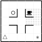
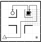
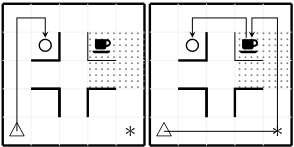
To illustrate our problem, we consider a simple stochastic office world environment, adapted from [Camacho et al., 2019], shown in Figure 1. The environment consists of three features: office ◦, coffee coffee, and decoration ∗. A slippery area (shaded) near the coffee station introduces randomness in the agent's movement. In this environment, desirable and undesirable strategies correspond to positive and negative DTMCs, respectively. Based on this input, a possible formula
(a) Office-world environment
Positive example
Negative examples
(b) Strategies in the environment
Figure 1: An illustration of an office-world environment with the following features: office ◦, coffee coffee, and decoration ∗. The shaded part near coffee is slippery and introduces stochasticity in the agent's movement. The positive example demonstrates a strategy where the agent △ collects coffee and delivers to ◦ while avoiding ∗, whereas the negative examples do not achieve this temporal task.
could be P≥0.9[F(coffee ∧ F(◦))] ∧ P≥0.9[G(¬∗)], which is a conjunction of two PLTL formulas. This formula uses the temporal operators F (eventually) and G (always), along with the probabilistic quantifier P≥0.9 (at least 0.9 probability) to state that the agent has a high probability of getting coffee and delivering it to the office while avoiding the decoration.
To address the passive learning problem for PLTL, we propose a novel symbolic search algorithm comprising three key procedures. The first procedure uses grammar-based enumeration to identify candidate LTL formulas. The second procedure determines threshold values for probabilistic quantifiers through probabilistic model checking, which results in a PLTL formula. Finally, the third procedure constructs Boolean combinations of PLTL formulas using a generalization of the set-cover problem.
To improve learning, the algorithm incorporates several heuristics for pruning the search space, including LTL simplification rules, inference techniques based on model checking, and tactics for Boolean combinations. Overall, the algorithm is designed with theoretical guarantees to learn concise and interpretable PLTL formulas from DTMCs.
We implement our algorithm as a tool PriTL to leverage the grammar-based search heuristic coupled with the state-ofthe-art tool PRISM [Kwiatkowska et al., 2011] for probabilistic model checking of DTMCs. We evaluate PriTL through two case studies. In the first case study, we consider learning PLTL formulas to distinguish between desirable and undesirable strategies obtained using RL for a variety of temporal tasks. In the second case study, we consider distinguishing between different variants of a probabilistic protocol. In both case studies, PriTL effectively infers concise and descriptive PLTL formulas that explain the probabilistic temporal behaviour of the systems. Moreover, we demonstrate how the different procedures contribute to the learning process. We refer the reader to the extended version [Roy et al., 2025] for additional proofs, implementation details, and experimental results.
1.1 RelatedWork
There are two main areas of related work: learning temporal logics from data and explaining strategies/policies in RL.
Learning Temporal Logics. There are numerous works on learning temporal logics from data, specifically focusing on LTL [Neider and Roy, 2025] and STL [Bartocci et al.,
2022]. Our work falls within the category of exact learning, which seeks to infer minimal formulas that perfectly fit the data with provable guarantees. Notable works in this category include those for LTL [Neider and Gavran, 2018; Camacho and McIlraith, 2019; Raha et al., 2022; Valizadeh et al., 2024], STL [Mohammadinejad et al., 2020], and several other temporal logics such as PSL [Roy et al., 2020], CTL [Pommellet et al., 2024] and ATL [Bordais et al., 2024]. The learning techniques primarily involve deductive methods such as constraint solving and enumerative search.
There are also several works within the category of approximate learning, which seeks to infer formulas that fit (typically noisy) data well. Notable works in this category include those for LTL [Bartocci et al., 2014; Luo et al., 2022; Wan et al., 2024; Chiariello, 2024] and STL [Nenzi et al., 2018]. The learning techniques involve statistical optimisation, genetic algorithms, and neural network inference.
Our work considers the exact learning of probabilistic LTL, which, to our knowledge, has not been explored before. Moreover, we introduce a new learning framework based on symbolic search guided by dedicated model checkers.
Explaining RL policies Several approaches exist for explaining policies in reinforcement learning [Milani et al., 2024]. Our work falls within the category of global explanations of pre-trained policies using formal languages. Notable works in this category include providing contrastive explanation using restricted queries in PCTL * [Boggess et al., 2023], extracting finite-state machines from neural policies [Danesh et al., 2021], and summarizing using abstract policy graphs [Topin and Veloso, 2019].
In contrast, our approach explains the temporal difference between policies using the full expressive power of PLTL. Such explanations can also be translated to natural language [Fuggitti and Chakraborti, 2023].
2 Preliminaries
Let N = {0, 1, 2, . . . } be the set of natural numbers.
2.1 Markov Chains andMDPs
A discrete-time Markov chain (DTMC) is a tuple M = (S, sI, P,AP, ℓ), where S is a finite set of states, sI ∈ S is an initial state, P : S×S ↦→ [0, 1] is a probabilistic transition function, AP is a set of atomic propositions and ℓ : S ↦→ 2AP
is a labelling function. Atomic propositions will form the basis for temporal logic specifications and the function l defines the propositions that are true in each state.
A path π of M is an infinite sequence of states π = s0s1s2 . . . ∈ Sω such that P(si, si+1) > 0 for all i ∈ N. We denote the state at position i of a path π by π[i] = si and the infinite suffix starting in π[i] as π[i :] = sisi+1 . . . . The set of all paths of M starting from state s is written as ΠM (s). In standard fashion [Kemeny et al., 1976], we define a probabilitymeasure PrMs on the set of infinite paths ΠM (s). A Markov decision process (MDP) is a tuple (S, sI,A, P,AP, ℓ), which extends a DTMC by allowing a choice between actions in each state. The set of all actions is A and the probabilistic transition function becomes P : S × A × S ↦→ [0, 1], where P(s, a, s′ ) is the probability to move to s′ when action a is taken in s.
A strategy (a.k.a., policy) of an MDP defines which action is taken in each state, based on the history so far. In their most general form, strategies are defined as functions σ : (S × A)∗S ↦→ ∆(A), where ∆(A) is the set of distributions over A. The behaviour of an MDP under a strategy σ is defined by an induced DTMC, which we denote by M σ . In general, M σ is infinite state. In this paper, however, we can restrict to finite-memory strategies, whose action choices depend only on the current state and a finite set of memory values, since these suffice for objectives specified in LTL. In this case, the induced DTMCM σ is finite [Baier and Katoen, 2008].
2.2 Probabilistic Linear Temporal Logic (PLTL)
Probabilistic Linear Temporal Logic (PLTL) is the probabilistic variant of the popular logic LTL, and is commonly used to express the temporal behaviour of probabilistic systems. A PLTL formula takes the form P▷◁p[φ], stating that the probability with which LTL formula φ is satisfied meets the probability threshold ▷◁ p. For example, PLTL formula P≥0.9[F(a ∧ Fb)] means that the probability of observing proposition a and then b is at least 0.9.
In this work, we learn specifications expressed in an extension of PLTL, which we call PLTL+, that allows positive Boolean combinations of PLTL formulas.
Formally, the syntax and semantics of these logics are defined as follows. Firstly, LTL formulas φ are defined inductively using the following grammar:
where p ∈ AP is an proposition, ¬ (not), ∨ (or) and ∧ (and) are standard Boolean operators, and X (neXt), U (Until) are standard temporal operators. We allow the standard temporal operators F (Finally) and G (Globally) as syntactic sugar, where Fφ := true Uφ and Gφ := ¬F¬φ.
We interpret LTL formulas over paths of a DTMC. The satisfaction of LTL formula φ by (infinite) path π is defined inductively as follows:
We interpret Boolean combinations in the standard fashion and therefore omit the definitions.
A PLTL+ formula Φ is defined as:
where ▷◁ ∈ {<, >, ≤, ≥}, p ∈ [0, 1] is a probability threshold and φ is an LTL formula.
A PLTL+ (or PLTL) formula is interpreted over the states of a DTMC. The satisfaction of PLTL+ formula Φ by a state s is defined as follows:
where PrM (s |= φ) = PrMs ({π ∈ ΠM (s) | π |= φ}) denotes the probability that LTL formula φ is satisfied by a path starting in state s of M. We say that a DTMC M satisfies a PLTL+ formula Φ if, for the initial state sI of M, sI |= Φ.
3 Passive Learning of PLTL+ Formulas
We frame the problem of learning a PLTL+ formula as a typical passive learning problem [Gold, 1978]. Apart from being a fundamental learning problem, passive learning forms a key subroutine in other learning frameworks, such as active learning [Camacho and McIlraith, 2019] and learning from positive examples [Roy et al., 2023].
In this problem, we rely on a sample S = (P,N) consisting of a set P of positive DTMCs and a set N of negative DTMCs. We define sample size |S| as the total number of DTMCs in S. The goal is to learn a concise PLTL+ formula Φ that is consistent with S = (P,N), i.e., for all M ∈ P , M |= Φ, and for all M ∈ N, M ̸|= Φ.
To quantify conciseness, we measure the size |Φ| of PLTL+ formulas Φ. To avoid checking redundant formulas, our learning algorithm uses LTL in negation normal form (NNF), a standard syntactic form where negation applies only to atomic propositions. We define the size of an LTL formula by the number of operators ◦ ∈ {F,X,G,U, ∧, ∨} and literals Λ = {p, ¬p | p ∈ AP} in the formula. For instance, the formula F(p ∧ F(¬q)) has size 5. The size of a PLTL+ formula Φ is defined exactly the same way.
We now formally define the problem of passive learning of PLTL formulas.
Problem 1. Given a sample S = (P,N), size bound K and propositions AP, learn a minimal PLTL+ formula Φ over AP such that: (i) Φ is consistent with S, and (ii) |Φ| ≤ K.
A solution to Problem 1 (which is not necessarily unique) is a concise PLTL+ formula Φ that distinguishes between the probabilistic temporal behaviour of the positive and negative DTMCs. The size bound K ensures three attributes for the solution formula Φ: (i) it does not get too large, (ii) it does not overfit to the sample, and (iii) it makes the passive learning problem decidable, ensuring a terminating algorithm.
4 The Learning Algorithm
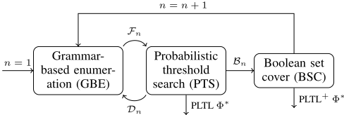
We now describe the learning algorithm that we propose to solve Problem 1. Figure 2 provides a high-level overview of our algorithm. The algorithm consists of three main procedures: (i) grammar-based enumeration, which efficiently enumerates through the space of LTL formulas, (ii) probabilistic threshold search, which employs probabilistic model checking to determine whether a formula is consistent with the given sample, and (iii) Boolean set cover, which constructs Boolean combinations of PLTL formulas to form a consistent formula. The algorithm iterates over formulas of increasing size, starting from 1, using GBE, and then checks the consistency of the formulas using PTS and BSC. We now describe each of these procedures in detail.
4.1 Grammar-based Enumeration for LTL
The grammar-based enumeration (GBE) procedure incrementally explores the space of LTL formulas. Since the number of syntactically distinct formulas grows exponentially with formula size 1 , GBE employs pruning techniques to manage the search space efficiently.
Importantly, GBE relies on the nesting depth (or depth, for brevity) of temporal operators in formulas. We define the nesting depth d(φ) for LTL recursively as: d(l) = 0 for l ∈ Λ, d(φ ◦ φ′ ) = max(d(φ), d(φ′ )) for ◦ ∈ {∧, ∨}, d(◦φ) = 1 + d(φ) for ◦ ∈ {X, F, G}, d(φUφ′ ) = 1+max(d(φ), d(φ′ )). For instance, the formula F(p ∧ F(¬q)) has depth 2.
The nesting depth is essential for managing the search space effectively as well as ensuring the practical applicability of the formulas. Heavily nested formulas (e.g., those with a depth > 3) are considered hard to interpret [Camacho and McIlraith, 2019] and are also uncommon in widely used LTL patterns [Dwyer et al., 1998]. Therefore, GBE incorporates maximum depth D as a parameter.
To build formulas Fn of size n and all depths d ≤ D, GBE employs a bottom-up dynamic programming approach. Specifically, the set Fn is built as a union of subsets F d n of LTL formulas of size n and depth d. GBE initializes F 0 1 := Λ and F d 1 := ∅ for 0 < d ≤ D. It then inductively combines formulas fromF d n of different depths to form larger formulas.
The inductive step of GBE Fn+1 is outlined in Algorithm 1. It follows the LTL grammar, adding operators to smaller formulas to construct larger ones. The algorithm uses two heuristics to eliminate semantically equivalent (≡) formulas, where φ ≡ φ′ if and only if π |= φ ↔ π |= φ′ for any path π ∈ (2AP)ω . These heuristics are briefly described here.
1 Asymptotically 7n√14 2√πn3 [Flajolet and Sedgewick, 2009]
Algorithm 1 Inductive step in GBE
Input: Fn, Max depth D 1: for d = 0 to D do 2: F d n+1 = ∅ 3: for φ ∈ F d-1 n do 4: Construct ψ = ◦φ for ◦ ∈ {X,F,G} 5: Add ψ to F d n+1 if temporal simplify does not hold 6: end for 7: for k = 1 to n - 1 do 8: for φ ∈ F d-1 k and φ′ ∈ ⋃d′<d F d′ n-k do 9: ψ = φUφ′ 10: Add ψ to F d n+1 if Boolean simplify does not hold 11: end for 12: for φ ∈ F d k and φ′ ∈ ⋃d′≤d F d′ n-k do 13: ψ = φ ◦ φ′ for ◦ ∈ {∧, ∨} 14: Add ψ to F d n+1 if Boolean simplify does not hold 15: end for 16: end for 17: end for 18: return Fn+1The first heuristic, temporal simplification, removes redundant formulas by applying syntactic rules to rewrite LTL formulas into normal forms [Baier and Katoen, 2008, Fig. 5.7]. For example, FF(p) ≡ F(p), FX(p) ≡ XF(p), and FGF(p) ≡ GF(p) (see [Duret-Lutz, 2024, Sec. 5.4] for the full list). If a constructed formula is not in simplified form, it is discarded. These checks are constant-time operations, making them highly efficient.
The second heuristic, Boolean simplification, removes redundant Boolean combinations such as φ1 ∧ φ2 or φ1 ∨ φ2, where φ1 ≡ φ2 or φ1 ≡ ¬φ2. It checks the syntactic equality of φ1 and φ2 via a linear-time scan of their syntax trees. It then checks semantic equivalence, which can be doubly exponential in formula size but is efficiently handled by modern LTL satisfiability checkers [Duret-Lutz et al., 2022].
We formalise the completeness of the GBE procedure below 2 , which can be proved by induction on formula size.
Lemma 1. ⋃n≤N ′ Fn computed by GBE consists of all semantically distinct formulas of size ≤ N ′ and depth ≤ D.
4.2 Probabilistic Threshold Search for PLTL
The probabilistic threshold search (PTS) procedure steps through the formulas generated by GBE and evaluates the likelihood of the formulas being satisfied/consistent. The main steps of PTS are outlined in Algorithm 2.
PTS first computes the probability measure for a formula φ ∈ Fn for each M in the given sample. More specifically, PTS computes the vector V M,φ : S → [0, 1], mapping each state s ∈ S of M to PrM (s |= φ). We use vM,φ I = V M,φ(sI) to denote the probability for the initial state sI of M.
Our implementation, which is based on the PRISM tool [Kwiatkowska et al., 2011], deploys standard probabilistic LTL model checking procedures [Baier and Katoen, 2008]. First, the LTL formula φ is translated into an equivalent deterministic Rabin automaton (DRA) Aφ. Then the product DTMC M × Aφ, which combines the DTMC and DRA, is constructed and solved using standard numerical methods based on value iteration.
2 This result establishes GBE's complete search in isolation; when combined with PTS, as we see later in Section 4.2, several formulas are pruned using heuristics.
PTS exploits the computed vector V M,φ to search for a formula that has a higher probability of satisfaction in the positive examples than in the negative examples. For this, it computes the minimum probability pφ = min{vM,φ I | M ∈ P} of satisfaction of φ among the samples in the set P, and the maximum probability nφ = max{vM,φ I | M ∈ N} of satisfaction of φ among the samples in the set N.
To identify a significant probabilistic difference in the temporal behaviour, PTS employs a small tolerance parameter δ ∈ (0, 0.1). We explain the motivation for this parameter using the introductory example from Figure 1. In this example, the probability of reaching the office, i.e., satisfying F(◦), can be slightly lower in the positive example (say 0.94) compared to the negative examples (say, 1.0 and 0.95). This small difference could arise because the agent takes a slightly longer slippery route in the positive example than in the second negative example. However, F(◦) is not a primary distinguishing factor between the positive and negative examples and must not be considered by PTS.
Thus, PTS checks if the difference pφ - nφ between the probability of satisfaction of φ in the positive and negative examples is greater than the tolerance δ. If indeed pφ-nφ > δ, then PTS outputs the formula Φ = P>mφ [φ], where the threshold mφ = pφ+nφ 2 . While any threshold between pφ and nφ could be chosen, the choice of the mean of the two values is to reduce overfitting to the input sample.
We state the soundness of the PTS procedure as follows.
Lemma 2. If PTS returns a PLTL formula Φ, then Φ is consistent with sample S.
Proof. PTS always returns a formula of the form Φ = P>mφ [φ], where mφ = pφ+nφ 2 and pφ - nφ > δ. We can state that
Note that PTS restricts the search to only PLTL formulas of the form P>p[φ]. The relation ≥ is not required due to the non-zero parameter δ, while the < relation can be derived from the > relation and the dual LTL formula ¬φ using the relation P<p[φ] ≡ P>1-p[¬φ].
If a formula φ is not consistent, PTS discards it by adding it to Dn if it is not useful for the next GBE iterations; otherwise, it adds φ to Bn for Boolean combinations. We briefly discuss the heuristics used for discarding formulas.
This heuristic, inconsistency removal, discards φ if the following condition holds: V M,φ ≡ 0 for each M ∈ P, or V M,φ ≡ 1 for each M ∈ N, where 0 and 1 are the vectors with all zeros and all ones, respectively. In simpler terms, φ is discarded if it is unsatisfiable in any state of the positive
Algorithm 2 Probabilistic Threshold Search (PTS)
Input: Fn, Probabilistic tolerance δ
- 1: for d = 0 to D, φ ∈ F d n do
- 2: Compute V M,φ for eachM in S
- 3: pφ = min M∈P {vM,φ I }, nφ = max M∈N {vM,φ I }
- 4: if pφ - nφ > δ then
- 5: return Φ = P> pφ+nφ 2 [φ]
- 6: else
- 7: Add φ to Dn if inconsistency removal holds
- 8: Add φ to Bn otherwise
- 9: end if
- 10: end for
DTMCs or universally satisfied in all states of the negative DTMCs. Such formulas cannot be meaningfully combined in subsequent iterations, as stated below for the positive cases; a similar argument applies to the negative cases.
Lemma 3. Let V M,φ ≡ 0 for each M ∈ P. Then φ cannot be a subformula of a minimal consistent PLTL formula.
Examples of formulas that can be discarded from the introductory example include F(∗ ∧ coffee), G(coffee), and G(∗) since they never hold in any state of the positive DTMC.
4.3 Boolean Set Cover for PLTL+
The Boolean Set Cover (BSC) procedure combines PLTL formulas using Boolean operations. We adapt this procedure, originally introduced in [Raha et al., 2022], to accommodate probability thresholds. The steps of our algorithm are detailed in Algorithm 3.
First, BSC discards formulas from Bn that are not useful for Boolean combinations. For this, it uses a condition similar to, but weaker than, inconsistency removal used in PTS: vM,φ I = 0 for all M ∈ P, or vM,φ I = 1 for all M ∈ N.
For the remaining formulas, BSC assesses how close they are to being a consistent formula. To do this, it relies on the function c(φ, r), which quantifies the quality of φ with probability threshold r, defined as follows:
where �·� denotes the Iverson bracket, evaluating to 1 if the condition holds, and 0 otherwise. We have c(φ, r) = |S| if and only if P>r[φ] is consistent with S.
BSC computes, for each LTL formula φ ∈ Bn, a maximal probability threshold r∗ = argmaxr∈(0,1) c(φ, r) that maximizes consistency with S. This can be computed via a linear scan over the sorted list of probabilities vM,φ I for M in S.
BSC then constructs the PLTL formula Φ = P>r∗ [φ] along with its score σ(Φ) = c(φ, r∗ )/(1 + √|Φ|) and adds it to a heap H. The scoring function and the subsequent steps of BSC are as in [Raha et al., 2022]. Briefly, a maximum Boolean combination limit L is considered. The PLTL formulas with the L highest scores are selected, and combined as disjunctions and conjunctions with all formulas in H.
Below, we state the soundness of BSC for PLTL, based on [Raha et al., 2022].
Input: Bn, Max size K, Max Limit L 1: Discard formulas fromBn not suitable for bool comb 2: for φ ∈ Bn do 3: Compute Φ = P>r∗[φ], score σ(Φ) and add to H 4: end for 5: H∗ ← Highest L formulas in H w.r.t score σ 6: for Ψ ∈ H and Φ ∈ H∗ do 7: Φ′ := Ψ ◦ Φ for ◦ ∈ {∧, ∨} 8: if |Φ′ | ≤K and Φ′ is consistent then 9: Store Φ′ as consistent and update K ← |Φ′ | - 1 10: end if 11: end forLemma 4. If BSC returns a PLTL+ formula Φ, then Φ is consistent with sample S.
Theoretical guarantees. We state the guarantees of our algorithm with respect to the search space Θ(K, D, δ) of PLTL formulas constrained by the considered parameters, i.e., size ≤ K, depth ≤ D and tolerance > δ.
Theorem 1. Given sample S, size K, depth D, and tolerance δ, our learning algorithm has the following guarantees:
- (soundness) if it returns a PLTL+ formula Φ, then Φ is consistent with S and |Φ| ≤ K, and
- (completeness andminimality) if there exists a PLTL formula in Θ(K,D, δ) consistent with S, then it returns a minimal PLTL+ formula.
Proof. Soundness follows from the correctness of PTS (Lemma 2) and BSC (Lemma 4) in outputting a consistent formula. Completeness is ensured by the exhaustive enumeration by GBE (Lemma 1), discarding only inconsistent formulas (Lemma 3). Minimality follows from the complete iterative search over increasing formula sizes (see Fig. 2).
5 Evaluation
In this section, we evaluate the capability of our learning algorithm to infer concise PLTL+ formulas from samples of DTMCs. To this end, we developed a prototype tool, PriTL 3 , implemented in Python3, which integrates the three procedures, GBE, PTS and BSC, of the learning algorithm. For heuristics in GBE, we rely on LTL simplification and satisfaction features from the SPOT library [Duret-Lutz et al., 2022]. For LTL model checking of DTMCs in PTS, we rely on the PRISM tool [Kwiatkowska et al., 2011], using its (default) hybrid model checking engine.
To the best of our knowledge, no existing tool can directly learn arbitrary temporal specifications fromDTMCs. To evaluate PriTL's ability to learn concise and distinguishing formulas, we tested it on strategies generated within a stochastic environment and on various variants of a probabilistic model. For all experiments, we set the maximum depth D = 2, tolerance δ = 0.05, and a Boolean combination limit L = 10. If PriTL identifies multiple minimal formulas, it returns the one with the highest probability difference, pφ - nφ. In case of a tie, PriTL returns all valid formulas.
3 https://github.com/rajarshi008/PriTL
We conducted all experiments on a MacBook Pro M3 (macOS 14.6.1) with 18 GB RAM. A detailed discussion of the implementation and experiments can be found in the appendix of the extended version [Roy et al., 2025].
Learning from strategies in stochastic environment
For this experiment, we focus on strategy DTMCs generated via non-Markovian reinforcement learning algorithms. Specifically, we utilize different Q-learning algorithms proposed by [Shao and Kwiatkowska, 2023] that are capable of generating optimal strategies for LTL tasks.
As the underlying MDP, we select the widely used OpenAI Gym frozen lake environment [Brockman et al., 2016], employing the same layout as in [Shao and Kwiatkowska, 2023]. This environment is an 8×8 gridworld, where an agent navigates a slippery frozen lake, introducing stochasticity: with a 1/3 probability, the agent moves in the intended direction, and with a 1/3 probability, it deviates sideways. The environment includes three key features: two campsites, a and b, and several holes h.
We evaluate PriTL on two distinct applications: (i) learning from strategies trained on correct and incorrect LTL tasks, and (ii) learning from optimal and suboptimal strategies for the same LTL task. For both (i) and (ii), we set the propositions AP = {a, b, h} and formula size bound K = 10.
For application (i), we identify several desirable LTL tasks and designate them as correct tasks. As incorrect tasks, we select LTL tasks that are less precise than their correct counterparts. For example, the correct task F(a)∧G(¬h) requires reaching campsite a while always avoiding holes h, whereas the incorrect task F(a) specifies a weaker condition of reaching the campsite, which may result in falling into holes. The first two columns of Table 1 list the considered correct and incorrect tasks, respectively. For each correct and incorrect task, we generate 10 positive and 10 negative optimal strategy DTMCs, respectively, using the CF+KC Q-learning algorithm [Shao and Kwiatkowska, 2023], known for its fast convergence to optimality. The cumulative state space of the samples is of the order of 103 (see fourth column of Table 1).
We present the learned PLTL+ formulas for each task in Table 1. For the first two tasks, PriTL inferred PLTL+ formulas with safety properties, G(¬h) and ¬hUa, which were violated in the negative examples. In subsequent tasks, PriTL inferred formulas that indicate the specific requirements missing in the negative examples. These include repeated reachability GF(a) instead of simple reachability F(a), performing two tasks simultaneously F(a) ∧ F(b) instead of just one F(a) or F(b), etc. Overall, PriTL successfully produced concise formulas that explain the differences between strategies trained on different tasks.
For application (ii), we identify some more desirable LTL tasks (in Figure 3) and generate optimal and suboptimal strategies for each. We extract strategy DTMCs from intermediate episodes of the KC Q-learning algorithm since it has relatively slower convergence to optimality [Shao and Kwiatkowska, 2023], thereby often yielding sub-optimal strategies. We considered a strategy that achieves a high probability (i.e., p ≥ 0.95) as optimal, while one that achieves a lower probability (i.e., 0.5 ≤ p ≤ 0.9) as suboptimal. Overall, for each LTL task, we collected at least 30 positive DTMCs and 30 negative DTMCs corresponding to optimal and suboptimal strategies, respectively. We evaluated our algorithm using varying sample sizes |S|, ranging from 10 to 60 DTMCs per sample, with an equal split between positive and negative examples.
| Correct task for P | Incorrect task(s) for N | Learned PLTL+ Formula | State space S LTL Space | Time (sec) | |
|---|---|---|---|---|---|
| F(a) ∧ G(¬h) | F(a) | P>0.76[G(¬h)] | 2.5 · 103 | 24/24 | 1.77 |
| F(a) ∧ G(¬h) | F(a), G(¬h) | P>0.76[¬h U a] | 1.9 · 103 | 110/186 | 3.39 |
| F G(a) ∧ G(¬h) | F(a) ∧ G(¬h) | P>0.49[FG(a)], P>0.49[GF(a)] | 2.7 · 103 | 112/186 | 4.93 |
| G F(a) ∧ G F(¬a) ∧ G(¬h) | F G(a) ∧ G(¬h) | P>0.5[G F(¬a)] | 0.9 · 103 | 50/186 | 3.9 |
| F(a) ∧F(b) ∧G(¬h) | F(a) ∧G(¬h), F(b) ∧G(¬h) | P>0.5[F(a)] ∧P>0.99[F(b)] | 3.2 · 103 | 476/7314 | 24.1 |
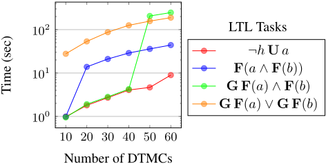
We present the runtime for varying sample sizes in Figure 3. For the tasks ¬hUa and GF(a) ∨ GF(b), PriTL consistently inferred the formulas P>0.9[G(¬h)] and P>0.93[GF(a) ∨ GF(b)], respectively, across all samples. The runtime for these increased linearly with the sample size.
For the task F(a ∧ F(b)), PriTL inferred P>0.97[F(b)] for a sample size of 10 and a more precise formula, P>0.94[F(a)] ∧ P>0.97[F(b)], for larger sizes. Similarly, for the task GF(a) ∧ F(b), PriTL inferred P>0.92[F(b)], for smaller samples (≤ 40), whereas it inferred a more precise formula, P>0.92[GF(a)] ∧ P>0.95[F(b)] for larger samples (50 and 60). Both tasks showed a runtime spike due to the change in the inferred formula, deviating from the linear trend in other tasks. Moreover, in both cases, the more precise formula was inferred by the BSC procedure. Overall, PriTL successfully inferred expected PLTL+ formulas, with runtime generally scaling linearly with sample size.
We also briefly discuss how different parts of PriTL contribute to the learning process. PTS dominates the running time, while GBE and BSC take negligible time. For example, inferringP>0.5[F(a)]∧P>0.99[F(b)] (fromTable 1) took 24.05 seconds for PTS, and 0.05 and 0.01 seconds for GBE and BSC, respectively. The heuristics enhance efficiency by reducing the search space, particularly for larger formulas. The fifth column of Table 1 compares the considered formula for PTS with the total space up to the size of the learned formula. For the same example, the search was reduced to just 7% of the possible LTL space via heuristics.
Learning from variants of probabilistic models
In this experiment, we compare two implementations of the probabilistic secret-sharing protocol EGL [Even et al., 1985; Norman and Shmatikov, 2006], where two parties, A and B, share 2P secrets (2-length bit-vectors) over several rounds. The two implementations we consider, EGL1P and EGL2P , are parametrized by the number of secrets P = 1, . . . , 7. The key difference in the variants is in the sharing order: in EGL1P , each party sequentially shares all their ith bits, while in EGL2P , they alternately share half of their ith bits.
To apply PriTL, we treat EGL1P as positive, EGL2P as negative, K = 6 and AP = {kA, kB}, where kA (kB resp.) represents A (B resp.) knows of B's (A's resp.) secrets.
For P = 1, 2, 3, 4, 5, PriTL inferred the formula P>p[¬kAUkB] with progressively increasing thresholds p = 0.88, 0.90, 0.94, 0.97 with running times 0.37, 0.38, 0.68, 1.31 seconds, respectively. The inferred formula indicates that, in EGL1P , the probability that B knows A's secret before A knows B's is higher as compared to EGL2P .
For P > 5, however, PriTL did not infer any formula. This indicates that no PLTL formula with parameters K ≤ 6, d ≤ 2 and δ > 0.05 distinguishes the variants when a higher number of secrets are shared, based on our exhaustive search (Theorem 1). Overall, PriTL could identify key probabilistic temporal differences between variants of probabilistic models, or confirm their absence.
6 Conclusion
We focused on the automatic learning of temporal behaviour in stochastic systems. Specifically, we considered the passive learning problem of learning concise probabilistic LTL (PLTL) formulas that distinguish between positive and negative Markov chains. Our novel learning algorithm combines grammar-based enumeration with probabilistic model checking, enhanced by search heuristics. We demonstrated the ability of our approach in inferring temporal specifications in both reinforcement learning and modelling applications.
In the future, we plan to integrate our algorithm into other learning frameworks, such as active learning [Camacho and McIlraith, 2019] and learning from positive examples [Roy et al., 2023]. Moreover, we aim to extend our approach to multi-agent systems [Boggess et al., 2023].
Acknowledgements
This project received funding from the ERC under the European Union's Horizon 2020 research and innovation programme (grant agreement No.834115, FUN2MODEL). The work was done while YP visited the University of Oxford for an internship.
@inproceedings{ijcai2025p517,
  title     = {Learning Probabilistic Temporal Logic Specifications for Stochastic Systems},
  author    = {Roy, Rajarshi and Pote, Yash and Parker, Dave and Kwiatkowska, Marta},
  booktitle = {Proceedings of the Thirty-Fourth International Joint Conference on
               Artificial Intelligence, {IJCAI-25}},
  publisher = {International Joint Conferences on Artificial Intelligence Organization},
  editor    = {James Kwok},
  pages     = {4642--4650},
  year      = {2025},
  month     = {8},
  note      = {Main Track},
  doi       = {10.24963/ijcai.2025/517},
  url       = {https://doi.org/10.24963/ijcai.2025/517},
}
TY - CPAPER TI - Learning Probabilistic Temporal Logic Specifications for Stochastic Systems AU - Roy, Rajarshi AU - Pote, Yash AU - Parker, Dave AU - Kwiatkowska, Marta T2 - Proceedings of the Thirty-Fourth International Joint Conference on Artificial Intelligence, IJCAI-25 PB - International Joint Conferences on Artificial Intelligence Organization PY - 2025 SP - 4642 EP - 4650 DO - 10.24963/ijcai.2025/517 UR - https://doi.org/10.24963/ijcai.2025/517 ER -Copied
Machine-readable versions of this paper, for tools and AI agents:





