
Explainable Graph Neural Networks via Structural Externalities
Proceedings of the Thirty-Fourth International Joint Conference on Artificial Intelligence. Main Track. Pages 583-591.
https://doi.org/10.24963/ijcai.2025/66
Keywords
- AI Ethics, Trust, Fairness: ETF: Explainability and interpretability
Abstract
Graph Neural Networks (GNNs) have achieved outstanding performance across a wide range of graph-related tasks. However, their "black-box" nature poses significant challenges to their explainability, and existing methods often fail to effectively capture the intricate interaction patterns among nodes within the network. In this work, we propose a novel explainability framework, GraphEXT, which leverages cooperative game theory and the concept of social externalities. GraphEXT partitions graph nodes into coalitions, decomposing the original graph into independent subgraphs. By integrating graph structure as an externality and incorporating the Shapley value under externalities, GraphEXT quantifies node importance through their marginal contributions to GNN predictions as the nodes transition between coalitions. Unlike traditional Shapley value-based methods that primarily focus on node attributes, our GraphEXT places greater emphasis on the interactions among nodes and the impact of structural changes on GNN predictions. Experimental studies on both synthetic and real-world datasets show that GraphEXT outperforms existing baseline methods in terms of fidelity across diverse GNN architectures , significantly enhancing the explainability of GNN models.
- [Baldassarre and Azizpour, 2019] Federico Baldassarre and Hossein Azizpour. Explainability techniques for graph convolutional networks. arXiv preprint arXiv:1905.13686, 2019.
- [Funke et al., 2022] Thorben Funke, Megha Khosla, Man- deep Rathee, and Avishek Anand. Zorro: Valid, sparse, and stable explanations in graph neural networks. IEEE Transactions on Knowledge and Data Engineering, 35(8):8687-8698, 2022.
- [Gao and Ji, 2019] Hongyang Gao and Shuiwang Ji. Graph u-nets. In international conference on machine learning, pages 2083-2092. PMLR, 2019.
- [Gui et al., 2023] Shurui Gui, Hao Yuan, Jie Wang, Qicheng Lao, Kang Li, and Shuiwang Ji. Flowx: Towards ex- plainable graph neural networks via message flows. IEEE Transactions on Pattern Analysis and Machine Intelli- gence, 2023.
- [Huang et al., 2022] Qiang Huang, Makoto Yamada, Yuan Tian, Dinesh Singh, and Yi Chang. Graphlime: Local in- terpretable model explanations for graph neural networks. IEEE Transactions on Knowledge and Data Engineering, 35(7):6968-6972, 2022.
- [Kipf and Welling, 2016] Thomas N Kipf and Max Welling. Semi-supervised classification with graph convolutional networks. arXiv preprint arXiv:1609.02907, 2016.
- [Kuhn and Tucker, 1953] Harold William Kuhn and Al- bert William Tucker. Contributions to the Theory of Games. Number 28. Princeton University Press, 1953.
- [Liu et al., 2021] Meng Liu, Youzhi Luo, Limei Wang, Yaochen Xie, Hao Yuan, Shurui Gui, Haiyang Yu, Zhao Xu, Jingtun Zhang, Yi Liu, et al. Dig: A turnkey library for diving into graph deep learning research. Journal of Machine Learning Research, 22(240):1-9, 2021.
- [Luo et al., 2020] Dongsheng Luo, Wei Cheng, Dongkuan Xu, Wenchao Yu, Bo Zong, Haifeng Chen, and Xiang Zhang. Parameterized explainer for graph neural net- work. Advances in neural information processing systems, 33:19620-19631, 2020.
- [Macho-Stadler et al., 2007] Inés Macho-Stadler, David Pérez-Castrillo, and David Wettstein. Sharing the surplus: An extension of the shapley value for environ- ments with externalities. Journal of Economic Theory, 135(1):339-356, 2007.
- [Myerson, 1977] Roger B Myerson. Graphs and cooperation in games. Mathematics of operations research, 2(3):225- 229, 1977.
- [Navarro, 2007] Noemí Navarro. Fair allocation in net- works with externalities. Games and Economic Behavior, 58(2):354-364, 2007.
- [Pope et al., 2019] Phillip E Pope, Soheil Kolouri, Moham- mad Rostami, Charles E Martin, and Heiko Hoffmann. Ex- plainability methods for graph convolutional neural net- works. In Proceedings of the IEEE/CVF conference on computer vision and pattern recognition, pages 10772- 10781, 2019.
- [Skibski et al., 2013] Oskar Skibski, Tomasz P Michalak, and Michael Wooldridge. The shapley axiomatization for values in partition function games. arXiv preprint arXiv:1308.6255, 2013.
- [Springenberg et al., 2014] Jost Tobias Springenberg, Alexey Dosovitskiy, Thomas Brox, and Martin Ried- miller. Striving for simplicity: The all convolutional net. arXiv preprint arXiv:1412.6806, 2014.
- [Veličković et al., 2017] Petar Veličković, Guillem Cucurull, Arantxa Casanova, Adriana Romero, Pietro Lio, and Yoshua Bengio. Graph attention networks. arXiv preprint arXiv:1710.10903, 2017.
- [Wu et al., 2018] Zhenqin Wu, Bharath Ramsundar, Evan N Feinberg, Joseph Gomes, Caleb Geniesse, Aneesh S Pappu, Karl Leswing, and Vijay Pande. Moleculenet: a benchmark for molecular machine learning. Chemical sci- ence, 9(2):513-530, 2018.
- [Xu et al., 2018] Keyulu Xu, Weihua Hu, Jure Leskovec, and Stefanie Jegelka. How powerful are graph neural net- works? arXiv preprint arXiv:1810.00826, 2018.
- [Yang et al., 2021] Yaming Yang, Ziyu Guan, Jianxin Li, Wei Zhao, Jiangtao Cui, and Quan Wang. Interpretable and efficient heterogeneous graph convolutional network. IEEE Transactions on Knowledge and Data Engineering, 35(2):1637-1650, 2021.
- [Ying et al., 2019] Zhitao Ying, Dylan Bourgeois, Jiaxuan You, Marinka Zitnik, and Jure Leskovec. Gnnexplainer: Generating explanations for graph neural networks. Ad- vances in neural information processing systems, 32, 2019.
- [Yuan et al., 2020] Hao Yuan, Jiliang Tang, Xia Hu, and Shuiwang Ji. Xgnn: Towards model-level explanations of graph neural networks. In Proceedings of the 26th ACM SIGKDD international conference on knowledge discov- ery & data mining, pages 430-438, 2020.
- [Yuan et al., 2021] Hao Yuan, Haiyang Yu, Jie Wang, Kang Li, and Shuiwang Ji. On explainability of graph neural networks via subgraph explorations. In International con- ference on machine learning, pages 12241-12252. PMLR, 2021.
- [Yuan et al., 2022] Hao Yuan, Haiyang Yu, Shurui Gui, and Shuiwang Ji. Explainability in graph neural networks: A taxonomic survey. IEEE transactions on pattern analysis and machine intelligence, 45(5):5782-5799, 2022.
- [Zeiler and Fergus, 2014] Matthew D Zeiler and Rob Fergus. Visualizing and understanding convolutional networks. In Computer Vision-ECCV 2014: 13th European Confer- ence, Zurich, Switzerland, September 6-12, 2014, Pro- ceedings, Part I 13, pages 818-833. Springer, 2014.
- [Zhang et al., 2021] Yue Zhang, David Defazio, and Arti Ramesh. Relex: A model-agnostic relational model ex- plainer. In Proceedings of the 2021 AAAI/ACM Confer- ence on AI, Ethics, and Society, pages 1042-1049, 2021.
- [Zhang et al., 2022] Zaixi Zhang, Qi Liu, Hao Wang, Chengqiang Lu, and Cheekong Lee. Protgnn: Towards self-explaining graph neural networks. In Proceedings of the AAAI Conference on Artificial Intelligence, volume 36, pages 9127-9135, 2022.
References were extracted automatically from the PDF and may contain errors.
Full text extracted automatically from the PDF; figures, tables and equations may differ. The PDF is the version of record.
1 Introduction
With the rapid advancement of deep learning, Graph Neural Networks (GNNs) have extended deep learning techniques to graph data. By efficiently leveraging structural information in graphs, GNNs have achieved remarkable performance in downstream tasks such as node classification [Kipf and Welling, 2016; Veliˇckovi´c et al., 2017] and graph classification [Xu et al., 2018; Gao and Ji, 2019]. However, the reliance on complex and nonlinear functions renders GNN predictions challenging to explain intuitively. This limitation undermines the fairness and trustworthiness of GNNs, restricting their broader adoption in critical applications.
∗Corresponding author
0 The full version of this paper and source code are at this link.
Compared to deep learning models in text and image domains, the explainability of GNNs remains underexplored. Existing studies, such as GNNExplainer [Ying et al., 2019], PGExplainer [Luo et al., 2020], and SubgraphX [Yuan et al., 2021], attempt to explain GNN predictions by identifying subsets of nodes, edges, or features that contribute most significantly to the results. However, these approaches exhibit notable limitations. Some methods, such as GraphLime [Huang et al., 2022], focus solely on node features while ignoring graph structural information. Others, despite considering structural elements like edges or subgraphs, often lack a theoretically grounded analysis of how graph structures influence GNN predictions. We have noticed that graph structure, as the core attribute of graph data, is directly reflected in the working principles of GNNs. We argue that the structure not only determines the interaction patterns among nodes but also has a profound impact on the GNN models' predictions, making structure-based explanations more intuitive and theoretically grounded.
In this work, we propose a novel GNN explanation method GraphEXT, which models the intrinsic nature of graph structure. We introduce the concept of externality from economics into graph data modeling. Externality is an important concept in economics that refers to the impact, either positive or negative, of an economic agent's activity (or feature) on other agents not involved in that activity (or not having that feature). Externalities arise whenever the actions of one economic agent directly affect another economic agent. Depending on the nature of the impact, externalities can be either positive or negative. The positive externality occurs when an economic agent's activities benefit others, e.g. a person investing in education improves his or her skills and at the same time generates higher productivity for society. In such cases, the benefits to society (society can be treated as a 'mechanism' in economics) outweigh the benefits to the individual, and the market may undervalue the individual's education activity. On the contrary, negative externality occurs when the activities of one economic agent adversely affect others, e.g. the emission of pollutants from a factory causes deterioration of air quality of the society, etc.
Inspired by the economic externality, we can better capture the structural externalities' influence on GNN predictions and the interaction patterns among nodes. Our intuition is that, we can treat the GNN mechanism as the 'society in economics', while the nodes and edges which are not enclosed by GNN can cause externality. In addition, the edges among the enclosed nodes also cause externalities to the GNN. The impact of non-enclosed nodes/edges could be either positive or negative. With this inspiration of externality, to quantify the importance of nodes in these interactions, we employ the Shapley value [Kuhn and Tucker, 1953] under externalities, calculating each node's marginal contribution as a measure of its impact. Additionally, we develop an efficient sampling method to compute the Shapley value, using it as an importance metric to identify key nodes for explanation. Compared to existing Shapley value-based GNN explanation methods, GraphEXT innovatively integrates economic theory for rigorous graph structure modeling, providing a more natural representation of its importance. This enables our approach to more effectively capture critical information within the graph structure. Extensive results demonstrate that our GraphEXT can identify key features in input graphs and consistently outperform baseline methods in explanation fidelity. These explanations not only enhance our understanding of GNNs but also inform improvements in model architectures, further boosting their performance.
1.1 RelatedWorks
With the widespread adoption of GNNs, their explainability has garnered increasing attention, leading to the development of various explanation methods. Based on different perspectives, these methods can be broadly categorized into instance-level and model-level approaches [Yuan et al., 2022]. Instance-level methods focus on explaining the behavior of a predictive model for each input graph by identifying relevant deep features.
For instance-level methods, gradient/feature based methods (e.g., SA [Zeiler and Fergus, 2014], Guide BP [Springenberg et al., 2014], and GradCAM [Pope et al., 2019]) extend traditional explanation techniques for deep learning models to graph data by leveraging gradient changes in feature maps to assess input feature importance. While these methods are simple and efficient, they are prone to gradient saturation, which can hinder their ability to identify critical features. Decomposition based methods (e.g., LRP [Baldassarre and Azizpour, 2019], Excitation BP [Pope et al., 2019]) allocate predictive scores layer by layer back to the input features, quantifying their importance. However, these methods often overlook the effects of activation functions, potentially misestimating nonlinear contributions. Proxy based methods (e.g., GraphLime [Huang et al., 2022] and RelEX [Zhang et al., 2021]) fit explainable models to sampled subsets of input graph data to infer feature importance. A notable limitation of these methods lies in their relatively low reliance on structural information, which may reduce their ability to capture node and edge interactions within the graph.
perturbation based methods are the most popular at the instance level. These methods infer the importance of nodes and edges by introducing slight perturbations to the input graph and observing the changes in the model's predictions. GNNExplainer [Ying et al., 2019] maximizes mutual information to generate masks for edges and features, providing explanations for the predictions. PGExplainer [Luo et al., 2020] trains a parameterized mask predictor to learn the importance distribution of edges and generates explanations based on their impact on the predictions. SubgraphX [Yuan et al., 2021] employs Monte Carlo tree search and uses the Shapley value as a scoring function to quantify the contribution of subgraphs, offering subgraph-level explanations. ZORRO [Funke et al., 2022] adopts a greedy algorithm to iteratively select nodes or node features by evaluating the consistency between new predictions and the original model predictions, but it may lead to suboptimal local explanations.
In contrast, model-level methods aim to directly explain the behavior of the entire GNN model without focusing on specific input instances. XGNN [Yuan et al., 2020] trains a graph generator to produce graphs that contribute maximally to a target prediction label, where the generated graphs are considered as global explanations. ProtGNN [Zhang et al., 2022] combines prototype learning with GNNs by embedding a conditional subgraph sampling module, selecting the parts of the input graph most similar to prototype subgraphs as explanations. ie-HGCN [Yang et al., 2021], designed for heterogeneous networks, introduces a hierarchical aggregation architecture at the object and type levels, extracting useful meta-paths for each object from all possible meta-paths to generate layered explanations.
2 Preliminaries
2.1 Graph Neural Networks
Formally, a graph G with n nodes and d-dimensional node features can be defined as (X,A), where X ∈ Rn×d represents the node feature matrix, and A ∈ Rn×n denotes the adjacency matrix. If there exists an edge from node i to node j, then Aij = 1; otherwise, Aij = 0. For node vj, its feature is represented by the j-th row of X, denoted as xj .
With the development of deep learning, numerous graph neural network architectures, such as GCN [Kipf and Welling, 2016], GAT [Veliˇckovi´c et al., 2017], and GIN [Xu et al., 2018], have been proposed to address different graph tasks. The core of GNNs lies in the message-passing mechanism, where each node's new representation is learned by aggregating messages propagated from its neighbors. A general message-passing layer can be expressed as:
where k denotes the layer index. The message-passing process consists of three steps: (i) The propagation step. An MLP ϕ computes the message passed along the edge from vj to vi. (ii) The aggregation step. The aggregation function □ combines messages from all neighbors of vi. (iii) The update step. Another MLP γ updates the node representation x(k) i by incorporating the aggregated message and the previous node representation. The final layer L of a GNN outputs the node representation x(L) i , which serves as the final node embedding and is utilized in various downstream tasks.
2.2 Shapley ValueWith Externalities
A cooperative game can be represented as a tuple (N, V), where N denotes the set of players, and V represents the value function. Assuming there are n players in the game, N = 1, 2, . . . , n represents the set comprising all players. Any subset S ⊆ N is referred to as a coalition. If a set of coalitions S1, . . . , Sk satisfies ⋃ki=1 Si = N and ∀i ̸= j, Si ∩ Sj = ∅, it is referred to as a coalition structure.
In cooperative games with externalities, the payoff of a coalition S is determined not only by its internal members but also by the coalition structure P to which it belongs. The basic structure (S, P) represents a specific coalition along with its associated coalition structure, and the set of all such structures constitutes C. The value function V : C → R defines the payoff of coalition S under the basic structure (S, P).
The Shapley value [Kuhn and Tucker, 1953] is a method in cooperative game theory that fairly allocates the total payoff of the game among players based on their contributions during the formation of coalitions. In cooperative games with externalities, the Shapley value focuses on the process where some players leave their original coalition in the structure P and form a new coalition S, denoted as P[S] = T \ S | T ∈ P ∪S. Given the value function V and any coalition structure P , the marginal contribution of player i to coalition S is defined as:
In the presence of externalities, the computation of the Shapley value is not unique. To unify the description of such algorithms, Skibski[Skibski et al., 2013] artificially defines a weight function for player i, αi : (S, P) | i ̸∈ S → [0, 1]. By iterating over all ordered coalitions and averaging their marginal contributions, the Shapley value for each player is obtained:
Here, Ω(n) is all permutations of length n, and C π i denotes the set of players preceding player i in permutation π.
3 ProposedMethod
3.1 Explaining GNNs with Node Importance
Without loss of generality, let f(X,A) or f(G) represent a graph neural network designed for graph classification tasks, where G is the input graph, and X, A denote its node feature matrix and adjacency matrix, respectively. As a black-box model, the architecture, parameters, and training data of f are inaccessible; only the model's output corresponding to any given inputs is available. We illustrate our method using this network and subsequently discuss its generalization to node classification and link prediction tasks.
Assume the network comprises L GNN layers followed by a graph classification function g. The network processes X and A as inputs and leverages the node representations X(L) learned by the L layers as inputs to g. The classification function g typically includes a readout operation, such as global average pooling, combined with a multi-layer perceptron serving as the classifier. For a C-class classification problem, the model outputs a conditional probability distribution P(Y |G), where the random variable Y spans C labels 1, . . . , C, each representing the probability of the input graph belonging to a specific class. The final classification result corresponds to the label with the highest predicted probability. We use f(G)yi to denote the model's predicted probability for class yi, i.e., P(Y = yi|G).
Formally, given the input X and A, the model predicts the label y. Let G = G1, . . . , G|G| be a set of candidate graphs intended to serve as explanations for the prediction. The task of explaining the prediction can be formulated as the following optimization problem:
A method to generate the candidate set G is to enumerate all subsets S ⊆ N and create a node mask MS based on the following rule: if vi ∈ S, the i-th entry of MS is set to 1; otherwise, it is set to 0. Using the mask, a new graph G′ = (X⊙MS, A) is constructed, where ⊙ denotes elementwise multiplication. Compared to the input graph, the adjacency matrix of G′ remains unchanged, while the node feature matrix is modified: for vi ∈ S, the node features xi are retained; otherwise, xi = 0. The new graphs corresponding to all subsets collectively form the candidate set G.
However, the size of G and the complexity of its generation grow exponentially with the graph size, making it inefficient for model explanation. Node-level explanation methods typically quantify the importance of each node with a real value and select the most important nodes as the explanation result based on task requirements.
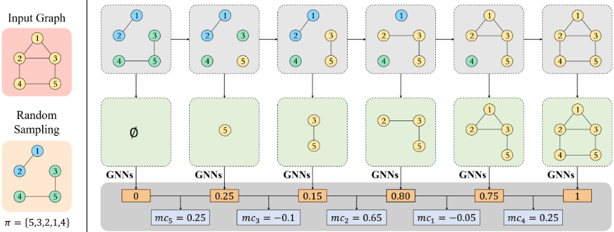
Most existing node-level explanation methods overlook the role of nodes in the graph structure and lack a solid theoretical foundation to evaluate the structural importance of nodes. We argue that the graph structure is a fundamental property of nodes, and explanations derived from structural features are more natural and theoretically grounded. To address this, we propose a method named GraphEXT, which models graph structure as an externality influencing GNN predictions and quantifies node importance through their interactions via the graph structure. Specifically, we introduce a graph-based game-theoretic framework incorporating Shapley value under externalities and adopt an efficient sampling strategy. The computed Shapley value serves as a quantitative measure of node importance, with the most significant nodes selected as the explanation result. Our approach is illustrated in Figure 1.
3.2 Externality of Graph Structure
As mentioned above, the quantification of node importance is based on the calculation of the Shapley value under externality defined in eq. (1). The relevant definitions of cooperative game theory will be extended to the graph domain in this section. Given the graph G = (X,A), let its node set be V = {v1, . . . , vn}, and define the set of players in the game as N = V . A subset of the node set, S = {vS1 , . . . , vSk }, forms a coalition. When only considering the nodes in the coalition S, the graph G is divided into several connected components, and the set of these connected components is defined as S | G:
Since the aggregation mechanism of GNN operates on each node and its neighboring nodes, the output of GNN for each connected component of the input graph is independent. Therefore, we havef (GS) = ∑
Here, GS represents the new graph (X,A ⊙ MSMST ) formed by removing all nodes in N \S and the edges incident to them from G.
Based on Myerson's definition [Myerson, 1977; Navarro, 2007], we define W(T,G) as the value function of a maximal connected component T in graph G, where its value is related to the internal structure of component T , meaning that the graph structure G exists as an externality. In this problem context, it is naturally assumed that W(T, G) = f(GT ). When the internal structure of GT changes, even if the set T remains the same, the value of W(T, G) must change accordingly. The above expression can be rewritten as:
Given the coalition structure P, the original graph is decomposed into a new graph GP based on the coalitions in P :
Based on the previous analysis, we can naturally define the value function of the current coalition game with the graph structure as an externality, V(S, P), as the output of GNN when the subgraph GS corresponding to coalition S is input under the structure GP :
The algorithm flow for this step is shown in Algorithm 1. First, we identify all edges whose endpoints belong to a same coalition in P and construct a subgraph of the original graph using these edges. The connected components of coalition S in the graph are found using a breadth-first search. Summing their corresponding outputs in the GNN gives the value of V(S, P). The computed value function V(S, P), together with the player set N, jointly defines the coalition game model we use.
To quantify the importance of each node, we adopt the Shapley value calculation method based on externality as proposed in Macho-Stadler's work[Macho-Stadler et al., 2007]:
where,
.
The advantage of this calculation method is that it does not require explicit modeling of externality (such as assuming a linear relationship or some specific form of externality), making it suitable for graph neural networks with blackbox properties. At the same time, it retains the efficiency, symmetry, and null-player properties of traditional Shapley values, ensuring fairness in the allocation algorithm theoretically. The computed Shapley values are directly used as the importance of each node. Since we use the GNN's prediction results as the value function for the coalition game when the graph structure changes, the physical meaning of the Shapley value leans more towards the contribution of nodes in the graph structure, offering a more fundamental explanation for the GNN's predictions.
3.3 Unbiased SamplingMethod
In practice, the exact calculation of the Shapley value requires considering all possible coalition structures. As the number
Algorithm 1 Compute the Network Based Value Function
Input: Model f(·), number of nodes n, graph G = (X,A),
- coalition S, coalition structure P Output: Value of V(S, P ) 1: for i = 1 to n do 2: outi ← {j | Aij = 1 and i, j belong to the same coalition } 3: end for 4: components ← [] 5: for i = 1 to n do 6: if i ∈ S and i has not been assigned to a connected component then 7: queue ← [i], visited ← {i} 8: while queue is not empty do 9: Extract the first element u 10: queue ← queue + (outu \ visited) 11: visited ← visited + outu 12: end while 13: components ← components + [visited] 14: end if 15: end for 16: return ∑R∈components f(GR)
of players increases, the computational complexity grows exponentially, so sampling methods are used to approximate the Shapley value.
As shown in eq. (1), when calculating the Shapley value for player i, there is a weight coefficient before the marginal contribution mc(S, i) for each coalition. It can be proven that:
Based on this result, when calculating the Shapley value for player i, we treat the weight coefficient as the probability of sampling the pair (π, P). In the m-th sampling step, we sample a pair (π, P) according to this probability and compute the marginal contribution mcm(i) for player i. Let the total number of sampling steps be T, and the average of the marginal contributions obtained from T samples is taken as the estimated Shapley value ˆ φi(V) for player i. Since the sampling steps are independent, it can be proven that this sampling method is unbiased:
Based on Skibski's work [Skibski et al., 2013], the weight function corresponding to the algorithm in eq. (2) is:
where P(i) represents the coalition in which player i is located in the coalition structure P. Referring to Skibski's
Algorithm 2 Shapley Value Sampling and Estimation
Input: Value function V(S, P), number of samples T Output: Shapley value for each player φz | z ∈ V
- 1: for all z ∈ v do φz ← 0 end for
- 2: for i = 1 to T do
- 3: π,A ← two random permutations generated using Knuth Shuffle
- 4: S ← ∅
- 5: Construct a directed graphwith n nodes and n directed edges based on permutation A, where the i-th edge points from node i to node A(i)
- 6: Identify all permutation cycles in the graph, with each cycle representing a coalition, and construct the initial partition P
- 7: for j = 1 to n do
- 8: Vbefore ← V(S, P )
- 9: S ← S ∪ {π(j)}, P → P[S]
- 10: Vafter ← V(S, P )
- 11: φπ(j) ←φπ(j) + 1 T (Vafter - Vbefore)
- 12: end for
- 13: end for
- 14: return φz | z ∈ V
work, to satisfy this weight function, we use the Kunth Shuffle to generate two random permutations, one of which is used as π, and the permutation cycles from the other are extracted. Each cycle is treated as a coalition to generate P .
In the algorithm implementation, we do not independently sample T permutations π for each player and construct the corresponding coalition C π i . Instead, at each sampling step, we sample a tuple (π, P) and iteratively move players out of their original coalitions into coalition S according to the order of the permutation π, with S initially being an empty coalition. It can be observed that after adding player π(i), the set S is equivalent to the coalition C π π(i) . This process continues until all players are added to S, and the marginal contribution of each player is computed for this sampling step. By averaging the marginal contributions over T samples, the Shapley value for each player is estimated. The specific algorithm for estimating Shapley values is shown in Algorithm 2.
3.4 Model Extensions
The above sections describes our proposed method using the graph classification task as an example. It is worth noting that this method can be adapted to explain node classification and link prediction models with appropriate adjustments. For node classification models, given a graph G, we aim to explain the model f(·)'s prediction for the target node vi. Since an L-layer graph neural network only considers the L-hop neighborhood of vi, we extract the L-hop subgraph centered on vi to reduce computational complexity. As the target of the model's prediction, vi must be included in every extracted connected component; otherwise, the model cannot classify vi. Based on this, we handle vi separately and modify the set of players in the coalition game model proposed in Section 3.2 to N \ {vi}. For a maximal connected component T formed by coalition S, if T ∪vi remains connected (i.e., there exists a node in T connected to vi), the value function is defined as W(T, G) = f(GT∪{vi}). Otherwise, W(T, G) = 0. When extracting the top-k important nodes as the explanation, we select the target node vi and the top k - 1 nodes ranked by Shapley value. For link prediction tasks, the goal is to explain the model's prediction for the existence probability of an edge (vi, vj). We extract the L-hop subgraph around vi and vj and treat the target node pair vi, vj separately. Correspondingly, we adjust the definitions of the characteristic function and the value function to adapt to this task.
4 Experimental Studies
4.1 Datasets and Baselines
We evaluated the effectiveness of GraphEXT using six datasets from node classification and graph-level classification tasks. The statistical details of these datasets are shown in Table 1. These datasets include synthetic datasets, sentiment graph datasets, and biological datasets.
BA-Shapes [Ying et al., 2019] is designed for node classification tasks, it is based on a Barab´asi-Albert graph with added house-like patterns. Nodes are categorized into four classes based on whether they are part of the house pattern and their positions within the pattern.
BA-2Motifs [Luo et al., 2020] is used for graph classification tasks, it is also based on a Barab´asi-Albert graph with two types of house-like patterns added. Graphs are classified into two categories based on the patterns.
Graph-SST2 and Graph-Twitter [Yuan et al., 2022] are used for graph classification tasks, these datasets transform textual data into graph representations, where nodes are words and edges are word associations. Each graph is classified based on its sentiment polarity (positive or negative).
BBBP and ClinTox [Wu et al., 2018] are designed for graph classification tasks, each graph in these datasets represents a molecule. Nodes are atoms, edges represent chemical bonds, and graph labels are determined by the molecule's chemical functions or properties.
| Datasets | Graphs | Nodes(avg) | Classes |
|---|---|---|---|
| BA-Shapes | 1 | 700 | 4 |
| BA-2Motifs | 1000 | 25 | 2 |
| BBBP | 2039 | 24.06 | 2 |
| ClinTox | 1478 | 26.16 | 2 |
| Graph-SST2 | 70042 | 10.20 | 2 |
| Graph-Twitter | 6940 | 21.10 | 2 |
In our experiments, we trained on all datasets using threelayer GCN [Kipf and Welling, 2016] and GIN [Xu et al., 2018] models. The model with the highest accuracy on the test set was selected as our final model, and all models were trained to achieve competitive accuracy. Subsequently, we chose several state-of-the-art methods for graph structure explanation as baselines, including FlowX [Gui et al., 2023], GNNExplainer [Ying et al., 2019], GradCAM [Pope et al., 2019], and PGExplainer [Luo et al., 2020]. The datasets and baseline implementations were based on the DIG Library [Liu et al., 2021].
4.2 Experimental Results on Datasets
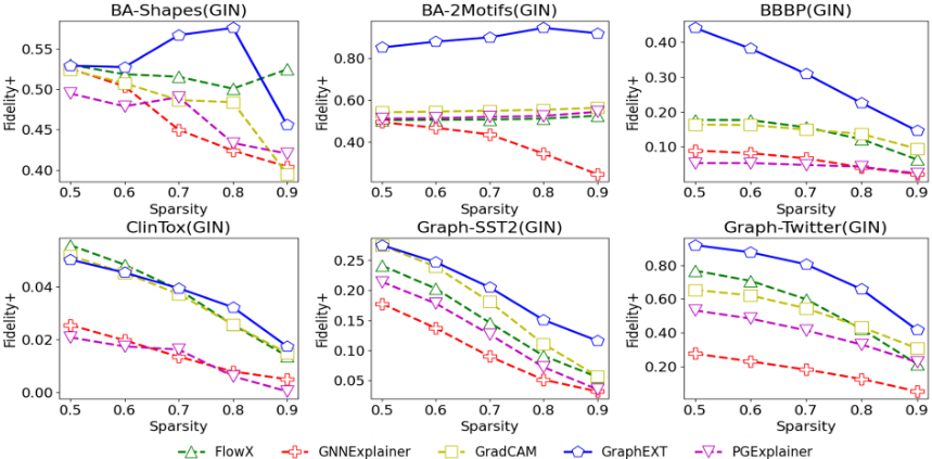
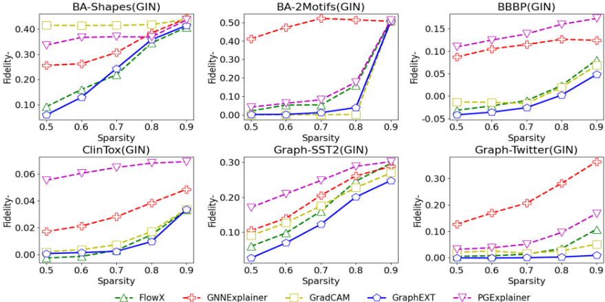
We adopted Fidelity+prob , Fidelity-prob [Yuan et al., 2021; Yuan et al., 2022], and Sparsity [Yuan et al., 2022] as evaluation metrics. Given a model f(·), a graph to be explained Gi = (Xi,Ai), the model's classification result yi, and the node mask Mi generated by the explanation method, these metrics are defined as follows:
Here, GM represents the new graph (X ⊙M,A) generated by retaining only the node features where M equals 1, mi = ∥M∥1 denotes the number of important nodes selected, and Mi indicates the total number of nodes in the graph. We evaluated our proposed GraphEXT on both synthetic and real-world datasets. For each dataset, we conducted quantitative calculations of the Fidelity metrics using test samples on trained GCN and GIN models to demonstrate the effectiveness of our method. The experimental results and analyses for the GIN model are presented in the main text. The results and related discussions for the GCN model are provided in the supplementary material for further reference.
We first conducted a quantitative analysis of Fidelity+ and Sparsity for different explanation methods. An ideal explanation method should accurately capture the critical features upon which the model's predictions are based. When these features are removed, the model's prediction probability should change significantly. Fidelity+ measures the probability change in the model's classification of the original input after removing the identified important features. A higher Fidelity+ score indicates that the method has identified more essential features. Sparsity evaluates the proportion of significant features to the total features in the original input, where a higher Sparsity score means fewer features are selected as critical. Ideally, a method should achieve higher Fidelity+ while maintaining lower Sparsity. Therefore, we compared the Fidelity+ scores of various methods under controlled Sparsity levels. As shown in Figure 2, our method outperforms baseline methods significantly at different Sparsity levels across most datasets. Even in datasets where it does not outperform, its performance is comparable to the best baseline methods.
Subsequently, we compared Fidelity- and Sparsity for different explanation methods. Fidelity- measures the probability change in the model's classification of the original input when only the important features are retained. Lower Fidelity- values indicate that the method can better preserve critical features. As shown in Figure 3, our method consistently achieves significantly lower Fidelity- than baseline methods in most datasets.
These experimental results demonstrate the robustness and generalization capabilities of our method across diverse datasets and model architectures. Furthermore, our method excels in explaining sentiment graph datasets, likely because such datasets often rely on a few sentiment-laden words to determine the overall sentiment. our method effectively quantifies the marginal contributions of these words within the graph structure, enabling more accurate explanations.
5 Conclusion
Graph Neural Networks (GNNs) are often regarded as black boxes, and improving their interpretability is a crucial research challenge. To address this issue, we propose GraphEXT, which introduces the concept of externality and integrates coalition game theory into the task of explaining GNNs. Our approach innovatively analyzes the impact of node transitions across different subgraphs on the model's predictions. Specifically, we leverage the Shapley value to quantitatively assess the importance of each node, delivering more interpretable results. Experimental findings demonstrate that GraphEXT consistently achieves superior interpretability across multiple synthetic and real-world datasets, as well as diverse GNN architectures. We believe this study not only offers a novel perspective for advancing GNN interpretability but also provides valuable insights for future research on graph-based modeling and explanation.
Acknowledgements
The authors gratefully acknowledge the reviewers for their valuable comments and suggestions. This research was supported by the National Natural Science Foundation of China (Grant No. 71601029) and the Sichuan Science and Technology Program (Grant No. 2025HJPJ0006). Lijun Wu is also supported by the student research project provided by the YingCai Honors College of the University of Electronic Science and Technology of China.
@inproceedings{ijcai2025p66,
  title     = {Explainable Graph Neural Networks via Structural Externalities},
  author    = {Wu, Lijun and Hao, Dong and Fan, Zhiyi},
  booktitle = {Proceedings of the Thirty-Fourth International Joint Conference on
               Artificial Intelligence, {IJCAI-25}},
  publisher = {International Joint Conferences on Artificial Intelligence Organization},
  editor    = {James Kwok},
  pages     = {583--591},
  year      = {2025},
  month     = {8},
  note      = {Main Track},
  doi       = {10.24963/ijcai.2025/66},
  url       = {https://doi.org/10.24963/ijcai.2025/66},
}
TY - CPAPER TI - Explainable Graph Neural Networks via Structural Externalities AU - Wu, Lijun AU - Hao, Dong AU - Fan, Zhiyi T2 - Proceedings of the Thirty-Fourth International Joint Conference on Artificial Intelligence, IJCAI-25 PB - International Joint Conferences on Artificial Intelligence Organization PY - 2025 SP - 583 EP - 591 DO - 10.24963/ijcai.2025/66 UR - https://doi.org/10.24963/ijcai.2025/66 ER -Copied
Machine-readable versions of this paper, for tools and AI agents:





