Explaining Black-box Model Predictions via Two-level Nested Feature Attributions with Consistency Property

1 Introduction

The rapid increase in size and complexity of machine learning (ML) models has led to a growing concern about their black-box nature. Models provided as cloud services are literal black boxes, as users have no access to the models themselves or the training data used. This opacity raises numerous concerns, including issues of trust, accountability, and transparency. Consequently, techniques for explaining the predictions made by such black-box models have been attracting significant attention [Danilevsky et al., 2020; Doˇsilovi´c et al., 2018; Saeed and Omlin, 2023].

∗The extended version of this paper, including detailed proofs and additional experimental results, is available at: https://arxiv.org/ abs/2405.14522.

Various model-agnostic local explanation methods have been proposed to explain the predictions of black-box models. Representative methods include, for example, local interpretable model-agnostic explanation (LIME) [Ribeiro et al., 2016] and kernel Shapley additive explanations (Kernel SHAP) [Lundberg and Lee, 2017], which estimate the feature attributions for the individual prediction by approximating the model's behavior with local linear surrogate models around the input.

In LIME and Kernel SHAP, the input to the model is generally assumed to be a flat structure, where the input features are treated as independent variables. In many realistic tasks for various domains, such as image, text, geographic, e-commerce, and social network data, however, the input features have a nested structure that consists of high- and lowlevel features, and each high-level feature is decomposed into multiple low-level features. A typical task with such nested features is multiple instance learning (MIL) [Ilse et al., 2018] where the model is formulated as a set function [Kimura et al., 2024]. In MIL, the input is a set of instances, the highlevel feature is an instance in the set, and the low-level features represent the features of the instance. In addition, even if the input is not represented in a nested structure when it is fed into the model, it may be more natural to interpret it with the nested structure. For example, although a text input is usually represented as a sequence of words, it is natural to interpret it as having high-level features such as phrases, sentences, and paragraphs.

The two-level features enable us to understand the model predictions with two types of feature attributions at different levels of granularity, which we name high-level feature attributions (HiFAs) and low-level feature attributions (LoFAs), respectively. Figure 1 shows an example of the prediction for a nested-structured input and its corresponding HiFAs and LoFAs. The HiFAs represent how much each of the high-level features contributes to the prediction. These are also referred to as instance attributions in the MIL literature [Early et al., 2022; Javed et al., 2022], which are used to reveal which instances strongly affected the model's decision. On the other hand, the LoFAs represent how much each of the low-level features contributes to the prediction, providing a finer-grained explanation of how the components of the instances affected the prediction. Both the HiFAs and LoFAs are important for understanding the model's decision. However, existing studies have focused on estimating either-level attributions, and no study has addressed estimating the HiFAs and LoFAs simultaneously.

For the estimation of the HiFAs and LoFAs, two naive approaches can be applied. One is to estimate the HiFAs and LoFAs separately by applying existing model-agnostic local explanation methods to the high- and low-level features, respectively. The other is to estimate the LoFAs first, as in the former approach, and then estimate the HiFAs by aggregating the LoFAs. However, these approaches have two limitations in terms of leveraging the nested structure of the input. First, even though the queries to the black-box model are often limited in practice due to the computational time and request costs, the input structure is not utilized to reduce the number of queries in the estimation. Second, the former approach can produce mutually inconsistent HiFAs and LoFAs. For example, the high-level feature identified as most influential (highest HiFA) might not coincide with the high-level feature that contains the most influential low-level feature (highest LoFA).

To address these issues, we propose a model-agnostic local explanation method that effectively exploits the nested structure of the input to estimate the HiFAs and LoFAs simultaneously. A key idea of the proposed method is to introduce the consistency property that should exist between the HiFAs and LoFAs, thereby bridging the separate optimization problems for them. We solve a joint optimization problem to estimate the HiFAs and LoFAs simultaneously with the consistency constraints depicted in Figure 1 based on the alternating direction method of multipliers (ADMM) [Boyd et al., 2011]. The algorithm is a general framework that can also introduce various types of regularizations and constraints for the HiFAs and LoFAs, such as the ℓ1 and ℓ2 regularizations and nonnegative constraints, which lead to the ease of interpretability for humans.

In experiments, we quantitatively and qualitatively assess the HiFAs and LoFAs estimated by the proposed method on image classification in the MIL setting and text classification using language models. The experimental results show that the HiFAs and LoFAs estimated by the proposed method 1) satisfy the consistency property, 2) are faithful explanations to the black-box models even when the number of queries to the model is small, 3) can accurately guess the ground-truth positive instances and their features in the MIL task, and 4) are reasonable explanations visually.

The contributions of this work are summarized as follows:

• This study is the first to propose a model-agnostic local explanation method to estimate the two-level nested feature attributions simultaneously, which satisfies the consistency property between them.
• To justify the behavior of the proposed method, we provide theoretical analysis in terms of the existence and uniqueness of the solution and the convergence of the optimization algorithm.
• In the experiments on practical tasks, we demonstrate that the proposed method can produce accurate, faithful,

and consistent two-level feature attributions with a smaller number of queries to the black-box models.

2 RelatedWork

Numerous methods for explaining the individual predictions of black-box models have been proposed in the literature [Ribeiro et al., 2016; Lundberg and Lee, 2017; Ribeiro et al., 2018; Petsiuk et al., 2018; Plumb et al., 2018]. A versatile approach is to explain feature attributions estimated by approximating the model predictions with surrogate models around the input, such as LIME [Ribeiro et al., 2016] and Kernel SHAP [Lundberg and Lee, 2017]. The proposed method is in line with this type of approach.

One example of a nested input structure is set data, where a set of multiple instances is treated as a single input. Set data appears in various ML applications, such as point cloud classification [Guo et al., 2021], medical image analysis [Cheplygina et al., 2019], and group recommendation [Dara et al., 2020], and the explainability in those applications has also been studied in the literature [Tan and Kotthaus, 2022; van der Velden et al., 2022]. Unlike our work, most such studies focus only on estimating instance attributions corresponding to those of high-level features. For example, Early et al. proposed to estimate instance attributions by learning surrogate models with MIL-suitable kernel functions [Early et al., 2022].

Several studies have addressed estimating feature attributions effectively by leveraging group information of input features. In the natural language processing literature, some studies estimated sentence- and phrase-level feature attributions by grouping words in the same sentence and phrase together and regarding them as a single feature [Zafar et al., 2021; Mosca et al., 2022]. In addition, Rychener et al. showed that word-level feature attributions can be improved by generating perturbations at a sentence level, mitigating out-of-distribution issues for the model and the challenges of a high-dimensional search space [Rychener et al., 2023]. In the official SHAP library [shap (GitHub), 2024], by grouping input features by hierarchical clustering in advance and generating perturbations at the group level, one can reduce the number of queries to the model.

3 ProposedMethod

3.1 Two-level Nested Feature Attributions with Surrogate Models

The model f to be explained is a trained black-box model that takes an arbitrary input, such as tabular, image or text, x ∈ X, and outputs a prediction y = f(x) ∈ [0, 1]C where X is the input space, and C is the number of classes. The input x consists of two-level nested features, referred to as high-level and low-level features, with each high-level feature being decomposed into multiple low-level features. In particular, the input x is represented as a set or sequence of J high-level features, i.e., x = {xj}Jj=1 where xj ∈ RDj is a Dj-dimensional low-level feature vector representing the j-th high-level feature. One example of such input appears in image classification under the MIL setting. In this setting, the input is a bag of images, the high-level feature is an image in the bag, and the low-level features correspond to super-pixels in the image. Another example appears in a document classification where the input is a sequence of sentences, the highlevel feature is a sentence in the sequence, and the low-level features correspond to the words in the sentence.

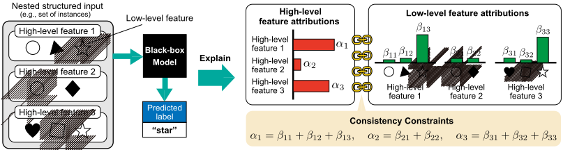
We consider estimating the high-level feature attributions (HiFAs) and low-level feature attributions (LoFAs) that explain the prediction of the black-box model f for the input x using surrogate models as with LIME and Kernel SHAP. The HiFAs and LoFAs represent how much the high- and low-level features in the input contribute to the prediction, respectively. In the aforementioned MIL setting, the HiFAs represent how much images in the input bag contribute to the prediction, which is also referred to as instance attributions in the literature, and the LoFAs represent how much the super-pixels in the images contribute to the prediction. To estimate the HiFAs and LoFAs, we introduce two-level local linear surrogate models for high-level and low-level features, eH and eL , that mimic the behaviors of the black-box model f around the input x, as follows:

(1) where zH ∈ {0, 1}J and zL = {zL j }Jj=1 with zL j ∈ {0, 1}Dj are simplified inputs associated with the input x, which are used to indicate the presence or absence of the high- and lowlevel features in x, respectively; α ∈ RJ and β = {βj}Jj=1 with βj ∈ RDj are the learnable coefficients of these surrogate models, and after learning, they will be the HiFAs and LoFAs themselves, respectively. For ease of computation, we define the concatenation of β and zL over the highlevel features as β† = concat(β1, β2, · · · , βJ) ∈ RD† and zL† = concat(zL 1 , zL 2 , · · · , zL J ) ∈ {0, 1}D† , where D† = ∑Jj=1 Dj .

The surrogate models are learned with the predictions of the black-box model f for perturbations around the input x. The perturbations are generated by sampling the simplified inputs zH and zL† from binary uniform distributions and then constructing masked inputs ϕHx (zH), ϕLx(zL† ) ∈ X depending on the simplified inputs, respectively. Here, ϕHx and ϕLx are mask functions that replace the input x's dimensions associated with the dimensions being zero in the simplified inputs zH and zL† with uninformative values, such as zero, respectively. Let ZH ∈ {0, 1}NH×J and ZL ∈ {0, 1}NL×D† be the matrices whose rows are the generated simplified inputs for the high- and low-level features, respectively, where NH and NL are the numbers of perturbations used to estimate the HiFAs and LoFAs, respectively. Also, let ˜ yH = [˜ yH 1 , ˜ yH 2 , · · · , ˜ yHNH ]⊤ ∈ RNH×C and ˜ yL = [˜ yL 1 , ˜ yL 2 , · · · , ˜ yLNL ]⊤ ∈ RNL×C be the predictions of the black-box model for the perturbations where ˜ yH n = f(ϕHx (ZH n )) and ˜ yL n = f(ϕLx(ZL n )).

The parameters of the surrogate models, i.e., the HiFAs ˆα and LoFAs ˆ β† , can be estimated by solving the following weighted least squares separately:

where W H ∈ RNH×NH and W L ∈ RNL×NL are the diagonal matrices whose nth diagonal elements represent the sample weights for the nth perturbation; ΩH and ΩL are the regularizers for the HiFAs and LoFAs, respectively; λH ≥ 0 and λL ≥ 0 are the regularization strengths.

3.2 Optimization with Consistency Constraints

Although the HiFAs and LoFAs provide different levels of explanations, these explanations for the same black-box model should be consistent with each other. Owing to the linearity of the surrogate models and the fact that each high-level feature can be decomposed into low-level features, the following property is expected to hold:

Property 1 (Consistency between two-level feature attributions).

In other words, the HiFA for each high-level feature is equal to the sum of the LoFAs of its constituent low-level features.

The two surrogate models defined in (1) that satisfy the consistency property behave equivalently for simplified inputs zH and zL under the condition if zH j = 0 then zL j = 0Dj , and if zH j = 1 then zL j = 1Dj where 0Dj and 1Dj are the Dj-dimensional zero and one vectors, respectively.

The consistency property is essential for providing consistent and convincing explanations to humans. However, in practice, it is often not satisfied for two reasons. First, the number of perturbations may be insufficient to accurately estimate the feature attributions because the number of queries to the model f is often limited due to computational time and request costs. Second, in the predictions for the perturbations, the model f's behavior can differ depending on whether the high-level features or the low-level features are masked out because of missingness bias [Jain et al., 2022]. To overcome these problems, the proposed method estimates the HiFAs and LoFAs simultaneously by solving the following optimization with consistency constraints:

The consistency constraints bridge the gap between the two surrogate models, forcing them to behave equivalently. This helps compensate the insufficiency of the queries to the model and mitigate the negative effects of the missingness bias on the estimation of the HiFAs and LoFAs.

We solve the optimization problem based on the alternating direction method of multipliers (ADMM) [Boyd et al., 2011]. The detailed derivation of the optimization algorithm is provided in Appendix A. An advantage of employing the ADMM is that, despite the interdependence of α and β† caused by the consistency constraints, they can be estimated independently as in (2) and (3). In addition, the solution has another advantage: it allows the inclusion of various types of regularizations and constraints for α and β, such as sparsity regularization and non-negative constraints in ΩH and ΩL. The optimization algorithm is provided in Algorithm 1 in Appendix A.

4 Auxiliary Theoretical Analysis

In this section, we provide theoretical analysis for the proposed method, referred to as Consistent Two-level Feature Attribution (C2FA), to justify its behavior. See Appendix C for proof sketches of all statements in this section. In this section, we impose the following assumptions.

Assumption 4.1 (Convexity). LH(·), LL(·), ΩH(·), ΩL(·) are convex in their respective parameters. Specifically, each loss term is weighted least squares loss, and each regularizer is a convex function.

Assumption 4.2 (Strict Feasibility). There exists (α◦ , β◦ ) such that α◦ j = ∑Dj d=1 β◦ j,d for all j, ensuring the constraint set is non-empty.

Assumption 4.3 (Non-degeneracy). The design matrices underlying zH and zL have full column rank in typical regression settings. This ensures identifiability of α and β.

Assumption 4.4 (Bounded Outputs). Black-box outputs {f(xi)}Ni=1 lie in a bounded set, or at least have finite second moments, ensuring the objective is well-defined and finite.

Assumption 4.5 (Parameter Domains). α and β lie in closed, convex domains Γα and Γβ.

Define the feasible set

and define J(α, β) := LH(α) + LL(β) + λHΩH(α) + λLΩL(β). Hence the optimization problem is min(α,β)∈Γ◦ J (α, β). We develop existence and uniqueness of solutions under mild conditions, as well as the precise satisfaction of αj = ∑Dj d=1 βj,d at optimality. We first establish that a global minimizer exists. Under additional strict convexity conditions, we also show uniqueness

Lemma 4.6 (Existence of a Global Minimizer). Under assumptions, there exists at least one global minimizer (α∗ , β∗ ) of C2FA optimization.

Lemma 4.7 (Strong Convexity and Uniqueness). Suppose that the high-level and low-level losses LH and LL are strictly convex quadratic forms in α and β, respectively (e.g., weighted least-squares with full column rank), and ΩH,ΩL are either strictly convex or affine so as not to destroy strict convexity of the overall objective. Then any global minimizer (α∗ , β∗ ) is unique.

Theorem 4.8. Let ˜α be an unconstrained minimizer of LH(α) + λHΩH(α), and let ˜α be an unconstrained minimizer of LL(β) + λLΩL(β). Then, if ( ˜α, ˜ β) do not already satisfy ˜αj = ∑d ˜ βj,d for each j, any global minimizer (α∗ , β∗ ) of the C2FA optimization achieves strictly smaller objective value: J (α∗ , β∗ ) < J ( ˜α, ˜ β).

Next, we provide the convergence analysis based on the concentration inequality.

Theorem 4.9 (High-Probability Convergence of C2FA). Let {(zHn , Y H n )}NH n=1 and {(zLn , Y L n )}NL n=1 be i.i.d. samples drawn from some distribution of mask vectors (for high-level and low-level features) and black-box outputs, with sub-Gaussian or bounded noise. Form the matrices ZH ∈ RNH×J and ZL ∈ RNL×D† by stacking zHn , zLn , and similarly stack Y H, Y L . Suppose the following:

• (i) The random design satisfies a restricted eigenvalue property on ZH and ZL with high probability.
• (ii) The losses LH and LL are given by weighted least squares, and the regularizers ΩH, ΩL are convex.
• (iii) αj = ∑Dj d=1 βjd for each j = 1, . . . , J.
• (iv) Let (α⋆ , β⋆ ) be the minimizer of the expected version of the same objective under that constraint, i.e. the best consistent linear approximation of f in expectation.

Then, for any δ ∈ (0, 1), with probability at least 1 - δ, the solution (̂α, ̂ β) to the finite-sample C2FA problem satisfies

where C > 0 is a constant depending on sub-Gaussian parameters, the restricted eigenvalue lower bound, and the regularization strengths.

Corollary 4.10 (Uniform Approximation Guarantee). Assume the same setting as Theorem 4.9 and let eH(zH) = (zH)⊤ ̂α and eL (zL ) = (zL )⊤ ̂ β be the final C2FA surrogate models. Further suppose that zH and zL take values in some bounded set Z H ⊆ RJ and Z L ⊆ RD† respectively. Then with probability at least 1 - δ,

for some constant ˜ C,BH, ϵ∗ depending on sub-Gaussian parameters, bounding sets Z H,Z L , and the regularization strengths.

5 Experiments

We conducted experiments on two tasks of image and text domains to evaluate the effectiveness of the proposed method, referred to as C2FA, implemented with Algorithm 1 in Appendix A. Its hyperparameters are provided in Appendix B.

Comparing Methods. We used five methods for comparison: LIME [Ribeiro et al., 2016], MILLI [Early et al., 2022], Bottom-Up LIME (BU-LIME), Top-Down LIME (TDLIME), and Top-Down MILLI (TD-MILLI). With LIME, we estimated the HiFAs and LoFAs separately by solving (2) and (3), respectively, where we used the cosine kernel for the sample weights and ℓ2 regularization for ΩH and ΩL. MILLI is the state-of-the-art instance attribution method in the MIL setting, which was proposed for estimating only the HiFAs. Therefore, we estimated the LoFAs in MILLI in the same way as in LIME. With BU-LIME, we first estimated the LoFAs using LIME and then calculated the HiFAs of each high-level feature by summing the LoFAs associated with the high-level feature. This method always satisfies the consistency property because the HiFAs are calculated from the LoFAs. With TD-LIME and TD-MILLI, we first estimated the HiFAs using LIME and MILLI, respectively. Then, for the jth high-level feature, we determined its LoFAs βj by sampling from a normal distribution with mean αj (the jth HiFA) and the standard deviation 1/Dj . Finally, we enforced the consistency property by adjusting one randomly selected low-level feature for each high-level feature j: we set that feature's LoFA to βjd = αj - ∑d′∈[Dj]\{d} βjd′ , ensuring that ∑d′∈[Dj ] βjd′ = αj .

5.1 Multiple Instance Image Classification

Dataset. We constructed an MIL dataset from the Pascal VOC semantic segmentation dataset [Everingham et al.,

2015] with the ground-truth instance- and pixel-level labels. Each sample (bag) contains three to five images, randomly selected from the Pascal VOC dataset. Here, low-level features correspond to regions (super-pixels) of each image. Each bag is labeled positive if at least one image in the bag is associated with the "cat" label; otherwise the bag is negative. Also, each image pixel is labeled positive if it is associated with the "cat" label, and negative otherwise. A detailed description of the dataset is provided in Appendix B.

Black-box Model. We used a DeepSets permutationinvariant model [Zaheer et al., 2017] with ResNet-50 [He et al., 2016] as the black-box model f to be explained. We describe the implementation details of the model in Appendix B. Here, the test accuracy of the model was 0.945.

Quantitative Evaluation. We assessed the estimated HiFAs and LoFAs in terms of correctness, faithfulness, and consistency. Correctness is evaluated using the ground-truth instance- and pixel-level labels. Following the evaluation in the MIL study [Early et al., 2022], we evaluated the estimated HiFAs with normalized discounted cumulative gain (NDCG). Additionally, by regarding the estimated LoFAs as the predictions of the pixel-level labels, we evaluated them with the area under ROC curve (AUROC) in a binary semantic segmentation setting. In the faithfulness evaluation, we assessed whether the estimated HiFAs and LoFAs are faithful to the behaviors of the model f based on insertion and deletion metrics [Petsiuk et al., 2018]. For consistency, we used the following two metrics. The first one is the consistency between the estimated HiFAs and LoFAs, measured by ∥α-Mβ† ∥2 , which is the same quantity used as the consistency penalty in (7). The second one is the agreement of the most important high- and low-level feature (MIHL). We ran the evaluations three times with different random seeds and reported the average scores and their standard deviations. The details of the evaluation metrics are provided in Appendix B.

Results. Figure 2a shows the NDCG and deletion scores of the estimated HiFAs over various numbers of perturbations for the LoFAs, NL, where we fixed the number of perturbations for the HiFAs, NH = 5. We found that the proposed method (C2FA) consistently achieved the best NDCG and deletion scores, and the superiority of the proposed method is especially noticeable when NL is small. Although BULIME improved the scores as NL increased, the scores were still lower than those of the proposed method. Since the other comparing methods estimate the HiFAs without the effects of the LoFAs, their scores were constant regardless of the value of NL.

Figure 2b shows the AUROC and deletion scores of the estimated LoFAs over various values of NL where we fixed NH = 20. When NL is small, we found that the proposed method achieved significantly better AUROC and deletion scores. In particular, the AUROC score of the proposed method at NL = 50 was comparable to that of the secondbest methods, LIME, MILLI, and BU-LIME, at NL = 150, and the deletion score of the proposed method at NL = 50 was much the same as that of the second-best methods at NL = 100. These results show that the proposed method is very efficient in terms of the number of queries to the model Input (bag of images)

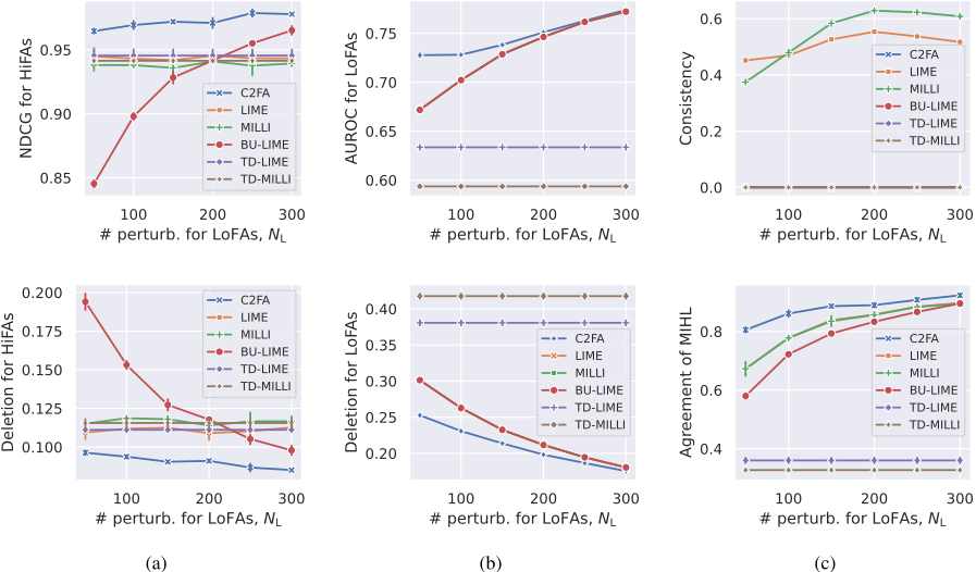
f, thanks to the simultaneous estimation of the HiFAs and LoFAs.

Figure 2c shows the consistency scores and the agreement scores of MIHL over various values of NL where we fixed NH = 20. Here, the consistency scores of BU-LIME, TDLIME, and TD-MILLI are always zero by definition. We found that the consistency scores of LIME and MILLI were worse because they estimated the HiFAs and LoFAs separately. On the other hand, those of the proposed method were nearly zero, which means that the estimated HiFAs and LoFAs satisfied the consistency property. With the agreement scores of MIHL, we found that the proposed method outperformed the other methods regardless of the values of NL, and the differences in the scores were especially noticeable for smaller NL values (i.e., NL ≤ 150).

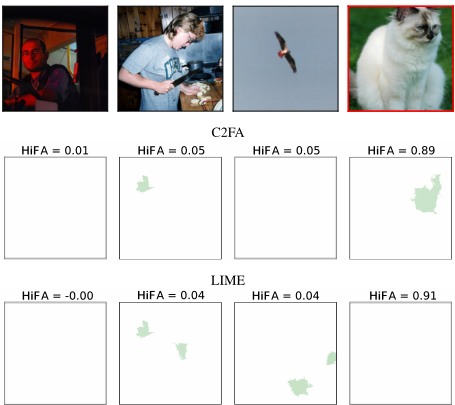
We visualize an example of the estimated HiFAs and LoFAs by the proposed method and the best-performing baseline, LIME, in Figure 3. Here, we only display the LoFAs larger than 0.1 for clarity. The figure shows that the proposed method assigned a high LoFA to the super-pixel in the high-level feature which was the positive instance and had the highest HiFA (HiFA = 0.89), although LIME assigned high LoFAs to the super-pixels in the negative instances. The critical difference between the two methods is whether the HiFAs and LoFAs are estimated simultaneously or separately. Since both the proposed method and LIME assigned the highest HiFA to the positive instance correctly, the result indicates that estimating the HiFAs and LoFAs simultaneously is effective.

5.2 Text Classification Using Language Models

Another practical application of the proposed method is to explain the attributions of sentences and the words in text classification with language models.

Dataset. We constructed a dataset in which the validation and test sets contain 500 and 1,000 product reviews, respectively, randomly sampled from the Amazon reviews dataset [Zhang et al., 2015], respectively. Each sample consists of multiple sentences (high-level features), where each sentence is a sequence of words (low-level features). The label of each sample corresponds to the review's sentiment polarity (positive or negative).

Black-box Model. We used BERT [Devlin et al., 2018] fine-tuned on the original Amazon reviews dataset, which is provided on Hugging Face [fabriceyhc (Hugging Face), 2022]. The test accuracy of the model is 0.947. When masking a word in the input to generate perturbed inputs, we replaced the word with the predefined mask token [MASK]. Similarly, when masking a sentence, we replaced all the words in the sentence with the mask token.

Quantitative Evaluation. Because no ground-truth labels for HiFAs and LoFAs are available in the dataset, we evaluated the estimated HiFAs and LoFAs only in terms of faithfulness and consistency, as in Section 5.1.

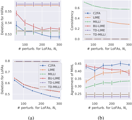
Results. Figure 4a shows the deletion scores of the estimated HiFAs and LoFAs over various values of NL where we fixed NH = 5 and 50, respectively. With the deletion scores of the HiFAs, although the scores of the proposed method were equal to or worse than those of MILLI and TD-MILLI at NL ≤ 150, the proposed method achieved the best deletion score at NL ≥ 200. We found that in this task, the LIMEbased methods, including the proposed method, were worse than the MILLI-based methods at small NL values. As NL increased, the proposed method benefited from the consistency constraints and became the only LIME-based method that outperformed the MILLI-based methods. With the deletion scores of the LoFAs, the proposed method outperformed the other methods regardless of the values of NL.

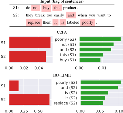
Figure 4b shows the consistency scores and the agreement scores of MIHL over various values of NL where we fixed NH = 50. Again, in this task, the consistency scores of the proposed method were nearly zero regardless of the values of NL. With the agreement scores of MIHL, the proposed method maintained high scores regardless of the values of NL, although the scores of BU-LIME were slightly better than the proposed method at NL ≤ 100.

Figure 5 shows an example of the HiFAs and LoFAs estimated by the proposed method and the second-best method, BU-LIME. In the example, we fixed NH = 50 and NL = 50; that is, NL is insufficient to estimate the LoFAs accurately. We found that although the baseline method assigned higher LoFAs to the words in the second sentence (S2), the proposed method assigned higher LoFAs to the words in the first sentence (S1). This is because the proposed method regularizes the LoFAs via the consistency constraints, exploiting the fact that S1 has a high HiFA.

6 Conclusion

We hypothesized that the consistency property, which is naturally derived from the characteristics of surrogate models, is essential for producing explanations that are accurate, faithful, and consistent between HiFAs and LoFAs. This property also enables the method to require fewer queries to the model.

To address this, we proposed a model-agnostic local explanation method for nested-structured inputs, that is capable of explaining two-level feature attributions. Our experiments on image and text classification tasks demonstrated that the proposed method can efficiently generate high-quality explanations while using fewer queries. Future work includes extending the method to handle more complex nested structures and exploring additional application domains.

A Optimization Algorithm

Our objective to estimate the HiFAs and LoFAs simultaneously is as follows:

We solve the optimization based on the alternating direction method of multipliers (ADMM) [Boyd et al., 2011]. By introducing auxiliary variables ¯α ∈ RJ and ¯ β† ∈ RD† and Lagrange multipliers v1 ∈ RJ , v2 ∈ RD† , and v3 ∈ RJ based on the ADMM manner, our objective is rewritten as follows:

where h1(α, ¯α) = α - ¯α, h2(β† , ¯ β† ) = β† - ¯ β† , h3(α, β† ) = α-Mβ† . Here, M ∈ {0, 1}J×D† is a binary matrix to add up the LoFAs associated with the same highlevel feature where we set to Mjd = 1 if the dth feature of the concatenated input x† belongs to the jth high-level feature xj, and Mjd = 0 otherwise. The hyperparameters µ1 ≥ 0 and µ2 ≥ 0 are the penalty parameters for the regularization and the consistency constraint, respectively.

The optimization of (7) is performed by alternating the updates of the variables iteratively. We summarize the optimization algorithm using ℓ2 regularization for ΩH and ΩL in Algorithm 1. Here, IJ and ID† are identity matrices of size J and D† , respectively, and in Line 9, the variables at the zeroth step are initialized with zero. The algorithm is terminated when ∥ ¯αt-1 - ¯αt ∥2 + ∥ ¯ β†t-1 - ¯ β†t ∥2 < ϵ1 and ∥h1(αt , ¯αt )∥2 + ∥h2(β†t , ¯ β†t )∥2 + ∥h3(αt , β†t )∥2 < ϵ2 where ϵ1, ϵ2 ≥ 0 are hyperparameters. The other hyperparameters of the algorithm are λH, λL, µ1, and µ2.

B Experiments on Image Classification in Multiple Instance Learning

Detailed Description of Dataset. We constructed an MIL dataset from the Pascal VOC semantic segmentation Algorithm 1 Estimating consistent two-level feature attributions (C2FA) with ℓ2 regularization

• 1: Generate binary random matrices ZH and ZL
• 2: Obtain perturbed inputs { ˜XH n }NH n=1 and { ˜XL n }NL n=1 using ϕH and ϕL
• 3: Obtain predictions ˜ yH and ˜ yL from the perturbed inputs
• 4: Obtain weight matrices W H and W L

dataset [Everingham et al., 2015] that allows us to evaluate the estimated HiFAs and LoFAs with the ground-truth instance- and pixel-level labels. With the training subset of the dataset, each bag contains **three to five images**, randomly selected from the Pascal VOC dataset. Here, low-level features correspond to regions (super-pixels) of each image, which are obtained by the quick shift algorithm [Vedaldi and Soatto, 2008]. Each bag is labeled positive if at least one image in the bag is associated with the "cat" label; otherwise the bag if negative. Also, each image pixel is labeled positive if the pixel is associated with "cat" label and negative otherwise. We used the instance- and pixel-level supervision only for evaluation. Similarly, we constructed validation and test subsets whose samples contain images from the training and test subsets of the Pascal VOC, respectively. The number of samples in training, validation, and test subsets is 5,000, 1,000, and 2,000, respectively, and the positive and negative samples ratio is equal.

DetailedDescription of Dataset. We defined the DeepSets permutation-invariant model [Zaheer et al., 2017] as a blackbox model f to be explained. According to [Zaheer et al., 2017], the model f comprises two components: a representation function that transforms each instance, ϕ, and a nonlinear network that produces predictions from the extracted representation, ρ. We used ResNet-50 [He et al., 2016] pretrained on ImageNet as the representation function ϕ and twolayer multi-layer perceptron (MLP) as the non-linear network ρ. Here, in ρ, we used the ReLU activation function for the first layer and the softmax function for the second layer. Also, the number of hidden units in the MLP was set to 1,024. The model first extracts the representation of each instance using ϕ, then adds them up into a single representation, and finally, outputs a prediction by applying ρ to the aggregated single representation. We trained the model using our MIL image classification dataset with Adam optimizer [Kingma and Ba, 2015] with a learning rate of 0.001, a batch size of 32, and a maximum epoch of 300. The test accuracy of the model was 0.945.

The hyperparameters of C2FA, λH, λL, and µ1, were tuned using the validation subset of each dataset within the following ranges: λH, λL ∈ {0.1, 1}, and µ2 ∈ {0.001, 0.01, 0.1}. The remaining hyperparameters were set to µ1 = 0.1 and ϵ1 = ϵ2 = 10-4 . The experiments were conducted on a server with an Intel Xeon Gold 6148 CPU and an NVIDIA Tesla V100 GPU.

Detailed Description of Quantitative Evaluation Metrics. We assessed the estimated HiFAs and LoFAs in terms of correctness, faithfulness, and consistency. The correctness is evaluated using the ground-truth instance- and pixel-level labels. Following the evaluation in the MIL study [Early et al., 2022], we evaluated the estimated HiFAs using normalized discounted cumulative gain (NDCG). For the estimated LoFAs, as with the evaluation of the LoFAs for single image classification [Sampaio and Cordeiro, 2023], we evaluated them as the predictions of the pixel-level labels by the area under ROC curve (AUROC) in the binary semantic segmentation manner. For faithfulness, we assessed whether the estimated HiFAs and LoFAs are faithful to the behaviors of the model f using insertion and deletion metrics [Petsiuk et al., 2018]. The insertion and deletion metrics evaluate the change in the predictions of the model f when features deemed important in the LoFAs are gradually added and removed from the sample, respectively. In our experiments, we gradually add and remove the low-level features across all the highlevel features in descending order of their LoFAs. Also, for the HiFAs, we add and remove the high-level features instead of the low-level ones, respectively. In terms of the consistency evaluation, we used the following two metrics. The first one is the consistency between the estimated HiFAs and LoFAs, which is calculated with ∥α-Mβ† ∥2 used to calculate the penalty for the consistency constraints in (7). The second one is the agreement of the most important high- and lowlevel feature (MIHL), which is calculated by the ratio that the high-level feature of the highest HiFA is identical to the one associated with the low-level feature of the highest LoFA.

We evaluated the above metrics using only the samples with the positive bag label because we could not evaluate the correctness of those with the negative bag label. We ran the evaluations three times with different random seeds and reported the average scores and their standard deviation.

C Proof Sketches

Sketch of Proof for Lemma 4.6. By assumptions, the loss functions LH(·), LL(·), as well as the regularizers ΩH(·), ΩL(·) are convex in their respective parameters. Since the objective function J is convex, lower bounded, and the feasible set Γ◦ is non-empty, closed and convex, by the Weierstrass extreme value theorem, there exists at least one global

minimizer (α∗ , β∗ ) ∈ Γ◦ .

Sketch of Proof for Lemma 4.7. Under Assumption 4.3 each quadratic loss is strictly convex. Adding any convex regulariser keeps strict convexity. The sum of two strictly convex functions on a linear subspace is strictly convex, so the constrained optimisation has a single global minimiser.

Sketch of Proof for Theorem 4.8. Let ˜αand ˜ β be the separate ridge/LIME minimisers. By assumption they violate at least one consistency equation. Project them onto Γ◦ by defining α◦j := ∑d ˜ βjd, β◦ := ˜ β. Owing to strict convexity, the affine projection strictly decreases the joint objective unless the constraint already held. The global constrained minimiser therefore attains strictly lower objective value than the naive concatenation (α◦ , β◦ ).

Sketch of Proof for Theorem 4.9. Treat the joint parameter vector θ = (α, β) ∈ RJ+D† , lying in a linear subspace of rank J + D† - J. With sub-Gaussian masks, empirical Gram matrices for both high- and low-level designs satisfy a restricted-eigenvalue (RE) bound with probability 1 - δ as λmin(ˆΣ). Standard stochastic-convex-optimisation argument gives excess-risk and constant C absorbs RE constant, variance proxy, and regularization strengths.

Sketch of Proof for Corollary 4.10. Split the pointwise approximation error into (population) linear-model bias plus parameter-estimation error, and under bounded design ∥zH ∥ ≤ BH the first term is bounded by BH∥̂α - α∗ ∥2. Insert the rate from Theorem 4.8 and add the analogous lowlevel term, yielding the stated uniform bound with probability 1 - δ.

Acknowledgments

This work was supported by JSPS KAKENHI Grant Number 22K17953.