
Dual-Balancing for Physics-Informed Neural Networks
Proceedings of the Thirty-Fourth International Joint Conference on Artificial Intelligence. Main Track. Pages 7164-7172.
https://doi.org/10.24963/ijcai.2025/797
Keywords
- Machine Learning: ML: Optimization
- Machine Learning: ML: Applications
- Machine Learning: ML: Regression
- Multidisciplinary Topics and Applications: MTA: Physical sciences
Abstract
Physics-informed neural networks (PINNs) have emerged as a new learning paradigm for solving partial differential equations (PDEs) by enforcing the constraints of physical equations, boundary conditions (BCs), and initial conditions (ICs) into the loss function. Despite their successes, vanilla PINNs still suffer from poor accuracy and slow convergence due to the intractable multi-objective optimization issue. In this paper, we propose a novel Dual-Balanced PINN (DB-PINN), which dynamically adjusts loss weights by integrating inter-balancing and intra-balancing to alleviate two imbalance issues in PINNs. Inter-balancing aims to mitigate the gradient imbalance between PDE residual loss and condition-fitting losses by determining an aggregated weight that offsets their gradient distribution discrepancies. Intra-balancing acts on condition-fitting losses to tackle the imbalance in fitting difficulty across diverse conditions. By evaluating the fitting difficulty based on the loss records, intra-balancing can allocate the aggregated weight proportionally to each condition loss according to its fitting difficulty level. We further introduce a robust weight update strategy to prevent abrupt spikes and arithmetic overflow in instantaneous weight values caused by large loss variances, enabling smooth weight updating and stable training. Extensive experiments demonstrate that DB-PINN achieves significantly superior performance than those popular gradient-based weighting methods in terms of convergence speed and prediction accuracy. Our code and supplementary material are available at https://github.com/chenhong-zhou/DualBalanced-PINNs.
- [Ashraf et al., 2024] Inaam Ashraf, Janine Strotherm, Luca Hermes, and Barbara Hammer. Physics-informed graph neural networks for water distribution systems. In Pro- ceedings of the AAAI Conference on Artificial Intelligence, volume 38, pages 21905-21913, 2024.
- [Chu et al., 2024] Haoyu Chu, Yuto Miyatake, Wenjun Cui, Shikui Wei, and Daisuke Furihata. Structure-preserving physics-informed neural networks with energy or lya- punov structure. In IJCAI, pages 3872-3880, 2024. IJCAI
- [Dashtbayaz et al., 2024] Nima Hosseini Dashtbayaz, Ghazal Farhani, Boyu Wang, and Charles X Ling. Physics-informed neural networks: Minimizing residual loss with wide networks and effective activations. In IJCAI, pages 5853-5861, 2024. IJCAI
- [Daw et al., 2023] Arka Daw, Jie Bu, Sifan Wang, Paris Perdikaris, and Anuj Karpatne. Mitigating propaga- tion failures in physics-informed neural networks using retain-resample-release (R3) sampling. In Proceedings of the 40th International Conference on Machine Learning, pages 7264-7302, 2023.
- [Deguchi and Asai, 2023] Shota Deguchi and Mitsuteru Asai. Dynamic & norm-based weights to normalize im- balance in back-propagated gradients of physics-informed neural networks. Journal of Physics Communications, 7(7):075005, 2023.
- [Gnanasambandam et al., 2023] Raghav Gnanasambandam, Bo Shen, Jihoon Chung, Xubo Yue, and Zhenyu Kong. Self-scalable tanh (stan): Multi-scale solutions for physics-informed neural networks. IEEE Transactions on Pattern Analysis and Machine Intelligence, 2023.
- [Groenendijk et al., 2021] Rick Groenendijk, Sezer Karaoglu, Theo Gevers, and Thomas Mensink. Multi-loss weighting with coefficient of variations. In Proceedings of the IEEE/CVF winter conference on applications of computer vision, pages 1469-1478, 2021.
- [Jagtap et al., 2020] Ameya D Jagtap, Kenji Kawaguchi, and George Em Karniadakis. Adaptive activation functions ac- celerate convergence in deep and physics-informed neural networks. Journal of Computational Physics, 404:109136, 2020.
- [Karniadakis et al., 2021] George Em Karniadakis, Ioan- nis G Kevrekidis, Lu Lu, Paris Perdikaris, Sifan Wang, and Liu Yang. Physics-informed machine learning. Nature Re- views Physics, 3(6):422-440, 2021.
- [Kim et al., 2021] Jungeun Kim, Kookjin Lee, Dongeun Lee, Sheo Yon Jhin, and Noseong Park. Dpm: A novel training method for physics-informed neural networks in extrapolation. In Proceedings of the AAAI Conference on Artificial Intelligence, volume 35, pages 8146-8154, 2021.
- [Krishnapriyan et al., 2021] Aditi Krishnapriyan, Amir Gholami, Shandian Zhe, Robert Kirby, and Michael W Mahoney. Characterizing possible failure modes in physics-informed neural networks. Advances in Neural Information Processing Systems, 34:26548-26560, 2021.
- [Li et al., 2024] Ye Li, Siqi Chen, Bin Shan, and Sheng-Jun Huang. Causality-enhanced discreted physics-informed neural networks for predicting evolutionary equations. In IJCAI, pages 4497-4505, 2024. IJCAI
- [Liu and Wang, 2021] Dehao Liu and Yan Wang. A dual- dimer method for training physics-constrained neural net- works with minimax architecture. Neural Networks, 136:112-125, 2021.
- [Maddu et al., 2022] Suryanarayana Maddu, Dominik Sturm, Christian L Müller, and Ivo F Sbalzarini. Inverse dirichlet weighting enables reliable training of physics informed neural networks. Machine Learning: Science and Technology, 3(1):015026, 2022.
- [McClenny and Braga-Neto, 2020] Levi McClenny and Ulisses Braga-Neto. Self-adaptive physics-informed neural networks using a soft attention mechanism. arXiv preprint arXiv:2009.04544, 2020.
- [McClenny and Braga-Neto, 2023] Levi D McClenny and Ulisses M Braga-Neto. Self-adaptive physics-informed neural networks. Journal of Computational Physics, 474:111722, 2023.
- [Meng et al., 2022] Chuizheng Meng, Hao Niu, Guillaume Habault, Roberto Legaspi, Shinya Wada, Chihiro Ono, and Yan Liu. Physics-informed long-sequence forecast- ing from multi-resolution spatiotemporal data. In IJCAI, pages 2189-2195, 2022. IJCAI
- [Perez et al., 2023] Sarah Perez, Suryanarayana Maddu, Ivo F Sbalzarini, and Philippe Poncet. Adaptive weighting of bayesian physics informed neural networks for multi- task and multiscale forward and inverse problems. Journal of Computational Physics, 491:112342, 2023.
- [Raissi et al., 2019] Maziar Raissi, Paris Perdikaris, and George E Karniadakis. Physics-informed neural networks: A deep learning framework for solving forward and in- verse problems involving nonlinear partial differential equations. Journal of Computational physics, 378:686- 707, 2019.
- [Shi et al., 2021] Rongye Shi, Zhaobin Mo, and Xuan Di. Physics-informed deep learning for traffic state estimation: A hybrid paradigm informed by second-order traffic mod- els. In Proceedings of the AAAI Conference on Artificial Intelligence, volume 35, pages 540-547, 2021.
- [Song et al., 2024] Yanjie Song, He Wang, He Yang, Maria Luisa Taccari, and Xiaohui Chen. Loss-attentional physics-informed neural networks. Journal of Computa- tional Physics, 501:112781, 2024.
- [Vemuri and Denzler, 2023] Sai Karthikeya Vemuri and Joachim Denzler. Gradient statistics-based multi-objective optimization in physics-informed neural networks. Sen- sors, 23(21):8665, 2023.
- [Wandel et al., 2022] Nils Wandel, Michael Weinmann, Michael Neidlin, and Reinhard Klein. Spline-pinn: Ap- proaching pdes without data using fast, physics-informed hermite-spline cnns. In Proceedings of the AAAI confer- ence on artificial intelligence, volume 36, pages 8529- 8538, 2022.
- [Wang et al., 2021] Sifan Wang, Yujun Teng, and Paris Perdikaris. Understanding and mitigating gradient flow pathologies in physics-informed neural networks. SIAM Journal on Scientific Computing, 43(5):A3055-A3081, 2021.
- [Wang et al., 2022] Sifan Wang, Xinling Yu, and Paris Perdikaris. When and why pinns fail to train: A neu- ral tangent kernel perspective. Journal of Computational Physics, 449:110768, 2022.
- [Wei et al., 2024] Ping Wei, Menghan Liu, Jianhuan Cen, Ziyang Zhou, Liao Chen, and Qingsong Zou. Pdenneval: A comprehensive evaluation of neural network methods for solving pdes. In IJCAI, pages 5181-5189, 2024. IJCAI
- [Welford, 1962] BP Welford. Note on a method for calculat- ing corrected sums of squares and products. Technomet- rics, 4(3):419-420, 1962.
- [Wu et al., 2023] Chenxi Wu, Min Zhu, Qinyang Tan, Yadhu Kartha, and Lu Lu. A comprehensive study of non- adaptive and residual-based adaptive sampling for physics- informed neural networks. Computer Methods in Applied Mechanics and Engineering, 403:115671, 2023.
- [Xiang et al., 2022] Zixue Xiang, Wei Peng, Xu Liu, and Wen Yao. Self-adaptive loss balanced physics-informed neural networks. Neurocomputing, 496:11-34, 2022.
- [Yang et al., 2023] Zijiang Yang, Zhongwei Qiu, and Dong- mei Fu. DMIS: Dynamic mesh-based importance sam- pling for training physics-informed neural networks. In Proceedings of the AAAI Conference on Artificial Intelli- gence, volume 37, pages 5375-5383, 2023.
- [Zhou et al., 2024] Chenhong Zhou, Jie Chen, Zaifeng Yang, Alexander Matyasko, and Ching Eng Png. Enhanced physics-informed neural networks with optimized sen- sor placement via multi-criteria adaptive sampling. In 2024 International Joint Conference on Neural Networks (IJCNN), pages 1-8. IEEE, 2024.
References were extracted automatically from the PDF and may contain errors.
Full text extracted automatically from the PDF; figures, tables and equations may differ. The PDF is the version of record.
1 Introduction
Accurately and efficiently solving the partial differential equations (PDEs) governing physical systems provides significant advantages for understanding their spatiotemporal evolution [Karniadakis et al., 2021; Wandel et al., 2022; Wei et al., 2024]. In recent years, physics-informed neural networks (PINNs) [Raissi et al., 2019] have emerged as a new learning paradigm for solving PDEs. PINNs enforce the network to satisfy the constraints given by the PDEs, initial conditions (ICs), and boundary conditions (BCs) via minimizing a composite loss function. The loss in PINNs typically comprises a PDE residual loss evaluated on a sample of scattered interior points (referred to as collocation points), and loss terms for initial and boundary points. In addition, a prominent advantage of PINNs is seamless integration of observational data with physical laws. This integration bridges the gap between data-driven learning and physics-driven learning, thereby offering a powerful framework for a wide range of scientific applications [Karniadakis et al., 2021; Shi et al., 2021; Meng et al., 2022; Ashraf et al., 2024; Li et al., 2024; Chu et al., 2024]. However, PINNs sometimes have been found to perform poorly and even fail to converge, especially when solving stiff PDEs whose solutions exhibit fast-paced spatial-temporal transitions [Krishnapriyan et al., 2021; Kim et al., 2021; Wang et al., 2022]. Previous studies have revealed that a leading cause of failure is attributed to the imbalanced multi-objective loss optimization [Wang et al., 2022; 2021]. Typically, the PDE residual loss dominates the total training process and converges faster, while certain condition-fitting losses (collectively referring to the loss terms of IC, BCs, observations, etc.) suffer from vanishing back-propagated gradients [Wang et al., 2022; 2021]. The trained model is strongly biased toward yielding a solution with a small PDE residual error, ignoring the accurate fitting of initial and boundary conditions. This is why PINNs often fail to learn the correct solution.
Numerous studies have made efforts to balance the interplay between different terms in the composite loss function by tuning weights for loss components [Groenendijk et al., 2021; Dashtbayaz et al., 2024; Song et al., 2024]. Wang et al. [Wang et al., 2021] propose to dynamically tune weights based on the mean magnitude of the backpropagated gradients of the loss function. This work serves as a foundational contribution, inspiring many follow-up dynamic weighting methods based on different gradient statistics, e.g., standard deviation [Maddu et al., 2022], kurtosis [Vemuri and Denzler, 2023], and Euclidean norms [Deguchi and Asai, 2023]. These gradient statistics-based weighting methods can alleviate the dominance of PDE residual loss by emphasizing the contributions of condition-fitting losses. Specifically, they consider the PDE residual loss as a baseline and assign the weights to condition-fitting losses by relating each conditionfitting loss's gradients to the PDE residual loss's gradients, in order to mitigate the gradient imbalance. However, we notice that these methods are merely based on the pairwise relationship between the PDE residual and each condition-fitting loss. They ignore the intra-relations within condition losses and do not consider the difficulty imbalance for fitting different conditions. This imbalance in condition-fitting difficulty leads to consistently excessive emphasis on easier conditions, thereby neglecting and slowing progress on fitting difficult conditions. Consequently, the model converges slowly and is easily stuck in a local minimum.
To address these issues, we propose a novel Dual-Balanced PINN (DB-PINN), which dynamically adjusts the weights to balance the training process of PINNs. Our proposed DB-PINN integrates inter- and intra-balancing to simultaneously alleviate the imbalance in gradient flow between the governing PDE and enforced conditions at the gradient level as well as the imbalance in the condition-fitting difficulty at the loss-scale level. Specifically, inter-balancing characterizes the relationship between PDE residual loss and all condition-fitting losses based on the gradient statistics of backpropagation to obtain an aggregated weight. On the other hand, intra-balancing aims to evaluate the fitting difficulty of each condition based on its training losses and then allocate the aggregated weight proportionally to these condition-fitting losses. Hence, intra-balancing prevents unnecessary emphasis on fitting easier conditions and allocates larger weights to difficult conditions to accelerate their convergence. Ultimately, the model balances the contributions of PDE residual and condition constraints and also balances the convergence rates among diverse conditions to ensure that their losses converge to an identical level.
Moreover, we observe that the learned weights at each epoch/batch during training are influenced by the stochastic nature of gradient descent updates, resulting in large variance. Instantaneous weight values could suddenly spike, posing a risk of arithmetic overflow. To address this issue, we propose a robust and smooth weight update strategy using Welford's online algorithm [Welford, 1962]. The proposed update strategy effectively resists large training variances and significantly reduces sharp fluctuations in weight values for smooth weight updating and stable training.
Extensive experiments are performed on several PDE benchmarks to validate the effectiveness of the proposed method. Experimental results show that DB-PINN outperforms popular gradient statistics-based methods by a significant margin in both convergence rate and prediction accuracy.
2 Background and RelatedWork
Physics-Informed Neural Networks (PINNs) The core idea of PINNs [Raissi et al., 2019] is to learn the approximate solution ˆuθ(x, t) by constructing a neural network with parameters θ for solving the following general PDE:
where x and t are the spatial vector variable and time coordinates, respectively, Ω is a bounded spatial domain with the boundary ∂Ω, u(x, t) is the latent solution to the PDE, Nx,t and Bx,t are spatial-temporal differential operators. f(x, t), g(x, t), and h(x) are the forcing function, boundary condition, and initial condition functions, respectively. To enforce the approximate solutions satisfying the PDE structure, a set of collocation points {(xri , tri )}Nr i=1 are randomly sampled within the entire spatio-temporal domain (Ω × [0, T ]) to compute the PDE residual loss:
Accordingly, initial and boundary conditions are enforced into the network training by calculating the mean squared loss on the initial and boundary points, respectively. The overall loss function of PINNs can be written as below:
where λr , λbc , λic are loss weights that control the interplay between different loss terms. Observational data can be introduced into Equation (2) so that PINNs can be applied for solving inverse problems to estimate unknown PDE parameters. Since the inception of PINNs, a wealth of research has been dedicated to improving the performance of PINNs by adaptively resampling collocation points [Wu et al., 2023; Yang et al., 2023; Daw et al., 2023; Zhou et al., 2024], designing novel activation functions [Jagtap et al., 2020; Gnanasambandam et al., 2023], and proposing different loss weighting strategies [Liu and Wang, 2021; Xiang et al., 2022; Perez et al., 2023].
Prior Work on Dynamic Weighting Methods for PINNs
The loss function in the original formulation of PINNs is composed of an unweighted linear combination of multiple loss components (i.e., all weights set to 1). This approach, referred to as equal weighting (EW), serves as a common baseline, but this baseline often suffers from poor accuracy and slow convergence. Undoubtedly, manually adjusting weights is time-consuming and tedious. Therefore, numerous studies have investigated dynamic weighting methods to adaptively allocate appropriate weights to individual loss components. According to different ways of generating loss weights, existing weighting methods can be mainly categorized into two types: the learning approach and the calculating approach. The learning approach considers the loss weights as learnable parameters and optimizes them together with network parameters, such as the uncertainty weighting (UW) [Xiang et al., 2022] and SA-PINN [McClenny and Braga-Neto, 2020]. However, the learning approach faces the challenges of increased optimization complexity.
The calculating approach directly computes the weights by analyzing the backpropagation gradient dynamics [Wang et al., 2021; Maddu et al., 2022] or through the lens of the neural tangent kernel (NTK) theory [Wang et al., 2022]. Specifically, Wang et al. [Wang et al., 2021] observe that the gradients of PDE residual loss generally attain larger values than the gradients of BC loss and IC loss. Based on such findings, they assign appropriate weights to condition-fitting losses to
Dual-Balancing Mechanism
achieve comparable gradient magnitudes and rewrite the total loss as follows:
The PDE residual loss Lr is considered a reference line, and the weight λi of each condition loss Li can be computed based on the ratio of gradient magnitude differences (|∇θLr | / ∣∣∇θLi ∣∣). This work pioneers an effective and impactful weighting method based on backpropagation gradients. Hereafter, several works followed it to utilize and combine different gradients' statistical metrics, such as standard deviation [Maddu et al., 2022], kurtosis [Vemuri and Denzler, 2023], and Euclidean norms [Deguchi and Asai, 2023], in order to offer more informative indications of gradient distributions to derive optimal weights. However, this class of gradient statistics-based weighting methods is based on the pairwise relation between Lr and each Li , which ignores the intra-relations between Li and Lj (i ̸= j ̸= r, and i, j ∈ M) and does not consider diverse fitting difficulties for different conditions. This class of weighting approach would result in vanishing losses consistently being assigned large weights, thereby biasing the training process towards optimizing easily fitting conditions excessively, while neglecting the slow progress on fitting difficult conditions.
3 Dual-Balanced PINN (DB-PINN)
To address the above issues, we propose DB-PINN by considering the multi-objective optimization in PINNs as two main training goals: (1) balancing the training between the dominant PDE residual loss and condition-fitting losses via inter-balancing, and (2) balancing the training to learn multiple conditions with diverse fitting-difficulty levels via intrabalancing. Furthermore, a robust weight update strategy is introduced for smooth weight updating and stable training.
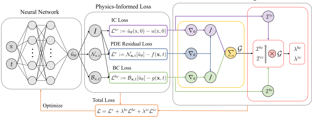
The proposed DB-PINN integrates inter-balancing and intra-balancing mechanisms to achieve the above two training goals. Specifically, inter-balancing aims to mitigate the gradient imbalance between the PDE residual loss and all condition-fitting losses based on gradient statistics by measuring the discrepancies between their gradient distributions. Meanwhile, intra-balancing acts between condition-fitting losses to alleviate the imbalance of fitting difficulty by assigning their weights proportionally to the degree of fitting difficulty. The proposed DB-PINN is illustrated in Figure 1.
3.1 Inter-Balancing Between PDE Residual Loss and Condition-Fitting Losses
Previous studies [Wang et al., 2022; Krishnapriyan et al., 2021; Wang et al., 2021] have revealed that the PDE residual loss generally exhibits dominance over the other loss terms, and this training imbalance severely hinders the training convergence and predictive accuracy of PINNs. To mitigate this imbalanced training, we first employ gradient statistics-based weighting methods to capture the gradient distribution discrepancies between PDE residual loss and every condition loss. Next, the overall gradient discrepancies can be derived by a summation. Thus, the total gradient ratio can be computed and considered as an aggregated weight. Specifically, we formulate the calculation procedure of the aggregated weight by adopting the mean magnitude of gradients (i.e., mean [Wang et al., 2021]) as a statistic:
where ∇θ denotes the gradient vector of the loss with respect to network parameters θ, |·| is the element-wise absolute value of the gradient vector, max denotes the maximum magnitude of gradients, and the overbar refers to the mean value of the gradient magnitudes. Equation (4) shows that the total gradient ratio is the sum of the maximum magnitude of the PDE residual loss's gradients divided by the mean magnitude of each weighted condition loss's gradients. Here the discrepancies in gradient distributions are measured by the mean magnitude which can be replaced by other statistical measures, such as standard deviation (std), kurtosis, etc [Maddu et al., 2022; Vemuri and Denzler, 2023; Deguchi and Asai, 2023]. As the aggregated weight characterizes the holistic relations between the PDE and conditions, it will be reallocated to each condition-fitting loss via intrabalancing among condition-fitting losses.
3.2 Intra-Balancing Among Condition-Fitting Losses
We further introduce intra-balancing among condition-fitting losses to encourage the model to prioritize fitting difficult conditions and prevent the continual over-allocation of learning resources to easy conditions. First, we define the condition-fitting loss vector Lt = [L1 , . . . , LM ]T ∈ RM+ , where the subscript t is the time step and the superscript denotes the i-th condition-fitting loss. To measure the model's fitting progress for different conditions, we introduce a difficulty index I which is defined as:
where Lt is the observed condition-fitting losses at time step t, and µLt is the average of the observed losses up to time t. The difficulty index I i t for the i-th condition reflects its inverse training rate, and thus it quantifies the fitting difficulty for the i-th condition. A larger value of I i t corresponds to a slower training rate, which indicates higher difficulty in fitting the i-th condition. Correspondingly, this condition loss should be assigned a larger weight. Therefore, we can allocate the aggregated weight proportionally to each conditionfitting loss based on the degree of fitting difficulty:
In this way, conditions with high fitting difficulty will be assigned large weights, as their entries in the difficulty indexes account for a substantial proportion. This weighting way for condition-fitting losses ensures that challenging conditions (high fitting difficulty) receive more attention, preventing an excessive focus on easier conditions. Hence, all conditionfitting losses can converge at a relatively balanced level.
Inner-Balancing for Solving PDEs with One Type of Condition Intra-balancing is absent for PDEs with a single specific type of condition (e.g., time-independent PDEs with only BCs). Hence, we introduce inner-balancing instead of intra-balancing to solve those PDEs with a type of condition. Specifically, we decompose the single-condition loss into two or multiple loss terms based on their inner characteristics (e.g., spatial differences, different variables, etc.):
Algorithm 1 DB-PINNs to dynamically adjust loss weights.
- 1: Consider a PINN with parameters θ to output ˆuθ(x, t). The total loss function is defined as: Ltotal = Lr + ∑Mi=1 λiLi , where Lr denotes the PDE residual loss, Li is i-th condition-fitting loss (e.g., the loss term of initial or boundary conditions, observational data, etc.), and λi is the corresponding loss weight of Li .
- 2: Define L0 = [L1 , . . . , LM ]T ∈ RM+ : a condition-fitting loss vector at time step t = 0.
- 3: Initialize the adaptive weights λi = 1, (i = 1, . . . ,M); difficulty indexes I0 = [1, . . . , 1]T ∈ RM+ and µL0 = L0 at time t = 0.
- 4: for t = 1 to max train steps do
- 5: Calculate Lr and Li using respective training points and obtain Lt = [L1 , . . . , LM ]T .
- 6: Calculate total gradient ratio: G = ∑Mi=1 max{|∇θLr |} |∇θλiLi | . (Inter-balancing)
- 7: Update µLt = (1 - 1t )µLt-1 + 1t Lt.
- 8: Calculate It = Lt µLt .
- 9: Calculate ˆλi = I i t ∑Mj=1 I j t × G. (Intra-balancing)
- 10: Update the weight λi = (1 - 1t )λi + 1t ˆλi .
- 11: Update the parameters θ = θ - η∇θLr - η ∑Mi=1 λi∇θLi .
- 12: end for
Ltotal = Lr + λLbc dec. = Lr + ∑i λiLi . The similar operations in equations (5) and (6) can be smoothly carried out to compute weights for each decomposed loss. As a result, inner-balancing enables DB-PINNs to extend beyond the scope of solving time-dependent PDEs.
3.3 Weight Update Strategy for DB-PINNs
Due to the stochastic nature of gradient descent updates, the instant weight values exhibit high variance. Existing gradient-based weighting methods usually adopt the Exponential Moving Average (EMA) strategy to update weights: λi = (1-α)λi +αˆλi , where α is a hyperparameter. However, we observed that this update strategy still fails to handle large variances, leading to frequent occurrences of abrupt spikes and even arithmetic overflow in the instant weight values, particularly when standard deviation or kurtosis is used as a statistical metric. To address this issue, we propose a robust freeof-tuning-hyperparameter loss weight update strategy. This strategy uses Welford's algorithm [Welford, 1962], an online estimate, to track the mean of the observed condition-fitting loss vector using the following update rules:
where µLt is updated using the previous observations µLt-1 and the current observation Lt. Likewise, the weight is also updated using the same update rules:
This strategy provides a computationally efficient way to estimate the mean from the history of observed losses and robustly update weights without additional hyperparameters. We summarize our proposed method in Algorithm 1.
4 Experiment
4.1 PDE Benchmarks
We perform the experiments on solving six PDE benchmarks to evaluate the effectiveness of DB-PINN. Due to the page limit, here we report the results of three PDEs. More experimental results are presented in the supplementary material.
Klein-Gordon Equation Klein-Gordon equation is a fundamental nonlinear equation in quantum mechanics and quantum field theory [Vemuri and Denzler, 2023]. We consider the Klein-Gordon equation with a boundary condition u(x, t) = x cos(5πt)+(xt)3 and initial conditions u(x, 0) = x and ut(x, 0) = 0:
Its exact solutions have the same analytical function as the boundary condition.
Wave Equation We consider the one-dimensional (1D) wave equation, which conventional PINNs struggle to solve due to its stiffness [Wang et al., 2022; McClenny and BragaNeto, 2020]. The wave equation with a boundary condition u(x, t) = 0 as well as the initial conditions u(x, 0) = sin(πx) + 0.5 sin(4πx) and ut(x, 0) = 0 is formulated as:
Its exact solutions are given:
Helmholtz Equation Helmholtz equation describes the propagation of waves with a specific frequency in acoustics, electromagnetics, and fluid dynamics fields. The PDE with a boundary condition u(x, y) = 0 is described as follows:
where the forcing term is
from which an analytical solution can be derived:
There is no initial condition, and thus no IC loss. To validate the effectiveness of DB-PINN on solving such a timeindependent PDE, we partition the four boundaries into two groups: the x-axis boundary and the y-axis boundary, and thus the BC loss consists of two loss terms. Inner-balancing between these two boundary loss terms aims to achieve a more balanced training for fitting boundary conditions of distinct variables.
4.2 Experimental Setting
We compare the performance of different weighting methods in PINNs. Specifically, equal weighting is used as a basic baseline. Uncertainty weighting [Xiang et al., 2022]
and SA-PINN [McClenny and Braga-Neto, 2023] are representative of the learning approach in weighting techniques. Regarding the PINNs using gradient-based weighting methods (denoted as GW-PINN), we adopt three different statistical measures which have been utilized in previous works: mean magnitude (mean) [Wang et al., 2021], standard deviation (std) [Maddu et al., 2022], and kurtosis [Vemuri and Denzler, 2023] for depicting the characteristics of gradient distribution. Accordingly, DB-PINN also has three implementations, each corresponding to a distinct gradient statistic used in inter-balancing.
We use hyperbolic tangent activation functions and the Adam optimizer with a learning rate of 0.001 as default. We choose the L2 relative error (L2RE) and mean absolute error (MAE) as evaluation metrics. In all cases below, the training process is iterated 10 times with random restarts. The average and standard deviation of errors are reported. More detailed experimental setups are shown in the supplementary material.
4.3 Main Results
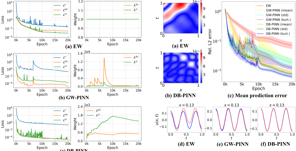
Insights Behind the Proposed DB-PINN and Its Benefits Figure 2 illustrates the training loss and weight curves over training epochs for EW, GW-PINN (std), and DB-PINN (std), revealing the limitations of GW-PINN and highlighting the advantages of DB-PINN. First, compared to EW, GW-PINN enlarges the gap between Lbc and Lic . This is because GWPINN consistently assigns a larger weight to Lbc than Lic , i.e., the curve of λbc is always above λic , even though the model already fits BC better than IC. Second, training losses usually exhibit variances, manifested as sharp fluctuations in the loss curves in Figure 2(a). However, GW-PINN is overly sensitive to instantaneous loss values, and the resulting weights undergo rapid volatility, leading to abrupt spikes. Ultimately, the model fails to reach the optimal. In contrast, DB-PINN effectively mitigates these two issues. In Figure 2(c), DB-PINN avoids BC overfitting and IC underfitting, and it ensures both condition losses steadily converge at almost the same rate to values below 10e-4. This is attributed to DB-PINN's capability to dynamically allocate robust weights guided by fitting difficulty with the proposed weight updating strategy. Please refer to the supplementary material for more results.
Klein-Gordon Equation Table 1 summarizes the results of PINNs using different weighting methods for solving the Klein-Gordon equation. Compared to equal weighting (EW), which has the largest errors, other methods significantly reduce prediction errors. This proves the importance of finding the optimal weights for better balancing several loss components in the PINN optimization. Regardless of the gradient statistics employed, our proposed DB-PINN consistently achieves more stable and accurate predictions than its counterpart, GW-PINN. DB-PINN (kurtosis) achieves the least prediction errors. Figure 3(a-b) shows the point-wise absolute prediction errors of EW and DB-PINN (kurtosis), and it indicates that DB-PINN yields the lower maximum errors. The snapshots in Figure 3(d-f) prove again that DB-PINN achieves the best prediction performance. Figure 3(c) shows that DB-PINN converges fastest and eventually achieves the least predictive errors.
| Klein-Gordon Equation | Wave Equation | Helmholtz Equation | |||||
|---|---|---|---|---|---|---|---|
| Method | L2RE (%) | MAE (%) | L2RE (%) | MAE (%) | L2RE (%) | MAE (%) | |
| Equal weighting | 7.272 ± 3.566 | 2.415 ± 1.320 | 39.870 ± 1.612 | 16.071 ± 0.671 | 7.174 ± 2.434 | 2.257 ± 0.757 | |
| Uncertainty weighting | 1.450 ± 0.705 | 0.478 ± 0.227 | 32.572 ± 3.486 | 13.094 ± 1.386 | 0.845 ± 0.888 | 0.314 ± 0.368 | |
| SA-PINN | 3.696 ± 1.085 | 1.193 ± 0.318 | 33.867 ± 2.085 | 13.568 ± 0.826 | 2.413 ± 0.418 | 0.753 ± 0.159 | |
| GW-PINN | mean | 2.062 ± 0.890 | 0.690 ± 0.293 | 2.126 ± 0.360 | 0.916 ± 0.154 | 0.796 ± 0.125 | 0.188 ± 0.026 |
| std | 1.848 ± 1.455 | 0.623 ± 0.494 | 8.093 ± 10.072 | 3.369 ± 4.117 | 0.270 ± 0.089 | 0.105 ± 0.037 | |
| kurtosis | 1.262 ± 0.403 | 0.421 ± 0.134 | 17.361 ± 7.938 | 7.630 ± 3.434 | 0.331 ± 0.071 | 0.113 ± 0.034 | |
| mean | 0.885 ± 0.257 | 0.297 ± 0.092 | 0.852 ± 0.193 | 0.373 ± 0.084 | 0.180 ± 0.023 | 0.055 ± 0.008 | |
| DB-PINN std | 0.767 ± 0.112 | 0.254 ± 0.041 | 0.292 ± 0.129 | 0.128 ± 0.056 | 0.235 ± 0.065 | 0.093 ± 0.025 | |
| kurtosis | 0.636 ± 0.132 | 0.214 ± 0.049 | 0.715 ± 0.507 | 0.293 ± 0.214 | 0.140 ± 0.018 | 0.052 ± 0.009 | |
(c) DB-PINN
Figure 2: Loss and weight curves during the training on solving the Klein-Gordon equation.
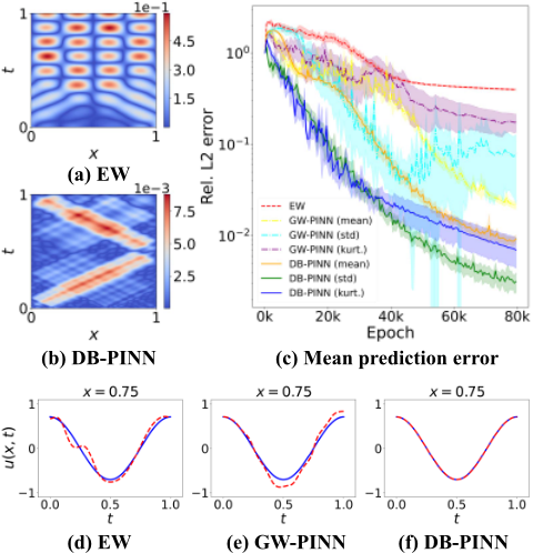
Wave Equation Table 1 compares the performance of different methods for solving the wave equation. Equal weighting struggles to solve this PDE with the relative L2 error around 40%. Uncertainty weighting and SA-PINN achieve a slight improvement in accuracy. GW-PINN enlarges the performance gap with the baseline but exhibits unstable performance related to the statistical metrics. Thus, the choice of gradient statistics plays a significant role in the performance of GW-PINN when solving more intricate stiff PDEs. Fortunately, DB-PINN exhibits a significant advantage in that the performance gaps induced by the employed gradient statistics are greatly reduced. Specifically, DB-PINN consistently obtains the best prediction performance among these different weighting methods. Figure 4(a-b) visually compares the performance of EW and DB-PINN (kurtosis). DB-PINN achieves better prediction accuracy, which is also proved by the comparison in Figure 4(d-f). Figure 4(c) shows that DBPINN has a fast convergence speed and stable predictive performance with low errors.
Figure 3: The Klein-Gordon equation. (a-b) Point-wise absolute errors. (c) Mean prediction error curves. (d-f) Comparison between reference solutions (blue) and predictions (red).
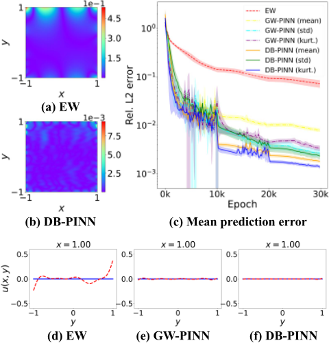
Helmholtz Equation Table 1 reports the results for solving the Helmholtz PDE. Compared with GW-PINN using identical statistics, DB-PINN attains lower errors. DB-PINN (kurtosis) yields the least errors with the L2RE of 0.140% and MAE of 0.052%. Hence, the effectiveness of DB-PINN in solving time-independent PDEs also has been validated. Figure 5(a-b) indicates that DB-PINN (kurtosis) has the lowest maximum errors. Figure 5(d-f) shows the snapshots of prediction at the boundary x = 1.00. DB-PINN (kurtosis) achieves predictions that closely match reference solutions. Figure 5(c) shows that DB-PINN exceeds GW-PINN in both convergence speed and prediction accuracy.
4.4 Ablation Study
Dual-Balancing We conduct ablation studies on solving the Klein-Gordon equation to evaluate the respective contribution of the dual-balancing and the weight update strategy in DB-PINN. Table 2 reports the results of the ablation study about the dual-balancing mechanism in DB-PINN. Our approach without inter- and intra-balancing is denoted as 'DBPINN w/o balancing', which is equivalent to GW-PINN with the proposed weight update strategy. 'DB-PINN-Avg' refers to the DB-PINN without intra-balancing, which allocates the average of the aggregated weight to each condition loss. Regardless of any one of the statistical metrics, 'DB-PINN w/o balancing' consistently achieves inferior performance than DB-PINN in Table 1. Notice that 'DB-PINN-Avg' obtains poorer accuracy than DB-PINN, which justifies the necessity of balancing the training to learn multiple conditions with different levels of fitting difficulty. Therefore, inter-balancing and intra-balancing are indispensable to addressing two imbalance issues, constituting the dual-balancing mechanism collaboratively.
| Method | Stats | L2RE (%) | MAE (%) |
|---|---|---|---|
| DB-PINN w/o balancing | mean std kurt. | 1.095 ± 0.142 0.969 ± 0.204 0.797 ± 0.122 | 0.376 ± 0.049 0.329 ± 0.070 0.267 ± 0.043 |
| DB-PINN-Avg | mean std kurt. | 0.985 ± 0.175 0.899 ± 0.152 0.776 ± 0.113 | 0.336 ± 0.062 0.302 ± 0.052 0.263 ± 0.038 |
| Method | α | Stats | L2RE (%) | MAE (%) |
|---|---|---|---|---|
| DB-PINN w/ EMA | 0.5 0.2 | mean std kurt. mean | 1.486 ± 0.534 1.337 ± 0.367 1.205 ± 0.273 1.305 ± 0.474 | 0.490 ± 0.163 0.451 ± 0.124 0.405 ± 0.092 |
| 0.01 | std kurt. mean std kurt. | 1.182 ± 0.294 1.112 ± 0.248 1.034 ± 0.306 0.913 ± 0.133 0.859 ± 0.193 | 0.440 ± 0.164 0.402 ± 0.098 0.378 ± 0.086 0.347 ± 0.102 0.307 ± 0.046 0.292 ± 0.067 |
Weight Update Strategy To evaluate the proposed weight update strategy, we replace it with EMA, denoted as 'DBPINN w/ EMA'. The results are reported in Table 3. As there is a hyperparameter α in EMA, we run 'DB-PINN w/ EMA' with α = 0.5, α = 0.2, and α = 0.01, respectively. Table 3 indicates that the performance of 'DB-PINN w/ EMA' is very susceptible to α. The accuracy of 'DB-PINN w/ EMA' increases along with the descending α. This reminds us to carefully select the value of α when using EMA, but undoubtedly, it can lead to the heavy consumption of computational resources because of trials and errors in tuning this hyperparameter. Importantly, 'DB-PINN w/ EMA' steadily performs worse than DB-PINN, which demonstrates the superiority of the weight update strategy over EMA.
5 Conclusion
In this work, we propose DB-PINNs to adaptively adjust the loss weights in PINNs by combining inter-balancing (to mitigate the gradient imbalance between PDE residual loss and condition losses) with intra-balancing (to address the imbalance in fitting difficulty among different condition losses). We further introduce a robust weight update strategy to tackle the large variance in weight values for stable training. Experimental results show that DB-PINN consistently exceeds GWPINN in both convergence speed and prediction accuracy.
@inproceedings{ijcai2025p797,
  title     = {Dual-Balancing for Physics-Informed Neural Networks},
  author    = {Zhou, Chenhong and Chen, Jie and Yang, Zaifeng and Png, Ching Eng},
  booktitle = {Proceedings of the Thirty-Fourth International Joint Conference on
               Artificial Intelligence, {IJCAI-25}},
  publisher = {International Joint Conferences on Artificial Intelligence Organization},
  editor    = {James Kwok},
  pages     = {7164--7172},
  year      = {2025},
  month     = {8},
  note      = {Main Track},
  doi       = {10.24963/ijcai.2025/797},
  url       = {https://doi.org/10.24963/ijcai.2025/797},
}
TY - CPAPER TI - Dual-Balancing for Physics-Informed Neural Networks AU - Zhou, Chenhong AU - Chen, Jie AU - Yang, Zaifeng AU - Png, Ching Eng T2 - Proceedings of the Thirty-Fourth International Joint Conference on Artificial Intelligence, IJCAI-25 PB - International Joint Conferences on Artificial Intelligence Organization PY - 2025 SP - 7164 EP - 7172 DO - 10.24963/ijcai.2025/797 UR - https://doi.org/10.24963/ijcai.2025/797 ER -Copied
Machine-readable versions of this paper, for tools and AI agents:





