
KP-PINNs: Kernel Packet Accelerated Physics Informed Neural Networks
Proceedings of the Thirty-Fourth International Joint Conference on Artificial Intelligence. Main Track. Pages 7904-7912.
https://doi.org/10.24963/ijcai.2025/879
Keywords
- Multidisciplinary Topics and Applications: MTA: Physical sciences
- Machine Learning: ML: Deep learning architectures
- Machine Learning: ML: Applications
Abstract
Differential equations are involved in modeling many engineering problems. Many efforts have been devoted to solving differential equations. Due to the flexibility of neural networks, Physics Informed Neural Networks (PINNs) have recently been proposed to solve complex differential equations and have demonstrated superior performance in many applications. While the L2 loss function is usually a default choice in PINNs, it has been shown that the corresponding numerical solution is incorrect and unstable for some complex equations. In this work, we propose a new PINNs framework named Kernel Packet accelerated PINNs (KP-PINNs), which gives a new expression of the loss function using the reproducing kernel Hilbert space (RKHS) norm and uses the Kernel Packet (KP) method to accelerate the computation. Theoretical results show that KP-PINNs can be stable across various differential equations. Numerical experiments illustrate that KP-PINNs can solve differential equations effectively and efficiently. This framework provides a promising direction for improving the stability and accuracy of PINNs-based solvers in scientific computing.
- [Abramowitz and Stegun, 1968] Milton Abramowitz and Irene A Stegun. Handbook of mathematical functions with formulas, graphs, and mathematical tables, volume 55. US Government printing office, 1968.
- [Adams and Fournier, 2003] Robert A Adams and John JF Fournier. Sobolev Spaces. Academic Press, 2nd edition, 2003.
- [Aliakbari, 2023] Maryam Aliakbari. Physics informed neu- ral networks to solve forward and inverse fluid flow and heat transfer problems. PhD thesis, Northern Arizona Uni- versity, 2023.
- [Atkinson et al., 2009] Kendall Atkinson, Weimin Han, and David E Stewart. Numerical solution of ordinary differen- tial equations, volume 81. John Wiley & Sons, 2009.
- [Bramble and Schatz, 1970] James H Bramble and Alfred H Schatz. Rayleigh-ritz-galerkin methods for dirichlet's problem using subspaces without boundary conditions. Communications on Pure and Applied Mathematics, 23(4):653-675, 1970.
- [Byrd et al., 1995] Richard H Byrd, Peihuang Lu, Jorge No- cedal, and Ciyou Zhu. A limited memory algorithm for bound constrained optimization. SIAM Journal on scien- tific computing, 16(5):1190-1208, 1995.
- [Chen et al., 2022] Haoyuan Chen, Liang Ding, and Rui Tuo. Kernel packet: An exact and scalable algo- rithm for gaussian process regression with matérn corre- lations. Journal of machine learning research, 23(127):1- 32, 2022.
- [Davis, 2006] Timothy A Davis. Direct methods for sparse linear systems. SIAM, 2006.
- [Deschamps, 1981] Georges A Deschamps. Electromagnet- ics and differential forms. Proceedings of the IEEE, 69(6):676-696, 1981.
- [Ding et al., 2019] Liang Ding, Simon Mak, and CF Wu. Bdrygp: a new gaussian process model for incorporating boundary information. arXiv preprint arXiv:1908.08868, 2019.
- [Ding et al., 2020] Liang Ding, Lu Zou, Wenjia Wang, Shahin Shahrampour, and Rui Tuo. High-dimensional non-parametric density estimation in mixed smooth sobolev spaces. arXiv preprint arXiv:2006.03696, 2020.
- [Dũng and Nguyen, 2021] Dinh Dũng and Van Kien Nguyen. Deep relu neural networks in high-dimensional approximation. Neural Networks, 142:619-635, 2021.
- [Evans and Souganidis, 1989] Lawrence C Evans and Pana- giotis E Souganidis. A pde approach to geometric optics for certain semilinear parabolic equations. Indiana Uni- versity mathematics journal, 38(1):141-172, 1989.
- [Evans, 2022] Lawrence C Evans. Partial differential equa- tions, volume 19. American Mathematical Society, 2022.
- [Forootani et al., 2024] Ali Forootani, Harshit Kapadia, Sridhar Chellappa, Pawan Goyal, and Peter Benner. Gs- pinn: Greedy sampling for parameter estimation in partial differential equations. arXiv preprint arXiv:2405.08537, 2024.
- [Ghergu and Radulescu, 2011] Marius Ghergu and Vicentiu Radulescu. Nonlinear PDEs: Mathematical models in bi- ology, chemistry and population genetics. Springer Sci- ence & Business Media, 2011.
- [Guo, 2022] Qing Guo. Optimal robust control of electro- hydraulic system based on hamilton-jacobi-bellman solu- tion with backstepping iteration. IEEE Transactions on Control Systems Technology, 31(1):459-466, 2022.
- [Haitsiukevich and Ilin, 2022] Katsiaryna Haitsiukevich and Alexander Ilin. Improved training of physics-informed neural networks with model ensembles. arXiv preprint arXiv:2204.05108, 2022.
- [Han et al., 2018] Jiequn Han, Arnulf Jentzen, and Weinan E. Solving high-dimensional partial differential equations using deep learning. Proceedings of the National Academy of Sciences, 115(34):8505-8510, 2018.
- [Hochmuth et al., 2000] Reinhard Hochmuth, Stephan Knapek, and Gerhard Zumbusch. Tensor products of Sobolev spaces and applications. Citeseer, 2000.
- [Hu et al., 2021] Zheyuan Hu, Ameya D Jagtap, George Em Karniadakis, and Kenji Kawaguchi. When do extended physics-informed neural networks (xpinns) improve gen- eralization? arXiv preprint arXiv:2109.09444, 2021.
- [Isachenko et al., 1980] Viktor Pavlovich Isachenko, Var- vara Aleksandrovna Osipova, and Aleksandr Semenovič Sukomel. Heat transfer. Nirali Prakashan, 1980.
- [Jagtap et al., 2020] Ameya D Jagtap, Kenji Kawaguchi, and George Em Karniadakis. Adaptive activation functions ac- celerate convergence in deep and physics-informed neural networks. Journal of Computational Physics, 404:109136, 2020.
- [Kaltenbacher, 2018] Manfred Kaltenbacher. Computational acoustics. Springer, 2018.
- [Karniadakis et al., 2021] George Em Karniadakis, Ioan- nis G Kevrekidis, Lu Lu, Paris Perdikaris, Sifan Wang, and Liu Yang. Physics-informed machine learning. Nature Re- views Physics, 3(6):422-440, 2021.
- [Kianiharchegani, 2023] Elham Kianiharchegani. Data- Driven Exploration of Coarse-Grained Equations: Har- nessing Machine Learning. PhD thesis, The University of Western Ontario (Canada), 2023.
- [Kingma and Ba, 2014] Diederik P Kingma and Jimmy Ba. Adam: A method for stochastic optimization. arXiv preprint arXiv:1412.6980, 2014.
- [Kreyszig, 2007] Erwin Kreyszig. Advanced Engineering Mathematics 9th Edition with Wiley Plus Set, volume 334.
- [Kühn et al., 2015] Thomas Kühn, Winfried Sickel, and Tino Ullrich. Approximation of mixed order sobolev func- tions on the d-torus: asymptotics, preasymptotics, and d- dependence. Constructive Approximation, 42:353-398, 2015.
- [Li et al., 2022] Ying Li, Longxiang Xu, and Shihui Ying. Dwnn: Deep wavelet neural network for solving partial differential equations. Mathematics, 10(12):1976, 2022.
- [Lin et al., 2022] Guang Lin, Yating Wang, and Zecheng Zhang. Multi-variance replica exchange sgmcmc for in- verse and forward problems via bayesian pinn. Journal of Computational Physics, 460:111173, 2022.
- [Muyskens et al., 2024] Amanda Muyskens, Benjamin W Priest, Imene R Goumiri, and Michael D Schneider. Iden- tifiability and sensitivity analysis of kriging weights for the matern kernel. arXiv preprint arXiv:2410.08310, 2024.
- [Nguyen et al., 2023] Van Giang Nguyen, Van Linh Nguyen, Sungho Jung, Hyunuk An, and Giha Lee. Exploring the power of physics-informed neural networks for accurate and efficient solutions to 1d shallow water equations. Jour- nal of Korea Water Resources Association, 56(12):939- 953, 2023.
- [Ragheb, 1976] M Ragheb. Computational fluid dynamics. mragheb Website, Available Online at https://mragheb. com/NPRE, 20475, 1976. Link
- [Raissi et al., 2019] Maziar Raissi, Paris Perdikaris, and Karniadakis. Physics-informed neural networks: A deep learning framework for solving forward and inverse prob- lems involving nonlinear partial differential equations. Journal of Computational physics, 378:686-707, 2019.
- [Shin et al., 2023] Yeonjong Shin, Zhongqiang Zhang, and George Em Karniadakis. Error estimates of residual min- imization using neural networks for linear pdes. Journal of Machine Learning for Modeling and Computing, 4(4), 2023.
- [Sieniutycz, 2000] Stanislaw Sieniutycz. Hamilton-jacobi- bellman framework for optimal control in multistage en- ergy systems. Physics Reports, 326(4):165-258, 2000.
- [Son et al., 2021] Hwijae Son, Jin Woo Jang, Woo Jin Han, and Hyung Ju Hwang. Sobolev training for physics informed neural networks. arXiv preprint arXiv:2101.08932, 2021.
- [Wang and Jing, 2022] Wenjia Wang and Bing-Yi Jing. Gaussian process regression: Optimality, robustness, and relationship with kernel ridge regression. Journal of Ma- chine Learning Research, 23(193):1-67, 2022.
- [Wang et al., 2020] Wenjia Wang, Rui Tuo, and CF Jeff Wu. On prediction properties of kriging: Uniform error bounds and robustness. Journal of the American Statistical Asso- ciation, 115(530):920-930, 2020.
- [Wang et al., 2022] Chuwei Wang, Shanda Li, Di He, and Liwei Wang. Is L 2 physics-informed loss always suit- able for training physics-informed neural network? arXiv preprint arXiv:2206.02016, 2022.
- [Wanner and Hairer, 1996] Gerhard Wanner and Ernst Hairer. Solving ordinary differential equations II, volume 375. Springer Berlin Heidelberg New York, 1996.
- [Wendland, 2004] Holger Wendland. Scattered data approx- imation, volume 17. Cambridge university press, 2004.
- [Witte and Reisinger, 2011] Jan Hendrik Witte and Christoph Reisinger. A penalty method for the nu- merical solution of hamilton-jacobi-bellman (hjb) equations in finance. SIAM Journal on Numerical Analysis, 49(1):213-231, 2011.
- [Yan et al., 2025] Lei Yan, Qiulei Wang, Gang Hu, Wenli Chen, and Bernd R Noack. Deep reinforcement cross- domain transfer learning of active flow control for three- dimensional bluff body flow. Journal of Computational Physics, 529:113893, 2025.
- [Yong and Zhou, 2012] Jiongmin Yong and Xun Yu Zhou. Stochastic controls: Hamiltonian systems and HJB equa- tions, volume 43. Springer Science & Business Media, 2012.
- [Yu et al., 2022] Jeremy Yu, Lu Lu, Xuhui Meng, and George Em Karniadakis. Gradient-enhanced physics- informed neural networks for forward and inverse pde problems. Computer Methods in Applied Mechanics and Engineering, 393:114823, 2022.
- [Yuan et al., 2022] Lei Yuan, Yi-Qing Ni, Xiang-Yun Deng, and Shuo Hao. A-pinn: Auxiliary physics informed neural networks for forward and inverse problems of nonlinear integro-differential equations. Journal of Computational Physics, 462:111260, 2022.
- [Zhang et al., 2024] Weiwei Zhang, Wei Suo, Jiahao Song, and Wenbo Cao. Physics informed neural networks (pinns) as intelligent computing technique for solving partial dif- ferential equations: Limitation and future prospects. arXiv preprint arXiv:2411.18240, 2024.
References were extracted automatically from the PDF and may contain errors.
Full text extracted automatically from the PDF; figures, tables and equations may differ. The PDF is the version of record.
1 Introduction
Differential equations, including ordinary differential equations (ODEs) and partial differential equations (PDEs), are widely applied in engineering for modelling, analyzing, and optimizing dynamic systems [Kreyszig, 2007]. They provide a mathematical framework for describing natural phenomena and solving complex problems. Differential equations are widely used in simulating fluid dynamics [Ragheb, 1976], electromagnetics [Deschamps, 1981], heat transfer [Isachenko et al., 1980] and acoustics [Kaltenbacher, 2018] Differential equations solutions are crucial for accurately predicting and optimizing the behaviour of dynamic systems, ensuring effective design and operation in engineering applications.
˚Corresponding author.
Because analytical solutions of differential equations are often difficult to obtain in practice, researchers seek numerical methods instead. For example, Euler's method and Runge-Kutta method [Atkinson et al., 2009] can be applied to solving ODEs, and finite element method (FEM), finite difference method (FDM), finite volume method (FVM), and spectral methods can be used to solve PDEs. These methods provide a foundation for solving various differential equations encountered in engineering and scientific applications. However, such methods require substantial computational resources and memory, particularly in high-dimensional or complex physical scenarios. Moreover, they lack flexibility, as adapting to different physical problems or parameter changes often needs significant model reconfiguration [Karniadakis et al., 2021].
With the development of deep learning, Physics informed neural networks (PINNs) incorporate physical laws into training neural networks to solve differential equations [Kianiharchegani, 2023], particularly PDEs, by effectively combining deep learning with domain-specific knowledge. PINNs have strong flexibility and can be effectively combined with existing traditional methods. However, PINNs can lead to incorrect solutions for some complex PDEs, affecting the accuracy of the solutions obtained [Zhang et al., 2024]. Several methods are proposed to address this issue. For example, [Haitsiukevich and Ilin, 2022] used ensemble agreement for domain expansion, and the improved algorithm can make the training of PINNs more stable. [Hu et al., 2021] theoretically analyzed the convergence and generalization of extended PINNs. [Yu et al., 2022] proposed gradient-enhanced PINNs, which utilize the gradient information of PDEs residuals and embed the gradient into the loss function to improve the effectiveness of solving PDEs. Other works include [Nguyen et al., 2023; Forootani et al., 2024; Aliakbari, 2023; Yuan et al., 2022; Lin et al., 2022].
However, it has been noticed that the original PINNs are not stable [Wang et al., 2022], due to the default L2 loss function. To address the instability of the original PINNs, [Wang et al., 2022] proposed the L8 loss function and proposed an adversarial training method. However, the computation of L8 norm is complicated, and the adversarial training is timeconsuming. Another class of loss functions is based on the Sobolev norm, which is proposed by [Son et al., 2021], and the corresponding method is named as Sobolev-PINNs. However, the computation of the Sobolev norm in Sobolev-PINNs is complex, and accurate derivative information is hard to get.
In this work, we propose a novel form of loss function using the Reproducing Kernel Hilbert Space (RKHS) norm. Under specific choice of the kernel function, the RKHS norm is equivalent to the (tensored) Sobolev norm, thus addressing the stability issue of the original PINNs. The proposed method can also avoid directly computing the derivative because the RKHS norm of a function can be approximated by the RKHS norm of its interpolation, while the later has a close form. To compute the RKHS norm, we employ Kernel Packet (KP) method [Chen et al., 2022], which can efficiently compute the inverse of the kernel matrix. Therefore, KP accelerated PINNs (KP-PINNs) can solve differential equations effectively and efficiently. We also provide theoretical guarantee for our proposed method.
The rest is organized as follows. Section 2 briefly introduces differential equations, PINNs and KP. Section 3 analyses the proposed KP-PINNs algorithm. Section 4 gives some theoretical results. Section 5 shows four numerical examples to demonstrate the performance of the KP-PINNs algorithm. Section 6 gives this research's discussion and future work.
2 Preliminaries
2.1 Differential Equations
Differential equations are mathematical equations that describe the relationship between a function and its derivatives, representing how a quantity changes over time or space. They are broadly classified into ordinary differential equations (ODEs), which involve functions of a single variable, and partial differential equations (PDEs), which involve functions of multiple variables. Differential equations are foundational in modeling dynamic systems and natural phenomena. By capturing the principles of change and interaction, they provide powerful tools for analyzing and solving complex problems. In general, a differential equation system can be expressed [Evans, 2022] by:
"
where Ω is an open domain with boundary BΩ, Lθ represents a partial differential operator, Bθ denotes the boundary condition, fθ and gθ are two known functions defined on Ω and BΩ, respectively, θ is the parameter, and u is an unknown function. The goal of solving a differential equation system is to find u such that (1) holds. Usually, (1) is called ODE if d " 1, and PDE if d ą 1. An example of PDEs is the second-order linear PDE, with
x " px1, ..., xdqJ P Rd , and the parameters are αi,j, βk, γ for i, j, k P t1, . . . , du.
Besides the linear PDEs, where Lθ is a linear differential operator, nonlinear PDEs, in which the solution or its derivatives appear nonlinearly, make them more complex to solve compared to linear PDEs. Because of the flexibility of nonlinear PDEs, it has been widely applied in fluid dynamics [Yan et al., 2025], optics [Evans and Souganidis, 1989], and biology [Ghergu and Radulescu, 2011]. One particular example is the Hamilton-Jacobi-Bellman (HJB) equations, which are widely applied in electro-hydraulic systems [Guo, 2022], energy systems [Sieniutycz, 2000] and finance [Witte and Reisinger, 2011]. The HJB equations characterise the optimal control strategy for a dynamic system under certain constraints and objectives. Specifically, the form of the HJB equations [Yong and Zhou, 2012] can be expressed by
where upx, tq is the value function, kpx, tq is the given control function, rpx, kq is the cost rate during the process and gpxq is the final cost at the terminal state [Wang et al., 2022]. If the cost rate function is rpx, kq " a1|k1|b1 `¨ ¨ ¨`ad|kd|bd ´ hpx, tq then the HJB equations can be expressed [Yong and Zhou, 2012] as
$'&'%
where Ai " paibiq´ 1 bi´1 ´ aipaibiq´ bi bi´1 ą 0 with ci " bi bi´1 ą 1, L0u :" B Bt u ´ ∆u is a linear operator, and ˜ LHJBu :" L0u ` řdi"1 Ai|Biu|ci is a nonlinear operator.
In the forward problem of differential equations, the goal is to obtain a function u such that (1) is satisfied, where all the operators and functions Lθ, Bθ, hθ and gθ are known. In practice, there are many scenarios where the parameter θ is unknown and needs to be estimated based on the equation form and observed data. This is called inverse problems, where the goal is to recover the parameters. In this work, we consider both forward problems and inverse problems.
2.2 Physics Informed Neural Networks
Physics informed neural networks (PINNs) provide a flexible way for numerically solving the differential equation systems (1).
For notational convenience, let
Clearly, u is the solution to (1) if and only if h1 " h2 " 0. Therefore, for the forward problem, it is natural to minimize the loss function
which was considered by [Raissi et al., 2019]. Choose xi P Ω, i " 1, ...,NL and si P BΩ, i " 1, ...,NB. Then (6) can be approximated by
with
PINNs use a deep neural network, denoted by unn, to minimize the loss function in (7).
For the inverse problems, suppose that we have observed function values at points xi P Ω, i " 1, ...,NL and si P BΩ, i " 1, ...,NB, denoted by udpxi q and udpsi q, respectively. We define the loss function in the inverse problem as
where Losspuq is as in (7), and
with h3 " u ´ ud. The goal of solving an inverse problem is to solve
where Θ is the parameter space. In practice, the minimizers of the loss functions in both forward and inverse problems can be found via optimization algorithms such as Adam [Kingma and Ba, 2014] and L-BFGS [Byrd et al., 1995].
2.3 Kernel Packet
Our proposed method relies on Kernel Packet (KP), which was proposed in [Chen et al., 2022]. In functional analysis, a Hilbert space of functions is termed a Reproducing Kernel Hilbert Space (RKHS) if the evaluation is a continuous linear operator at any point within the space. Assume that Ω Ă Rd is compact with Lipschtiz boundary, and Φ : ΩˆΩ Ñ R is a symmetric positive definite kernel function [Wang and Jing, 2022; Wang et al., 2020]. Define the linear space
and equip this space with the bilinear form
C
where the RKHS NΦpΩq generated by kernel Φ is defined as the closure of FΦpΩq under the inner product x¨, ¨yΦ. The norm of NΦpΩq is ||f||NΦpΩq " bxf, fyNΦpΩq, where x¨, ¨yNΦpΩq is induced by x¨, ¨yΦ.
Let x1, ..., xn P Ω Y BΩ be the points of interest. KP provides an efficient way to compute the inverse of the kernel matrix K :" pΦpxj, xkqqjk P Rnˆn , which is essential in the application of the RKHSs, for example, prediction in kernel ridge regression, and computing the posterior variance in Bayesian optimization. In KP, it is assumed that the kernel function Φ is a Mat´ern kernel function [Abramowitz and Stegun, 1968] as
where ℓ ą 0 is the scale parameter, and ν is the half integer smoothness parameter. For example, when ν is equal to 12 , the corresponding kernel function is Φ12 pxj, xkq " exp p´ℓ|xj ´ xk|q. The Mat´ern kernel function is widely applied in practice; see [Muyskens et al., 2024] for example.
For a moment, let us consider the case d " 1. Without loss of generality, assume x1 ă x2 ă . . . ă xn. A nonzero function ϕ is termed an s degree KP if it can admit the representation as
with the support of ϕ being the interval rx1, xns. In (11), Aj is the coefficients of Φpx, xjq, which can be obtained by solving the following linear systems:
where l " 0, ..., s´3 2 , δ " ˘1, c2 " 2ν ℓ2 (ν and ℓ are the smoothness parameter and scale parameter of Mat´ern kernel function respectively). By (11), we have AK " ϕpxq, and the inverse of the kernel matrix can be computed by
where x " px1, x2, . . . , xnqJ is the input vector, and the pi, jqth entry of ϕpXq and A are ϕjpxiq and the i element of Aj, respectively.
It has been shown in [Chen et al., 2022] that both A and ϕpxq are sparse banded matrices, hence the computation of K´1 can be fast. Specifically, [Chen et al., 2022] showed that computing A and ϕpxq needs only Opp2ν ` 2q3nq computation time and requires storage space of Opp2ν`2qnq, where ν is usually small in most practical applications. LU decomposition [Davis, 2006] can be applied for solving rϕpxqs´1 , and [Chen et al., 2022] showed that the total computation time is only Opn2 q.
If d ą 1, i.e., the input X is multi-dimensional, then special structure of the input points X " px1, x2, ..., xdq is needed. KP requires the input points to be tensor-like, that is, the input points can be described as the Cartesian combination of multiple one-dimensional point collections. Specifically, XFG " ŚNi"1 xpiq , where each xpiq represents a distinct one-dimensional point collection. With tensor-like input points, K can be decomposed into Kronecker products as
where Kxi " pΦpxij , xikqq, 1 ď i ď d, 1 ď j, k ď ni, ni is the number of points for dimension i and thus the dimension of K is n ˆ n, where n " śdi"1 ni. Then the inverse K can be directly computed by
where each K´1 xi can be computed using one-dimensional KP. Putting all things together, we obtain
whose computation time is still Opn2 q.
3 KP Accelerated PINNs
In this section, we introduce the proposed method, KP accelerated PINNs (KP-PINNs). Instead of using L2 loss in (6), which was shown to be unstable in some specific PDE systems, we consider tensor Sobolev norm. The tensor Sobolev space Hν T pΩq [Hochmuth et al., 2000] is defined as the set of functions f : ΩÑR satisfying
where ||f||HνT pΩq is the norm on Hν T pΩq, explicitly defined via the Fourier transform as
where ˜ fpωq represents the Fourier transform of f. We define the loss function with tensor Sobolev norm as
where λ ą 0 is a tuning parameter that balances the weights between the difference between the space and its boundary, and uNN is the predicted value obtained from the neural network. However, directly computing the tensor Sobolev norm may be time-consuming and inaccurate. By the equivalence between the RKHS norm and tensor Sobolev norm, we modify the loss function (19) to
where NΦνT is tensor RKHS, i.e. the RKHS generated by ΦνT pxq " śdi"1 Φν pxiq. Tensor RKHS and Sobolev space are widely considered for complexity reduction in highdimensional spaces [Ding et al., 2020; K¨uhn et al., 2015; D˜ung and Nguyen, 2021].
Computing the loss function in (20) can be efficient via KP. Specifically, let
and we consider ||h1NN||2NΦνT pΩq " ||LuNN ´ f||2NΦνT pΩq first. Based on the Theorem 11.23 in [Wendland, 2004], ||h1NN||2NΦνT pΩq can be approximated by
where yh1 " ph1NNpx1 q, ..., h1NNpxnqq and x1 , ..., xn P Rd means all the training data. K is as in (14). The other term ||h2NN||2NΦνT pBΩq can be approximated in a similar manner.
Algorithm 1 KP-PINNs
Input: PDE systems (1), iterations niter, known points Output: Approximated solution ˆupxq and equations' parameters (if inverse problem)
- 1: Initialize neural network parameters.
- 2: while i ă niter do
- 3: Forward pass and compute the predicted value.
- 4: Compute derivatives using automatic differentiation.
- 5: Compute A and ϕpxq by (12) and (11).
- 6: Compute the loss of KP-PINNs based on (23).
- 7: Update parameters.
- 8: end while
With (13), (16) and approximation (22), the loss function (20) can be approximated by:
By KP method introduced in Section 2.3, LossNΦνT can be easily computed.Some well-established optimization algorithms, such as Adam or L-BFGS, can be used to minimize the loss effectively. The KP-PINNs algorithm is summarized in Algorithm 1. For the inverse problem, comparing (7) and (8), it can be seen that the loss function of the inverse problem has more LossDpuq part. For this part, the computation of the RKHS norm is similar to the analysis above. In this way, the KP-PINNs algorithm can effectively solve both forward and inverse problems.
4 Theoretical Results
In this section, we analyze the stability of PDEs solved with the loss function (19), or equivalently (20). The stability of a PDE system is defined as follows [Wang et al., 2022].
Definition 1 (Stability of PDEs [Wang et al., 2022]). Suppose Z1,Z2, and Z3 are three Banach spaces. For the exact solution u˚ pxq and the predicted solution u, if for ||Lu´f ||Z1 , ||Bu´g||Z2 Ñ 0, it has ||u˚´u||Z3 " Op||Lu´ f||Z1 ` ||Bu ´ g||Z2 q, then the PDEs (1) is pZ1,Z2,Z3qstable.
Stability defined in Definition 1 provides a theoretical guarantee for solving a PDE. Specifically, if the loss function is ||Lu´f||Z1 `||Bu´g||Z2 , thenminimizing the loss function can ensure the convergence of the solution under Z3-norm. In this section, we consider two classes of PDEs: second-order linear elliptic equations and Hamilton-Jacobi-Bellman (HJB) equations. We start with the second-order linear elliptic equations satisfying the following assumption. While in the previous section, we considered the parameters of the PDE as constants, here we extend the analysis to a more general case, where the parameters are functions. This allows us to establish the theoretical results in a broader context.
Assumption 1. Suppose in (1), the operator L " řdi,j"1 ai,jpxqBxi Bxj ` řdi"1 bipxqBxi ` cpxq and B is the identity operator. The functions ai,j P C 2 satisfy the uniformly elliptic condition. In addition, the only solution with zero input data is the zero solution.
Lemma 1 (Theorem 2.1 in [Bramble and Schatz, 1970]). In addition to Assumption (1), assume that L is with C 8 coefficients, defined on C 8 bounded domain Ω on Rd . For any real number l, ||u||Hl pΩq ď C ´||Lu||Hl´2 pΩq ` ||u||Hl´ 1 2 pBΩq¯ for all u P C 8p¯Ωq, where ¯Ω is a closure of Ω and C is independent of u.
Theorem 1 (Stability of second-order linear elliptic equation). Suppose the RKHS NΦ1T coincides with the space H1 T . For any C 8 bounded domain Ω Ď Rd , if Assumption 1 is satisfied and all the coefficient functions are in C 8, then the equation
"
is pNΦ1T pΩq, NΦ1T pBΩq, H1 pΩqq-stable.
Proof. Sets l " 1, by Lemma 1, we have
Since the RKHS NΦ1T coincides with the space H1 T , we have that ||u||H1 pΩq ď C4p||Lu||NΦ1T pΩq ` ||Bu||NΦ1T pBΩqq.
The proof of Theorem 1 is a natural result derived from the classical theory of second-order linear elliptic equations [Shin et al., 2023]. It shows that the numerical solution for the second-order linear elliptic equation is stable. Next, we show the stability of the HJB equation (4).
Lemma 2 (Stability of HJB equation - L8 norm [Wang et al., 2022]). For p, q ě 1, let r0 " pd`2qq d`q . Suppose the subsequent inequalities are valid for p, q and r0:
where ˇ c " max1ďiďd ci in (4). For any r P r1, r0q, any bounded open set Ω Ă Rd ˆ r0, Ts, and for a large R such that Ω Ă BR ˆ r0, T s, where BR is a ball with radius R, (4) maintains pLppΩq, LqpBRq, W 1,r pΩqq-stability when ˇ c ď 2.
Theorem 2 (Stability of HJB equation). For p, q ě 1, let r0 " pd`2qq d`q . Suppose the subsequent inequalities are valid for p, q and r0:
where ˇ c " max1ďiďd ci in (4). Then, for any r P r1, r0q, ν1, ν2 ě 1 and any bounded open set Ω Ă Rd ˆ r0, Ts, (4) maintains pNΦν1 T pRd ˆ r0, Tsq,NΦν2 T pRd q,W 1,r pΩqq-stable when ˇ c ď 2.
Proof. First of all, according to the Sobolev embedding theorem [Adams and Fournier, 2003; Wendland, 2004; Ding et al., 2019], when bounded set Ω Ă Rd , p ă 8, @f P H1 , Dc1, c2, c3, c4, c5 ą 0, it has the norm inequality
If ||LHJBupxq ´ φpxq||Hν1 , ||BHJBupxq ´ gpxq||Hν2 Ñ 0, known by (24), ||LHJBupxq ´ φpxq||Lp , ||BHJBupxq ´ gpxq||Lq Ñ 0. By Lemma 2, (4) is stable. It can be represented as pLppΩq,LqpBRq,W 1,r pωqq-stable, and thus pHν1 pRd ˆ r0, Tsq,Hν2 pRd q,W 1,r pΩqqstable. Additionally, the equation is also pNΦ1T pRd ˆ r0, Tsq,NΦ1T pRd q,W 1,r pΩqq-stable, thus pNΦν1 T pRd ˆ r0, Tsq,NΦν2 T pRd q,W 1,r pΩqq-stable.
Theorem 2 is a modified version of Theorem 4.3 in [Wang et al., 2022]. It demonstrates that when the dimension of the state function d is large, selecting an appropriate RKHS ensures the stability of the equations.
5 Experiments
In this section, we apply KP-PINNs to four representative differential equations: an ODE - Stiff equation, a second-order linear PDE - Helmholtz equation, a HJB equation - LQG equation, and a nonlinear PDE - NS equation. For each differential equation, both the forward and inverse problems are addressed. We compare the KP-PINNs algorithm with several baseline PINNs approaches including L2-PINNs, RKHSPINNs, and Sobolev-PINNs, as summarized in Table 1. The implementation details and source code are available at: https://github.com/SiyuanYang-sy/KP-PINNs.
We consider the accuracy and computational time, where the accuracy is measured by the relative L2 error defined by
where upxiq represents the true solution at xi, ˆupxiq denotes the prediction obtained from the algorithm, and Ntest is the size of the test set. Also, the standard error (SE) is given to reflect the variability across multiple experiments.
5.1 Stiff Equation
The Stiff equation [Wanner and Hairer, 1996] exhibits steep gradients caused by fast dynamics, and is commonly treated with time-scale decomposition to reduce numerical and reaction-related errors. It is defined by
| Algorithm | Loss function |
|---|---|
| KP-PINNs (NΦνT norm) L2-PINNs (L2 norm) RKHS-PINNs (NΦνT norm) Sobolev-PINNs (Hν T norm) | (23), ν equals to 12 , 32 , 5 2 1n řni"1 pyi ´ ˆyiq2 (22), ν equals to 12 , 32 , 5 2 (18), ν equals to 1, 2, 3 |
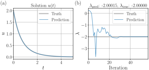
where λ and µ are two parameters. Here we set λ " ´2.0 and µ " 2.0. The analytic solution to (26) is
There is only one initial point so NB " 1, and NL " 50 in (7) in the forward problem. In the inverse problem, we assume that λ is unknown and set NB`NL " 50. In both cases Ntest is equal to 2000. Table 2 provides the average results of three independent runs. KP-PINNs and RKHS-PINNs yield similar results due to the same loss function form, but differ in the computation of K´1 , leading to the run-time gap observed in Table 6, where KP-PINNs demonstrate significantly faster computation across all four equations. The SobolevPINNs algorithm uses automatic differentiation to compute first- and higher-order derivatives, leading to error accumulation and difficulty in obtaining accurate results.
5.2 Helmholtz Equation
The Helmholtz equation is a second-order elliptic PDE commonly encountered in electromagnetism that describes the spatial behavior of electromagnetic wave propagation. It is defined by
| Algorithm (-PINNs) | Forward | SE | Inverse | SE | Inv λp-2.0q |
|---|---|---|---|---|---|
| KP (ν " 12 ) | 2.23e-04 | 4.90e-05 | 3.95e-04 | 1.37e-04 | -1.99983 |
| KP (ν " 32 ) | 5.57e-04 | 3.83e-04 | 5.62e-04 | 2.79e-04 | -2.00015 |
| KP (ν " 52 ) | 1.55e-04 | 6.64e-05 | 3.25e-04 | 1.43e-04 | -1.99991 |
| L2 | 3.31e-04 | 4.13e-05 | 3.32e-04 | 1.34e-04 | -1.99995 |
| RKHS (ν " 12 ) | 2.90e-04 | 8.19e-05 | 3.93e-04 | 1.35e-04 | -1.99983 |
| RKHS (ν " 32 ) | 5.83e-04 | 3.70e-04 | 3.75e-04 | 3.25e-04 | -1.99984 |
| RKHS (ν " 52 ) | 1.29e-04 | 5.09e-05 | 3.24e-04 | 1.41e-04 | -1.99991 |
| Sobolev (ν " 1) | 5.62e-02 | 4.57e-02 | 4.38e-01 | 8.75e-03 | -1.05663 |
| Sobolev (ν " 2) | 3.58e-01 | 1.38e-02 | 4.12e-01 | 1.94e-02 | -1.29371 |
| Sobolev (ν " 3) | 3.56e-01 | 8.57e-03 | 4.29e-01 | 2.60e-02 | -1.64380 |
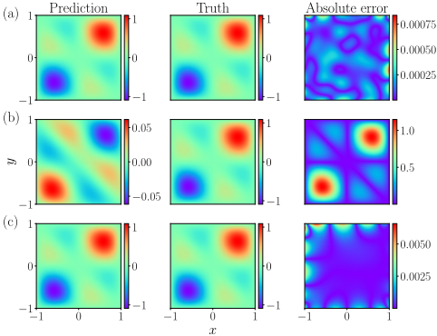
where ∆u " B2 u Bx2 ` B2 u By2 , k is the wave number, p is the source term (excitation term) [Li et al., 2022] defined by ppx, yq " px ` yq sinpπxq sinpπyq ´ 2π2 px ` yq sinpπxq sinpπyq ` 2π cospπyq sinpπxq ` 2π cospπxq sinpπyq. Here, we set k " 1.0. The analytic solution for k " 1.0 [Jagtap et al., 2020] is
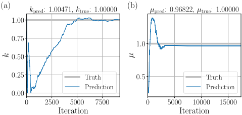
In this experiment, NB " 100 and NL " 100 ˆ 100 in (7). For the inverse problem, parameter k is unknown and NB`NL " 30ˆ30 in (7). In both casesNtest is equal to 500ˆ 600. Table 3 gives the average results of five times. It can be seen that the first three algorithms can get the solutions well. For inverse problems, only KP-PINNs (ν " 1 2 ) and RKHSPINNs (ν " 12 ) can predict the k relatively correctly, while the L2-PINNs fails to work. Figure 2 (b), Figure 2 (c) and Figure 3 (a) show the inverse problem results of L2-PINNs and KP-PINNs (ν " 12 ). The parameter ν determines the degree of smoothness for the kernel function, and a smaller value of ν is suitable for less smooth conditions. It can be seen that a smaller ν (such as ν " 12 ) can get better results.
| Algorithm (-PINNs) | Forward | Standard | Inverse | Standard | Inv k (1.0) |
|---|---|---|---|---|---|
| KP (ν " 12 ) | 1.13e-03 | 1.97e-04 | 4.88e-03 | 1.10e-03 | 0.98262 |
| KP (ν " 32 ) | 9.13e-04 | 1.91e-04 | 1.26e-02 | 7.35e-03 | 0.83391 |
| KP (ν " 52 ) | 1.15e-03 | 1.91e-04 | 2.75e-02 | 7.20e-03 | 0.51944 |
| L2 | 2.99e-03 | 3.06e-04 | 2.36e-01 | 2.05e-01 | 4.37582 |
| RKHS (ν " 12 ) | 2.10e-03 | 9.61e-04 | 3.37e-03 | 6.26e-04 | 0.99927 |
| RKHS (ν " 32 ) | 1.02e-03 | 1.23e-04 | 1.68e-02 | 7.58e-03 | 0.77236 |
| RKHS (ν " 52 ) | 1.10e-03 | 1.65e-04 | 1.88e-02 | 7.34e-03 | 0.69293 |
| Sobolev (ν " 1) | 1.79e+00 | 1.01e+00 | 7.41e-01 | 4.82e-01 | 0.00475 |
| Sobolev (ν " 2) | 8.95e-01 | 2.09e-02 | 3.85e-01 | 1.64e-02 | 0.00221 |
| Sobolev (ν " 3) | 1.31e+01 | 8.85e+00 | 8.20e-01 | 1.00e-01 | 0.01159 |
5.3 Linear Quadratic Gaussian (LQG) Equation
One application of the HJB equation is LQG control problem. The form of LQG [Han et al., 2018] in d dimensions are
with the solution
where gpxq " ln ´ 1`||x||2 2 ¯ is the terminal cost function.
We set d " 2, µ " 1.0, T " 1.0,NB " 2000 and NL " 30 ˆ 20 ˆ 10 in (7) in the forward problem. For the inverse problem, µ is unknown and NB `NL " 10ˆ10ˆ10. In both cases, Ntest is equal to 100 ˆ 80 ˆ 50. Table 4 gives the average results of three times experiments. For the inverse problem, KP-PINNs with ν " 12 can obtain the closest estimation among all algorithms. Figure 3 (b) gives a one-case inverse problem results of KP-PINNs (ν " 12 ).
5.4 Navier-Stokes (NS) Equation
The widely-used NS equations are fundamental PDEs that describe the motion of viscous and incompressible fluids. In this experiment, the two-dimensional incompressible NS equations are considered to model the evolution of fluid flow. The governing equation for the vorticity ωpt, x, yq is
| Algorithm (-PINNs) | Forward | Standard | Inverse | Standard | Inv µ (1.0) |
|---|---|---|---|---|---|
| KP (ν " 12 ) | 6.70e-02 | 2.43e-02 | 6.90e-03 | 8.84e-04 | 0.93244 |
| KP (ν " 32 ) | 2.26e-01 | 8.56e-02 | 1.81e-02 | 1.45e-03 | 1.26715 |
| KP (ν " 52 ) | 3.46e-01 | 1.89e-02 | 1.88e-02 | 2.29e-03 | 1.27243 |
| L2 | 2.39e-01 | 9.80e-02 | 1.77e-02 | 1.36e-03 | 1.20942 |
| RKHS (ν " 12 ) | 1.71e-01 | 6.90e-02 | 8.25e-03 | 2.28e-03 | 0.93072 |
| RKHS (ν " 32 ) | 3.21e-01 | 8.89e-03 | 1.88e-02 | 2.17e-03 | 1.27210 |
| RKHS (ν " 52 ) | 3.39e-01 | 5.54e-03 | 1.89e-02 | 1.94e-03 | 1.25183 |
| Sobolev (ν " 1) | 1.42e+00 | 3.43e-02 | 6.05e-01 | 9.27e-02 | -1.21866 |
| Sobolev (ν " 2) | 1.43e+00 | 3.37e-04 | 7.12e-03 | 9.39e-05 | -129.13841 |
| Sobolev (ν " 3) | 7.05e-02 | 3.33e-02 | 1.51e-02 | 3.12e-03 | 1.16909 |
| Algorithm (-PINNs) | Forward | Standard | Inverse | Standard | Inv µ (0.01) |
|---|---|---|---|---|---|
| KP (ν " 1 2 ) | 1.66e-01 | 9.90e-03 | 3.61e-02 | 1.75e-02 | 0.01176 |
| L2 | 3.97e-01 | 1.18e-01 | 1.40e-01 | 5.46e-02 | 0.01233 |
| RKHS (ν " 1 2 ) | 1.73e-01 | 6.66e-03 | 4.87e-02 | 1.07e-02 | 0.01201 |
| Algorithm (-PINNs) | Stiff | Helmholtz | LQG | NS |
|---|---|---|---|---|
| KP (ν " 1 2 ) | 0.2971s | 5.3152s | 90.7398s | 26.9730s |
| RKHS (ν " 1 2 ) | 2.6984s | 42.1662s | 431.0374s | 56.9642s |
Table 6: Time of computing K´1 (ν " 12 as example). NB `NL " 2000 for Stiff equation. NB ` NL " 200 ˆ 300 for Helmholtz equation. NB`NL " 50ˆ50ˆ40 for LQG equation. NB`NL " 60 ˆ 40 ˆ 20 for NS equation.
where µ is the viscosity coefficient. In our experiment, we set µ " 0.01, T " 1.9, xstart " 1.0, xend " 8.0, ystart " ´2.0 and yend " 2.0. The initial condition is the situation of t " 0. The boundary conditions are the situation of x " xstart, x " xend, y " ystart and y " yend. The vorticity is defined in terms of the stream function ψpt, x, yq by the Poisson equation ω " ´pψxx ` ψyyq. The velocity components pu, vq can be recovered from the stream function as u " ψy, v " ´ψx. The two components of the velocity field data upt, x, yq and vpt, x, yq are obtained from [Raissi et al., 2019], where the numerical solution is performed. We approximate the stream function ψ using a neural network. The velocity field and vorticity can be derived by automatic differentiation.
We set NB " 5000 and NL " 30ˆ20ˆ10 in (7). For the inverse problem, µ is unknown and NB `NL " 10ˆ10ˆ10. In both cases, Ntest " 98 ˆ 48 ˆ 20. Table 5 shows the averaged results over three independent runs. It can be seen that KP-PINNs, L2-PINNs and RKHS-PINNs can solve the equation in general. Among them, KP-PINNs and RKHS-PINNs consistently demonstrate superior performance in terms of both accuracy and robustness. For the inverse problem, KPPINNs(ν " 1 2 ) can obtain the closest estimation.
6 Conclusion
This work proposes KP-PINNs, an efficient method for solving differential equations, with stability guarantees for second-order linear elliptic and HJB equations under certain conditions. Numerical experiments demonstrate that KPPINNs outperform L2-PINNs and Sobolev-PINNs for both forward and inverse problems, significantly accelerating the computation of the inverse of kernel matrix K through the KP technique. Future directions include extending KP-PINNs to handle sparse or irregular data, optimizing neural network architecture, and refining kernel selection in the loss function to improve accuracy and robustness. These advancements aim to enhance KP-PINNs' versatility in solving complex differential equations.
Acknowledgments
This research is supported by Guangdong Provincial Fund - Special Innovation Project (2024KTSCX038).
@inproceedings{ijcai2025p879,
  title     = {KP-PINNs: Kernel Packet Accelerated Physics Informed Neural Networks},
  author    = {Yang, Siyuan and Song, Cheng and Lai, Zhilu and Wang, Wenjia},
  booktitle = {Proceedings of the Thirty-Fourth International Joint Conference on
               Artificial Intelligence, {IJCAI-25}},
  publisher = {International Joint Conferences on Artificial Intelligence Organization},
  editor    = {James Kwok},
  pages     = {7904--7912},
  year      = {2025},
  month     = {8},
  note      = {Main Track},
  doi       = {10.24963/ijcai.2025/879},
  url       = {https://doi.org/10.24963/ijcai.2025/879},
}
TY - CPAPER TI - KP-PINNs: Kernel Packet Accelerated Physics Informed Neural Networks AU - Yang, Siyuan AU - Song, Cheng AU - Lai, Zhilu AU - Wang, Wenjia T2 - Proceedings of the Thirty-Fourth International Joint Conference on Artificial Intelligence, IJCAI-25 PB - International Joint Conferences on Artificial Intelligence Organization PY - 2025 SP - 7904 EP - 7912 DO - 10.24963/ijcai.2025/879 UR - https://doi.org/10.24963/ijcai.2025/879 ER -Copied
Machine-readable versions of this paper, for tools and AI agents:





