
X-KAN: Optimizing Local Kolmogorov-Arnold Networks via Evolutionary Rule-Based Machine Learning
Proceedings of the Thirty-Fourth International Joint Conference on Artificial Intelligence. Main Track. Pages 8930-8938.
https://doi.org/10.24963/ijcai.2025/993
Keywords
- Machine Learning: ML: Evolutionary learning
- Search: S: Search and machine learning
- Search: S: Evolutionary computation
Abstract
Function approximation is a critical task in various fields. However, existing neural network approaches struggle with locally complex or discontinuous functions due to their reliance on a single global model covering the entire problem space. We propose X-KAN, a novel method that optimizes multiple local Kolmogorov-Arnold Networks (KANs) through an evolutionary rule-based machine learning framework called XCSF. X-KAN combines KAN's high expressiveness with XCSF's adaptive partitioning capability by implementing local KAN models as rule consequents and defining local regions via rule antecedents. Our experimental results on artificial test functions and real-world datasets demonstrate that X-KAN significantly outperforms conventional methods, including XCSF, Multi-Layer Perceptron, and KAN, in terms of approximation accuracy. Notably, X-KAN effectively handles functions with locally complex or discontinuous structures that are challenging for conventional KAN, using a compact set of rules (average 7.2 rules). These results validate the effectiveness of using KAN as a local model in XCSF, which evaluates the rule fitness based on both accuracy and generality. Our X-KAN implementation and an extended version of this paper, including appendices, are available at https://doi.org/10.48550/arXiv.2505.14273.
- [Arnol'd, 1957] Vladimir Igorevich Arnol'd. On functions of three variables. In Doklady Akademii Nauk, volume 114, pages 679-681. Russian Academy of Sciences, 1957.
- [Bao et al., 2022] Dan Bao, Xiaoling Liang, Shuzhi Sam Ge, and Baolin Hou. Adaptive neural trajectory tracking con- trol for n-dof robotic manipulators with state constraints. IEEE Transactions on Industrial Informatics, 19(7):8039- 8048, 2022.
- [Bezanson et al., 2017] Jeff Bezanson, Alan Edelman, Ste- fan Karpinski, and Viral B Shah. Julia: A fresh approach to numerical computing. SIAM review, 59(1):65-98, 2017.
- [Bull and O'Hara, 2002] Larry Bull and Toby O'Hara. Accuracy-based neuro and neuro-fuzzy classifier systems. In Proceedings of the 4th Annual Conference on Genetic and Evolutionary Computation, pages 905-911, 2002.
- [Butz et al., 2008] Martin V Butz, Pier Luca Lanzi, and Stewart W Wilson. Function approximation with XCS: Hyperellipsoidal conditions, recursive least squares, and compaction. IEEE Transactions on Evolutionary Compu- tation, 12(3):355-376, 2008.
- [Chen et al., 2024] Xia Chen, Guoquan Lv, Xinwei Zhuang, Carlos Duarte, Stefano Schiavon, and Philipp Geyer. In- tegrating symbolic neural networks with building physics: A study and proposal. arXiv preprint arXiv:2411.00800, 2024.
- [Cheon, 2024] Minjong Cheon. Kolmogorov-arnold net- work for satellite image classification in remote sensing. arXiv preprint arXiv:2406.00600, 2024.
- [Cybenko, 1989] George Cybenko. Approximation by su- perpositions of a sigmoidal function. Mathematics of con- trol, signals and systems, 2(4):303-314, 1989.
- [De Boor, 1978] Carl De Boor. A practical guide to splines. Springer-Verlag google schola, 2:4135-4195, 1978.
- [De Franceschi et al., 2024] Gianluca De Franceschi, Inês W Sampaio, Stefan Borgwardt, Joseph Kambeitz, Lana Kambeitz-Ilankovic, Eva Meisenzahl, Raimo KR Salokangas, Rachel Upthegrove, Stephen J Wood, Niko- laos Koutsouleris, et al. Ensemble-kan: Leveraging kolmogorov arnold networks to discriminate individuals with psychiatric disorders from controls. In International Workshop on Applications of Medical AI, pages 186-197.
- [de Zarzà et al., 2023] I de Zarzà, J de Curtò, and Carlos T Calafate. Optimizing neural networks for imbalanced data. Electronics, 12(12):2674, 2023.
- [Elfwing et al., 2018] Stefan Elfwing, Eiji Uchibe, and Kenji Doya. Sigmoid-weighted linear units for neural network function approximation in reinforcement learning. Neural networks, 107:3-11, 2018.
- [Gandomi and Alavi, 2011] Amir Hossein Gandomi and Amir Hossein Alavi. Multi-stage genetic programming: a new strategy to nonlinear system modeling. Information Sciences, 181(23):5227-5239, 2011.
- [Hansmeier et al., 2020] Tim Hansmeier, Paul Kaufmann, and Marco Platzner. An adaption mechanism for the er- ror threshold of XCSF. In Proceedings of the 2020 Ge- netic and Evolutionary Computation Conference Compan- ion, pages 1756-1764, 2020.
- [Hecht-Nielsen, 1987] Robert Hecht-Nielsen. Kolmogorov's mapping neural network existence theorem. In Proceed- ings of the international conference on Neural Networks, volume 3, pages 11-14. IEEE press, 1987.
- [Heider et al., 2023] Michael Heider, Helena Stegherr, Ro- man Sraj, David Pätzel, Jonathan Wurth, and Jörg Hähner. Suprb in the context of rule-based machine learning meth- ods: A comparative study. Applied Soft Computing, 147:110706, 2023.
- [Hornik et al., 1989] Kurt Hornik, Maxwell Stinchcombe, and Halbert White. Multilayer feedforward networks are universal approximators. Neural networks, 2(5):359-366, 1989.
- [Howard et al., 2024] Amanda A Howard, Bruno Jacob, Sarah H Murphy, Alexander Heinlein, and Panos Stinis. Finite basis kolmogorov-arnold networks: domain decom- position for data-driven and physics-informed problems. arXiv preprint arXiv:2406.19662, 2024.
- [Ishibuchi et al., 1999] Hisao Ishibuchi, Tomoharu Nakashima, and Tadahiko Murata. Performance eval- uation of fuzzy classifier systems for multidimensional pattern classification problems. IEEE Transactions on Systems, Man, and Cybernetics, Part B (Cybernetics), 29(5):601-618, 1999.
- [Kolmogorov, 1961] Andreȋ Nikolaevich Kolmogorov. On the representation of continuous functions of several vari- ables by superpositions of continuous functions of a smaller number of variables. American Mathematical So- ciety, 1961.
- [Lanzi and Loiacono, 2006] Pier Luca Lanzi and Daniele Loiacono. XCSF with neural prediction. In 2006 IEEE international conference on Evolutionary Computation, pages 2270-2276. IEEE, 2006.
- [Lanzi and Wilson, 2006] Pier Luca Lanzi and Stewart W Wilson. Using convex hulls to represent classifier con- ditions. In Proceedings of the 8th annual conference on Genetic and evolutionary computation, pages 1481-1488, 2006.
- [Lanzi et al., 2005] Pier Luca Lanzi, Daniele Loiacono, Stewart W Wilson, and David E Goldberg. Extending XCSF beyond linear approximation. In Proceedings of the 7th annual conference on Genetic and evolutionary com- putation, pages 1827-1834, 2005.
- [Lanzi et al., 2007] Pier Luca Lanzi, Daniele Loiacono, Stewart W Wilson, and David E Goldberg. Generalization in the XCSF classifier system: Analysis, improvement, and extension. Evolutionary Computation, 15(2):133-168, 2007.
- [Liu et al., 2024] Ziming Liu, Yixuan Wang, Sachin Vaidya, Fabian Ruehle, James Halverson, Marin Soljačić, Thomas Y Hou, and Max Tegmark. KAN: Kolmogorov- arnold networks. arXiv preprint arXiv:2404.19756, 2024.
- [Livieris, 2024] Ioannis E Livieris. C-kan: A new approach for integrating convolutional layers with kolmogorov- arnold networks for time-series forecasting. Mathematics, 12(19):3022, 2024.
- [Loiacono et al., 2007] Daniele Loiacono, Andrea Marelli, and Pier Luca Lanzi. Support vector regression for clas- sifier prediction. In Proceedings of the 9th annual con- ference on Genetic and evolutionary computation, pages 1806-1813, 2007.
- [Mirza et al., 2024] Fuat Kaan Mirza, Tunc ¸er Baykas ¸, Mustafa Hekimoglu, Önder Pekcan, and Gönül Pac ¸acı Tunc ¸ay. Decoding compositional complexity: Identify- ing composers using a model fusion-based approach with nonlinear signal processing and chaotic dynamics. Chaos, Solitons & Fractals, 187:115450, 2024.
- [Mohan et al., 2024] Karthik Mohan, Hanxiao Wang, and Xiatian Zhu. Kans for computer vision: An experimen- tal study. arXiv preprint arXiv:2411.18224, 2024.
- [Narayanan et al., 2021] Deepak Narayanan, Mohammad Shoeybi, Jared Casper, Patrick LeGresley, Mostofa Pat- wary, Vijay Korthikanti, Dmitri Vainbrand, Prethvi Kashinkunti, Julie Bernauer, Bryan Catanzaro, et al. Effi- cient large-scale language model training on gpu clusters using megatron-lm. In Proceedings of the International Conference for High Performance Computing, Network- ing, Storage and Analysis, pages 1-15, 2021.
- [Orriols-Puig et al., 2008] Albert Orriols-Puig, Jorge Casil- las, and Ester Bernadó-Mansilla. Fuzzy-UCS: a michigan- style learning fuzzy-classifier system for supervised learn- ing. IEEE Transactions on Evolutionary Computation, 13(2):260-283, 2008.
- [Pätzel and Hähner, 2022] David Pätzel and Jörg Hähner. The bayesian learning classifier system: implementation, replicability, comparison with XCSF. In Proceedings of the Genetic and Evolutionary Computation Conference, pages 413-421, 2022.
- [Preen et al., 2021] Richard J. Preen, Stewart W. Wilson, and Larry Bull. Autoencoding with a classifier system. IEEE Transactions on Evolutionary Computation, 25(6):1079- 1090, 2021.
- [Qiu et al., 2024] Ruichen Qiu, Yibo Miao, Shiwen Wang, Lijia Yu, Yifan Zhu, and Xiao-Shan Gao. Pow- erMLP: An efficient version of KAN. arXiv preprint arXiv:2412.13571, 2024.
- [Shiraishi et al., 2022] Hiroki Shiraishi, Yohei Hayamizu, Hiroyuki Sato, and Keiki Takadama. Beta distribution based XCS classifier system. In 2022 IEEE Congress on Evolutionary Computation (CEC), pages 1-8. IEEE, 2022.
- [Shoji et al., 2023] Takaharu Shoji, Masaki Kuriyama, and Masaya Nakata. Piecewise symbolic regression by evo- lutionary rule-based learning with genetic programming. IPSJ Transactions on Mathematical Modeling and its Ap- plications (TOM), 16(2):36-49, 2023.
- [Siddique et al., 2024] Abubakar Siddique, Michael Heider, Muhammad Iqbal, and Hiroki Shiraishi. A survey on learning classifier systems from 2022 to 2024. In Proceed- ings of the Genetic and Evolutionary Computation Confer- ence Companion, pages 1797-1806, 2024.
- [Somvanshi et al., 2024] Shriyank Somvanshi, Syed Aaqib Javed, Md Monzurul Islam, Diwas Pandit, and Subasish Das. A survey on kolmogorov-arnold network. arXiv preprint arXiv:2411.06078, 2024.
- [Stein et al., 2018] Anthony Stein, Simon Menssen, and Jörg Hähner. What about interpolation? a radial basis function approach to classifier prediction modeling in XCSF. In Proceedings of the Genetic and Evolutionary Computation Conference, pages 537-544, 2018.
- [Stone and Bull, 2003] Christopher Stone and Larry Bull. For real! XCS with continuous-valued inputs. Evolution- ary Computation, 11(3):299-336, 2003.
- [Tang et al., 2019] Huimin Tang, Peiwu Dong, and Yong Shi. A new approach of integrating piecewise linear repre- sentation and weighted support vector machine for fore- casting stock turning points. Applied Soft Computing, 78:685-696, 2019.
- [Urbanowicz and Browne, 2017] Ryan J Urbanowicz and Will N Browne. Introduction to learning classifier sys- tems. Springer, 2017.
- [Widrow and Hoff, 1960] Bernard Widrow and Marcian E Hoff. Adaptive switching circuits. Technical report, Stan- ford Univ Ca Stanford Electronics Labs, 1960.
- [Wilson, 1998] Stewart W Wilson. Generalization in the XCS classifier system. Proc. Genetic Programming, 1998.
- [Wilson, 2002] Stewart W Wilson. Classifiers that approxi- mate functions. Natural Computing, 1(2):211-234, 2002.
- [Wilson, 2006] Stewart W Wilson. Classifier conditions using gene expression programming. In International Workshop on Learning Classifier Systems, pages 206-217. Springer, 2006.
- [Xu et al., 2024] Kunpeng Xu, Lifei Chen, and Shengrui Wang. Kolmogorov-arnold networks for time series: Bridging predictive power and interpretability. arXiv preprint arXiv:2406.02496, 2024.
- [Yu et al., 2024] Runpeng Yu, Weihao Yu, and Xinchao Wang. KAN or MLP: A fairer comparison. arXiv preprint arXiv:2407.16674, 2024.
- [Zeydan et al., 2025] Engin Zeydan, Cristian J Vaca-Rubio, Luis Blanco, Roberto Pereira, Marius Caus, and Abdul- lah Aydeger. F-kans: Federated kolmogorov-arnold net- works. In 2025 IEEE 22nd Consumer Communications & Networking Conference (CCNC), pages 1-6. IEEE, 2025.
References were extracted automatically from the PDF and may contain errors.
Full text extracted automatically from the PDF; figures, tables and equations may differ. The PDF is the version of record.
1 Introduction
Function approximation is a crucial task in various industrial fields, including control system design and signal processing [Bao et al., 2022; Mirza et al., 2024]. The function approximation problem addressed in this paper aims to discover the most suitable approximation function for given data points, and can be formalized as follows:
∗Corresponding authors.
where D is a training dataset, n is the input dimensionality, M is the total number of data points in D, ˆ f : Rn → R is the approximation function, and L : R × R → R+0 is the loss function. The difficulty of this problem becomes particularly evident when dealing with functions that exhibit strong nonlinearity or data with complex structures.
Multi-Layer Perceptrons (MLPs) [Cybenko, 1989], a type of neural networks, have been widely studied as a representative approach to function approximation. MLPs have been proven to approximate any continuous function with arbitrary precision using fixed nonlinear activation functions [Hornik et al., 1989]. Their effectiveness has been demonstrated in various fields, including modeling complex physical phenomena, image recognition, and recent large-scale language models [de Zarz`a et al., 2023; Preen et al., 2021; Narayanan et al., 2021]. However, their reliance on fixed nonlinear activation functions often requires large numbers of parameters to approximate complex functions effectively, which leads to inefficiencies [Mohan et al., 2024].
Kolmogorov-Arnold Networks (KANs) [Liu et al., 2024], inspired by the Kolmogorov-Arnold representation theorem [Kolmogorov, 1961; Arnol'd, 1957], have recently been proposed as a promising alternative. Unlike MLPs, KANs utilize spline-based learnable activation functions, enabling them to achieve higher parameter efficiency and scalability for irregular functions. KANs have shown superior performance in diverse applications such as image processing, time series prediction, and natural language processing [Cheon, 2024; Somvanshi et al., 2024; Livieris, 2024]. Given their early successes, KANs are expected to attract increasing attention for a wide range of applications [Xu et al., 2024].
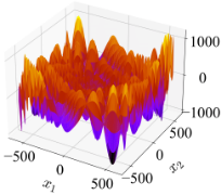
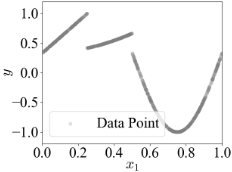
Despite their advantages, KANs share a common limitation with MLPs: they rely on a single global model to approximate the entire problem space. This approach implicitly assumes that all data points follow the same underlying function. However, in reality, there are problems that cannot be adequately solved by a single global model. For instance, functions with local complexities (e.g., Fig 2) or discontinuities (e.g., Fig. 3a) pose significant challenges. Such problems are frequently encountered in real-world applications, including stock price prediction [Tang et al., 2019] and multistage control system analysis [Gandomi and Alavi, 2011].
To address these concerns, the X Classifier System for Function Approximation (XCSF) [Wilson, 2002], a widely studied evolutionary rule-based machine learning algorithm [Siddique et al., 2024], may offer a promising solution. XCSF employs a divide-and-conquer approach that adaptively partitions the input space and assigns a distinct approximation model to each local region. XCSF enables localized modeling of complex functions, potentially complementing KAN's limitations in handling locally complex structures.
This paper proposes X-KAN, a function approximation method that simultaneously utilizes KAN's high representational power and XCSF's adaptive partitioning capability. XKAN represents the entire input space using multiple local KANmodels. Specifically, it defines a local region in the rule antecedent (i.e., IF part) and implements a KAN model in the rule consequent (i.e., THEN part), expressing local KAN models as rules. These IF-THEN rules are evolutionarily optimized by the XCSF framework. X-KAN is expected to improve approximation accuracy for functions with inherent local nonlinearities or discontinuities compared to a conventional single global KAN model.
The contributions of this paper are as follows:
- We integrate KANs into evolutionary rule-based machine learning for the first time by introducing KANs into the XCSF framework. The effectiveness of this idea is demonstrated through artificial and real-world function approximation problems.
- We propose the first algorithm to automatically optimize multiple local KAN models. This results in a significant reduction in testing approximation error compared to conventional single global KAN models. We also explain that this effectiveness is due to XCSF's fundamental principle of assigning high fitness to local models (i.e., rules) with high generality and accuracy.
Note that recent studies have explored combining multiple KAN models for improved accuracy in various settings. For instance, Ensemble-KAN [De Franceschi et al., 2024] constructs several KANs using different subsets of input features and aggregates their outputs. Federated-KANs [Zeydan et al., 2025] focus on distributed training across federated clients. Unlike these approaches, X-KAN uniquely integrates adaptive input space partitioning with local KAN optimization. Moreover, in contrast to approaches that predefine domain decompositions [Howard et al., 2024], X-KAN simultaneously learns both the optimal partitioning of the input space and the parameters of local KAN models. This dual optimization enables X-KAN to automatically discover and model complex local structures and discontinuities in data, setting it apart from existing methods.
The remainder of this paper is organized as follows. Section 2 provides background on MLPs, KANs, and XCSF. Section 3 presents our proposed algorithm, X-KAN. Section 4 reports and discusses experimental results. Section 5 presents further studies. Finally, Section 6 concludes the paper.
2 Background
2.1 MLPs and KANs
Multi-Layer Perceptrons (MLPs)
Multi-Layer Perceptrons (MLPs) are feedforward neural network architectures widely studied for function approximation problems. For a three-layer MLP with n inputs, H hidden nodes, and a single output, the forward computation can be expressed in matrix form as:
where W(1) ∈ RH×n is the weight matrix between the input and hidden layers, w(2) ∈ R1×H is the weight vector between the hidden and output layers, b(1) ∈ RH and b(2) ∈ R are bias terms, and σ is a fixed nonlinear activation function, e.g., Sigmoid-weighted Linear Unit (SiLU) [Elfwing et al., 2018]. The MLP architecture is illustrated in Appendix A. According to [Yu et al., 2024], the total number of parameters for this three-layer MLP, denoted as NMLP, is:
Based on the Universal Approximation Theorem (UAT) [Hornik et al., 1989], MLPs with a single hidden layer can approximate any continuous function on compact subsets of Rn to arbitrary precision, as detailed in Appendix B. However, MLPs often require a large number of parameters to approximate complex functions [Mohan et al., 2024].
Kolmogorov-Arnold Networks (KANs)
Kolmogorov-Arnold Networks (KANs) are neural networks designed based on the Kolmogorov-Arnold representation theorem (KART). Further details of KART are provided in Appendix C. For a three-layer KAN with n inputs, the matrix representation is:
where:
represents the first layer as a collection of learnable univariate activation functions, and:
represents the second layer as a collection of learnable univariate activation functions. The KAN model expressed in Eq. (5) is mathematically equivalent to the KART formulation, which is presented in Eq. (20) of Appendix C.
Each activation function ϕ(x) is parameterized as:
where SiLU(x) = x/(1+e-x ), spline(x) = ∑G+K i=1 ciBi(x) with B-spline basis functions Bi(x) [De Boor, 1978], and cis, wb, and ws are optimized via backpropagation. The KAN architecture is illustrated in Appendix A. According to [Yu et al., 2024], the total number of parameters for this three-layer KAN, denoted as NKAN, is:
where G is the number of B-spline grids and K is the B-spline degree.
Unlike MLPs, which use a fixed activation function at each node, KANs implement a learnable activation function on each edge between nodes. This design allows KANs to capture complex nonlinear relations more efficiently than MLPs. By leveraging KART, a KAN model handles the learning of a high-dimensional function as the learning of multiple univariate functions. This enables KANs to achieve higher parameter efficiency compared to MLPs, especially for problems involving complex data [Liu et al., 2024]. However, it is important to note that KART guarantees representations only for continuous functions. As a result, KAN may struggle to approximate discontinuous functions effectively.
2.2 XCSF
Overview
Wilson's X Classifier System for Function Approximation (XCSF) [2002] is a rule-based piecewise function approximation method that implements linear regression models in rule consequents and hyperrectangular partitions in rule antecedents. 1 XCSF combines evolutionary algorithms (EA) and stochastic gradient descent to generate general linear models with wide matching ranges in rule antecedents.
The key characteristics of XCSF are twofold. First, XCSF employs a subsumption operator [Wilson, 1998] that aggregates multiple similar rules into a single, more general rule. Second, XCSF evaluates rule fitness based on both the number of aggregated rules and approximation error, optimizing the rule structure based on this fitness. Based on these two characteristics, XCSF promotes the acquisition of general linear models and realizes its fundamental principle of efficiently approximating data points with as few linear models as possible. Appendix D provides further details of XCSF.
Extensions
Since Wilson [2002] proposed XCSF, various extensions have been developed. For rule consequents, polynomial models [Lanzi et al., 2005], MLPs [Lanzi and Loiacono, 2006], support vector machines [Loiacono et al., 2007], and radial basis functions [Stein et al., 2018] have been proposed to enable the approximation of more complex nonlinear functions. For rule antecedents, hyperellipsoids [Butz et al., 2008], curved polytopes [Shiraishi et al., 2022], convex hulls [Lanzi and Wilson, 2006], gene expression programming [Wilson, 2006], and MLPs [Bull and O'Hara, 2002] have been introduced to achieve more flexible input space partitions. These extensions contribute to improving XCSF's approximation accuracy. Recently, XCSF was first applied to unsupervised autoencoding tasks by using MLPs as rule antecedents and autoencoders as rule consequents [Preen et al., 2021].
These extensions show XCSF's extensibility and validate XCSF's core principle of decomposing complex input spaces through rules. Our proposed integration of KAN into XCSF's rule consequents leverages KAN's universal approximation capabilities [Hecht-Nielsen, 1987], guaranteed by KART, to achieve superior approximation accuracy compared to traditional XCSF approaches.
1 XCSF is a representative method of Learning Classifier Systems (LCS) [Urbanowicz and Browne, 2017], a family of rule-based machine learning algorithms. Historically, rules in LCS, including XCSF, are called classifiers even when they work as regression models rather than classification models [P¨atzel and H¨ahner, 2022]. To avoid this ambiguity in terminology, we use the term rule.
3 X-KAN
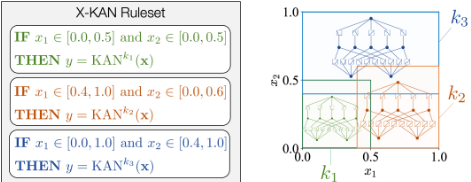
We introduce X-KAN, a function approximation method that optimizes multiple local KAN models. Fig. 1 schematically illustrates X-KAN. X-KAN leverages the strengths of KAN's high expressiveness and XCSF's adaptive partitioning to address the limitations of conventional global function approximators. X-KAN has three key characteristics:
- Local KAN Rules. Each rule in X-KAN consists of an antecedent defined as an n-dimensional hyperrectangle and a consequent implemented as a single KAN model. This structure allows each rule to play a role as a local function approximator, activating only for the local region specified by its antecedent.
- Dual Optimization. Utilizing the XCSF framework, XKAN constructs general and accurate local KAN models with wide matching ranges. The rule antecedents are optimized through the EA, while the rule consequents (local KAN models) are optimized via backpropagation. This dual optimization enables X-KAN to adaptively place optimal local KANmodels in each local region.
- Divide-and-Conquer. Unlike KAN that operates as a single global function approximator, X-KAN functions as a divide-and-conquer algorithm by integrating multiple local KAN models having distinct activation functions.
3.1 Rule Representation
An n-dimensional rule k in X-KAN is expressed as:
where:
- Ak = (lk , uk ) = (lk i , uki )ni=1 is the antecedent as a hyperrectangle with bounds lk , uk ∈ [0, 1]n and lk i < uki for all i [Stone and Bull, 2003];
- KANk (·) is the consequent KANmodel of rule k;
- F k ∈ (0, 1] is the fitness value that evaluates both accuracy and generality of rule k.
Algorithm 1 X-KAN training mode
Input: the training dataset D = (X , Y) = {(x, y) ∈ [0, 1]n × R}; Output: the compacted ruleset PC; 1: Initialize time t as t ← 0; 2: Initialize ruleset P as P ← ∅; 3: while t < the maximum number of iterations do 4: Observe a data point (x, y) ∈ D; 5: Create match setM⊆ P as in Eq. (11); 6: if M = ∅ then 7: Do covering to generate a new rule kc; 8: Insert kc to P andM; 9: end if 10: Update F k for ∀k ∈Mas in Eq. (16); 11: if t - ∑k∈M numk · tsk /∑k∈M numk > θEA then 12: Update time stamp tsk for ∀k ∈Mas tsk ← t; 13: Run EA on M; 14: Do subsumption; 15: end if 16: Update time t as t ← t +1; 17: end while 18: Create compacted ruleset PC ⊆ P as in Eq. (17); 19: return PCEach rule k maintains four key parameters: (i) Error ϵk ∈ R+0 , representing absolute approximation error of the consequent KAN model; (ii) Accuracy κk ∈ (0, 1], calculated based on the error; (iii) Generality numk ∈ N0, indicating the number of aggregated rules; and (iv) Time stamp tsk ∈ N0, representing the last time the rule was a candidate for the EA.
Ak , KANk (·), ϵk , and κk are uniquely determined and fixed when a rule is generated, either during the covering operation or by the EA. In contrast, F k , numk , and tsk are dynamically updated throughout the training process.
3.2 Algorithm
X-KAN operates in two distinct modes: training mode and testing mode. In training mode, X-KAN explores the search space to identify an accurate and general ruleset using a training dataset. Afterward, it performs rule compaction to produce a compact ruleset, denoted as PC. In testing mode, PC is used to predict the output for testing data points.
Training Mode
Algorithm 1 presents our algorithm for X-KAN training. Match Set Formation and Covering Operation. Let P be the current population of rules. At time t, a data point (x, y) is randomly sampled from the training dataset D (line 4). Subsequently, a match set M is formed as (line 5):
If M = ∅, a new rule kc satisfying x ∈ Akc is generated and inserted into both P and M (lines 6-9). This operation is referred to as covering [Wilson, 2002]. Specifically, using hyperparameters r0 ∈ (0, 1] and P# ∈ [0, 1], the antecedent of kc, Akc = (lkc , ukc ), is determined as:
where U(0, r0] represents a random number uniformly sampled from the range (0, r0]. Eq. (12) ensures that the range for xi is set to Don't Care with probability P#, while otherwise it is set to a region encompassing xi, based on the hyperparameter r0. Next, the subset of data points within the range of kc, denoted as Dkc , is constructed as:
Using this dataset, the local KANmodel of kc, KANkc (·), is trained via backpropagation for a specified number of epochs. The error of kc, ϵkc , is then calculated as:
The error serves as the absolute error for the consequent KAN model of the rule. After that, the accuracy of kc, κkc , is calculated as:
where ϵ0 ∈ R+ is a target error threshold (hyperparameter). Subsequently, key parameters are initialized as follows: F kc = 0.01, numkc = 1, and tskc = 0.
Rule Fitness Update. The fitness of each rule k ∈ M is updated using the Widrow-Hoff learning rule [Widrow and Hoff, 1960] as (line 10):
where β ∈ [0, 1] is the learning rate. As indicated by Eq. (15), X-KAN (based on XCSF) defines a rule k as accurate when its approximation error satisfies ϵk < ϵ0 (i.e., κk = 1). Consequently, the fitness F k , as defined in Eq. (16), assigns higher values to rules with both smaller approximation errors ϵk (i.e., higher accuracy κk ) and larger generality numk .
Application of the EA. After updating the rules, the EA is applied to M (lines 11-15). The EA is triggered when the average time since its last application over all rules inMexceeds a threshold defined by the hyperparameter θEA. In this case, two parent rules kp1 and kp2 are selected fromM using tournament selection with a tournament size of τ. The selected parent rules are duplicated to create two offspring rules ko1 and ko2 . Crossover is applied to their antecedents with a probability of χ. During crossover, for each input dimension i, the lower bound li and the upper bound ui are swapped between the two parents with a probability of 0.5 (i.e., uniform crossover). Subsequently, mutation is applied to each input dimension of the offspring with a probability of µ. In mutation, a random value sampled from a uniform distribution, U[-m0,m0), is added to the bounds lko i and uko i , where ko ∈ {ko1 , ko2 } and m0 ∈ R+ is the maximum mutation magnitude. If the resulting offspring rules ko have antecedents that differ from their parents, their parameters are reinitialized as follows:
- Construct the subset of data points within the antecedent range of ko, denoted as Dko , using Eq. (13).
- Initialize KANko (·) and train it via backpropagation for a specified number of epochs.
- Calculate ϵko and κko using Eqs. (14) and (15).
- Set F ko = 0.1 · f, where f = (F kp1 + F kp2 )/2 if crossover occurs; otherwise, f = F ko . Set numko = 1.
Finally, ko1 and ko2 are added to P if they are not subsumed by their parent rules (described below). If the total generality in P,∑k∈P numk , exceeds the maximum ruleset size N, two rules are deleted, as in [Preen et al., 2021].
Subsumption Operator. X-KAN employs a subsumption operator [Wilson, 1998] to aggregate offspring rules into more general parent rules (line 14). Specifically, for a parent rule kp ∈ {kp1 , kp2 } and an offspring rule ko ∈ {ko1 , ko2 }:
- The parent rule must be more general than the offspring rule (i.e., Akp ⊇ Ako ).
- The parent rule must be accurate (i.e., κkp = 1).
If these conditions are met, the generality of the parent rule is updated as numkp ← numkp +numko and the offspring rule ko is removed fromP.
Rule Compaction. After the training is completed, the rule compaction algorithm [Orriols-Puig et al., 2008] is applied to obtain a compacted ruleset, denoted as PC (line 18). The compacted ruleset is defined as:
For each training data point x, only the rule with the highest fitness (called single winner rule) in its match set M= {k ∈ P | x ∈ Ak } is copied to PC. Appendix H.1 shows that the compaction enables X-KAN to reduce the number of rules by up to 72% while maintaining approximation accuracy.
Testing Mode
For a testing data point xte, X-KAN computes the predicted value ˆ yte using PC, obtained during the training mode, and the single winner-based inference scheme [Ishibuchi et al., 1999]. The prediction is calculated as:
with Mte = {k ∈ PC | xte ∈ Ak } as the testing match set and k∗ as the single winner rule. This inference ensures that only the rule with the highest fitness, which reflects both accuracy and generality, contributes to the prediction.
4 Experiments
4.1 Experimental Setup
We evaluate X-KAN's performance on eight function approximation problems: four test functions shown in Fig. 2 from [Stein et al., 2018] and four real-world datasets from [Heider et al., 2023]. For details of these problems, kindly refer to Appendices F and G. For each test function, we uniformly sample 1,000 data points to create a dataset.
We compare X-KAN against three baseline methods: XCSF, MLP, and KAN. Through the comparison with XCSF, we validate the effectiveness of extending rule consequents from linear models to KAN models. The comparison with MLP, a standard baseline in machine learning, allows us to evaluate X-KAN's overall performance. Finally, comparing X-KAN with KAN enables us to examine the benefits of extending from a single global model to multiple local models.
The hyperparameters for XCSF and X-KAN are set to r0 = 1.0, P# ∈ {0.0 (test functions), 0.8 (real-world datasets)}, ϵ0 = 0.02, β = 0.2, θEA = 100, τ = 0.4, χ = 0.8, µ = 0.04, m0 = 0.1, and N = 50. The maximum number of training iterations for XCSF and X-KAN is 10 epochs. The same architecture in Eq. (5) is used for KAN and each rule in XKAN, which consists of three layers with 2n + 1 nodes in the hidden layer, where G = 3 and K = 3 for B-spline parameters. The three-layer MLP architecture in Eq. (3) with H hidden nodes is used together with SiLU activation functions. For a fair comparison, H is set for each problem such that the total number of parameters in MLP (NMLP in Eq. (4)) equals that of KAN (NKAN in Eq. (9)) 2 . All network hyperparameters follow the original KAN authors' implementation 3 , with training conducted for 10 epochs. Input features are normalized to [0, 1], and data targets are normalized to [-1, 1].
Performance evaluation uses Mean Absolute Error (MAE) on test data over 30 trials of Monte Carlo cross-validation, with 90% training and 10% testing data splits. Statistical significance is assessed through Wilcoxon signed-rank tests (α = 0.05) for each problem, while overall performance is compared using Friedman tests with Holm corrections, reporting both raw and Holm-adjusted p-values.
4.2 Results
Table 1 presents the testing MAE of each method and the number of rules in the compacted ruleset PC of XCSF and X-KAN at the end of training. For XCSF and X-KAN, the MAE values are calculated using their compacted rulesets.
The results show that X-KAN achieves significantly lower testing MAE than all baseline methods across all problems, with statistical significance confirmed by Holm-adjusted pvalues (pHolm < 0.05). Regarding the number of rules, XCSF generates 6.2 rules on average while X-KAN generates 7.2 rules. Although X-KAN generates slightly more rules than XCSF, this difference is not statistically significant (p = 0.461). Appendix H.2 shows that X-KAN's training MAE is also significantly lower than those of the baseline methods. These findings demonstrate that X-KAN outperforms XCSF, MLP, and KAN in function approximation accuracy while maintaining compact rulesets.
Note that during inference, X-KAN uses only a single rule with an identical parameter count to the (global) KAN, ensuring a fair comparison of their core approximation capabilities. Appendix H.3 shows that X-MLP, which replaces KANs with MLPs in our framework, outperforms the global MLP but is still outperformed by X-KAN. Appendix H.4 shows that X-KAN significantly outperforms WideKAN, which expands the hidden layer to match X-KAN's total parameter
2 For example, in a two-dimensional input problem (n = 2), KAN has (2 · 22 +3 · 2+1)(3+3) + (6 · 22 +11 · 2+5) = 141 parameters. Therefore, H is set to 35 for MLP to match this parameter count, as 35 · (2 + 2) + 1 = 141.
3 https://github.com/KindXiaoming/pykan
(a) f1: Eggholder function
(b) f2: Sine-in-Sine function
(c) f3: Cross function
(d) f4: Styblinski-Tang function
| 8 DATASETS | TESTING MEAN ABSOLUTE ERROR (MAE) | #RULES IN PC | |||||||
|---|---|---|---|---|---|---|---|---|---|
| Abbr. | Name | #Instances | n | XCSF | MLP | KAN | X-KAN | XCSF | X-KAN |
| f1 | Eggholder Function | 1000 | 2 | 0.27970 - | 0.27170 - | 0.22220 - | 0.16970 | 5.600 + | 9.200 |
| f2 | Sine-in-Sine Function | 1000 | 2 | 0.64870 - | 0.63820 - | 0.44610 - | 0.12730 | 4.600 + | 10.50 |
| f3 | Cross Function | 1000 | 2 | 0.33190 - | 0.30570 - | 0.06662 - | 0.02379 | 6.767 - | 4.867 |
| f4 | Styblinski-Tang Function | 1000 | 2 | 0.18070 - | 0.24100 - | 0.12850 - | 0.06922 | 4.833 + | 6.400 |
| ASN | Airfoil Self-Noise | 1503 | 5 | 0.19240 - | 0.19990 - | 0.08407 - | 0.05533 | 5.633 + | 7.900 |
| CCPP | Combined Cycle Power Plant | 9548 | 4 | 0.09288 - | 0.09521 - | 0.08684 - | 0.07871 | 8.567 ∼ | 7.800 |
| CS | Concrete Strength | 1030 | 8 | 0.19050 - | 0.16490 - | 0.08833 - | 0.07842 | 7.233 ∼ | 7.900 |
| EEC | Energy Efficiency Cooling | 768 | 8 | 0.12560 - | 0.12290 - | 0.05232 - | 0.02729 | 6.233 - | 2.667 |
| Rank | 3.62↓†† | 3.38↓†† | 2.00↓†† | 1.00 | 1.38↑ | 1.62 | |||
| Number of +/-/ | ∼ | 0/8/0 | 0/8/0 | 0/8/0 | - | 4/2/2 | - | ||
| p-value | 0.00781 | 0.00781 | 0.00781 | - | 0.461 | - | |||
| pHolm-value | 0.0234 | 0.0234 | 0.0234 | - | - | - | |||
Table 1: Dataset characteristics and experimental results. Symbols +/ - / ∼: significantly better/worse/similar vs. X-KAN (Wilcoxon signed-rank test). Arrows ↑ / ↓: rank improvement/decline vs. X-KAN. †/††: significance at α = 0.05 (raw/Holm-adjusted p-values).
count. These results confirm that X-KAN's advantage stems from its evolutionary search mechanism enabling specialized local approximations, rather than merely from increased parameters-a benefit that cannot be achieved simply by increasing the size of a single global model like WideKAN.
4.3 Discussion
As shown in Fig. 2, f1 and f2 exhibit strong nonlinearity, making them challenging for XCSF's linear models to approximate effectively. This is reflected in Table 1, where XCSF shows the highest MAE for these problems (highlighted in peach). Conversely, XCSF's linear models perform well on problems with mixed linear and nonlinear characteristics (f4) and predominantly linear problems (CCPP [Heider et al., 2023]), even outperforming MLP. These results align with previous findings that XCSF's performance strongly depends on problem linearity [Lanzi et al., 2007].
X-KAN significantly outperforms the compared algorithms for all problems. Most notably, on f2, which features strong input interdependencies and high curvature, X-KAN shows large improvement over KAN. Regarding the number of rules, X-KAN generates more rules (9-10) for highly nonlinear problems (f1, f2) and fewer rules (4-6) for problems with lower interdependency and curvature (f3, f4), demonstrating its ability to adjust to problem complexity.
5 Further Studies
5.1 Analysis on a Discontinuous Function
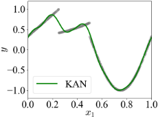
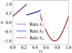
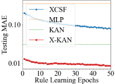
Since KAN is based on KART, which is designed for continuous functions, it may struggle to approximate discontinuous functions effectively. To validate this hypothesis, we conducted experiments using 1,000 data points samples from a discontinuous function with jump discontinuity used in [Shoji et al., 2023], as shown in Fig. 3a. For details of the function, kindly refer to Appendix I. The experimental settings followed Section 4.1, except for P# = 0.0, r0 = 0.5, ϵ0 = 0.01, maximum training iterations of 50 epochs for XCSF and XKAN, and 50 epochs for MLP, KAN, and X-KAN's local KAN models. Figs. 3b and 3c show the prediction plots from the best trials of KAN and X-KAN, respectively. Fig. 3d illustrates the decrease of the testing MAE during rule learning for XCSF and X-KAN, with the final MAE values for MLP and KAN (dashed horizontal lines).
Fig. 3b demonstrates that KAN fails to detect discontinuities, instead producing a smooth continuous function approximation. In contrast, Fig. 3c shows that X-KAN successfully identifies discontinuities and performs piecewise function approximation using three rules. The decreasing MAE trends by XCSF and X-KAN in Fig. 3d validate the effectiveness of local approximation.
These results demonstrate X-KAN's ability to handle dis-
(a) Training dataset
(b) Prediction results of KAN (c) Prediction results of X-KAN
(d) Testing MAE trends
| TRAINING MAE | TESTING MAE | #RULES IN PC | ||||
|---|---|---|---|---|---|---|
| X-KAN | X-KANκ | X-KAN | X-KANκ | X-KAN | X-KANκ | |
| f1 | 0.10780 | 0.08943 + | 0.16970 | 0.16880 ∼ | 9.200 | 18.60 - |
| f2 | 0.07356 | 0.07860 ∼ | 0.12730 | 0.12940 ∼ | 10.50 | 16.30 - |
| f3 | 0.01927 | 0.01949 ∼ | 0.02379 | 0.02397 ∼ | 4.867 | 9.633 - |
| f4 | 0.05171 | 0.04586 ∼ | 0.06922 | 0.06070 ∼ | 6.400 | 11.83 - |
| ASN | 0.03548 | 0.03073 + | 0.05533 | 0.05461 ∼ | 7.900 | 19.97 - |
| CCPP | 0.05691 | 0.05971 ∼ | 0.07871 | 0.08174 - | 7.800 | 17.53 - |
| CS | 0.02687 | 0.02497 ∼ | 0.07842 | 0.08014 ∼ | 7.900 | 17.40 - |
| EEC | 0.01561 | 0.01490 ∼ | 0.02729 | 0.03004 - | 2.667 | 7.367 - |
| Rank | 1.62 | 1.38↑ | 1.38 | 1.62↓ | 1.00 | 2.00↓† |
| +/-/ ∼ | - | 2/0/6 | - | 0/2/6 | - | 0/8/0 |
| p-value | - | 0.383 | - | 0.547 | - | 0.00781 |
Table 2: Comparison of fitness functions: X-KAN (accuracy and generality) vs. X-KANκ (accuracy only). Notation follows Table 1.
continuous functions through its adaptive partitioning approach, overcoming a fundamental limitation of KAN.
5.2 Role of Generality in Fitness
In Table 1, X-KAN never shows higher testing MAE than KAN. This high performance can be attributed to X-KAN (XCSF)'s fundamental principle of assigning fitness based on both accuracy κk and generality numk . To validate this hypothesis, we conducted experiments comparing X-KAN against its variant that assigns fitness solely based on accuracy (denoted as X-KANκ). For X-KANκ, the fitness update rule was simplified to F k ← κk . The experimental settings followed Section 4.1.
In Table 2, X-KANκ achieved significantly lower training MAE than X-KAN on two problems (f1, ASN). However, for testing MAE, X-KANκ performed significantly worse than X-KAN on two problems (CCPP, EEC). This performance degradation can be attributed to the increased probability of selecting parent rules with high accuracy but low generality (overfitting to training data) when generality is not considered in fitness calculation. Consequently, X-KANκ generated approximately twice as many rules as X-KAN due to reduced generalization pressure.
These findings demonstrate that considering both accuracy and generality, as implemented in XCSF and X-KAN, is crucial for improving generalization performance in evolutionary rule-based machine learning models.
5.3 Runtime Analysis
Fig. 4 shows the average runtime per trial under an experimental environment running Ubuntu 24.04.1 LTS with an Intel® Core™ i9-13900F CPU (5.60 GHz) and 32GB RAM.
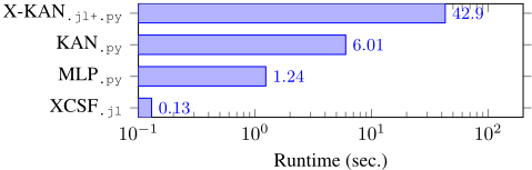
While MLP, KAN, and local KAN models in X-KAN were implemented in Python by the original KAN authors, the XCSF and X-KAN frameworks were implemented in Julia [Bezanson et al., 2017] by the authors. X-KAN calls Pythonbased local KAN models from its Julia framework. Note that, due to the mixed-use of programming languages, the runtime comparisons should be interpreted with caution.
As shown in Fig. 4, KAN requires approximately five times more runtime than MLP, mainly due to the computational overhead of recursive B-spline functions [Qiu et al., 2024]. Furthermore, X-KAN requires approximately seven times more runtime than KAN, as each rule's consequent implements a separate KAN model that must be trained.
One idea to decrease the runtime of X-KAN is to decrease the number of rules by increasing the generality of each rule. For example, dynamic adjustment of the target error threshold ϵ0 used in subsumption operations [Hansmeier et al., 2020] can reduce the total number of rules and shorten runtime.
6 Concluding Remarks
We introduced X-KAN which optimizes multiple local KAN models through an evolutionary framework based on XCSF. By defining local regions via rule antecedents and implementing local KAN models as rule consequents, X-KAN effectively combines KAN's expressiveness with XCSF's adaptive partitioning capability. Our experimental results showed that X-KAN significantly outperforms XCSF, MLP, and KAN for various function approximation problems with 7.2 rules on average. This improvement stems from X-KAN (XCSF)'s principle of assigning fitness based on both accuracy and generality, ensuring high generalization performance.
Future work will explore extending X-KAN as a piecewise symbolic regressor capable of extracting interpretable expressions inspired by [Chen et al., 2024; Liu et al., 2024].
Acknowledgments
This work was supported by JSPS KAKENHI (Grant Nos. JP23KJ0993, JP25K03195), National Natural Science Foundation of China (Grant No. 62376115), and Guangdong Provincial Key Laboratory (Grant No. 2020B121201001).
@inproceedings{ijcai2025p993,
  title     = {X-KAN: Optimizing Local Kolmogorov-Arnold Networks via Evolutionary Rule-Based Machine Learning},
  author    = {Shiraishi, Hiroki and Ishibuchi, Hisao and Nakata, Masaya},
  booktitle = {Proceedings of the Thirty-Fourth International Joint Conference on
               Artificial Intelligence, {IJCAI-25}},
  publisher = {International Joint Conferences on Artificial Intelligence Organization},
  editor    = {James Kwok},
  pages     = {8930--8938},
  year      = {2025},
  month     = {8},
  note      = {Main Track},
  doi       = {10.24963/ijcai.2025/993},
  url       = {https://doi.org/10.24963/ijcai.2025/993},
}
TY - CPAPER TI - X-KAN: Optimizing Local Kolmogorov-Arnold Networks via Evolutionary Rule-Based Machine Learning AU - Shiraishi, Hiroki AU - Ishibuchi, Hisao AU - Nakata, Masaya T2 - Proceedings of the Thirty-Fourth International Joint Conference on Artificial Intelligence, IJCAI-25 PB - International Joint Conferences on Artificial Intelligence Organization PY - 2025 SP - 8930 EP - 8938 DO - 10.24963/ijcai.2025/993 UR - https://doi.org/10.24963/ijcai.2025/993 ER -Copied
Machine-readable versions of this paper, for tools and AI agents:





