Sufficient Decision Proxies for Decision-Focused Learning

1 Introduction

Both in our daily life and in large-scale problems, we often make decisions under uncertainty. Imagine packing your suitcase or finding the best travel route when going to a conference. To make the right decision, we use available data that correlate with what is uncertain: e.g. we use seasonal weather patterns to predict the weather and decide if an umbrella is needed. We are trying to solve a contextual optimization or 'predict-then-optimize' problem: making predictions based on contextual information, which we then use for optimization (i.e., decision making). Since our goal is to make the best decision, we do not care about the predictions by themselves, but only about the decision they lead to. This is the main premise of decision-focused learning (DFL): learning a predictive model that optimizes for decision quality instead of prediction accuracy.

Defining our setting more formally: Observing contextual information in the form of feature values z ∈ Z, the goal of the decision maker is to find optimal decision x from constrained set X by solving the following problem:

where Cz is an unknown probability distribution. Since both c and Cz are unknown, learning a predictive model ϕθ(·) for c is a natural approach to the problem, assuming we have data with z, c pairs. After training, once new contextual information z is observed, we can predict an estimated scenario ˆ c = ϕθ(z). We do this because we would like to predict the realized value of c, i.e., the specific value that c will take in this empirical observation of z. If we do this successfully, we will get the empirical optimal decision by solving the deterministic approximation (proxy) of the true optimization problem in Equation (1): argminx∈X f(ˆ c, x). However, since the true c is stochastic and its distribution Cz is unknown, the empirical optimal decision is not necessarily the same as the true optimal decision based on Equation (1).

In certain settings it has been proven that a single estimated scenario and deterministic proxy allow for optimal decisionmaking, such as when uncertainty is linear in the objective [Elmachtoub and Grigas, 2022], or for certain fixed recourse, fixed costs two-stage stochastic problems [Homem-de Mello et al., 2026]. However, it has not been studied when a deterministic proxy leads to suboptimal decision-making, and how we can effectively apply DFL in this case. We address this gap in literature by contributing the following:

1. We provide sufficient and necessary conditions for when deterministic decision proxies are suboptimal and present problem classes where these conditions are met.
2. We present alternative decision proxies that adhere to sufficient conditions allowing for optimal decisionmaking, with little or no compromise on complexity.
3. We analyze continuous and discrete problems where deterministic proxies are suboptimal and show the effectiveness of the proposed proxies.

2 ProblemFormulation

The aim in a contextual optimization setting is to go from context z to optimal decision x∗ (z), by finding a mapping or policy π : Z → X. Due to the structure of the (potentially combinatorial) optimization problem x∗ (·), it is challenging to learn this complete end-to-end mapping directly [Bengio et al., 2021]. Considering it as separate prediction and optimization problems (predict-then-optimize) is practical, as both problems have been studied extensively [Sadana et al., 2025]. From the prediction problem perspective, assuming data with feature-label pairs z, c available, a typical learning would be to train predictor ϕθ : Z → C in a supervised manner by minimizing its predictive error (e.g., mean squared error: ||c-ˆ c||22 ). We will refer to this approach as predictionfocused learning (PFL). By contrast, DFL aims at learning a predictive model that minimizes decision error, taking the downstream optimization problem into account. Decision error is a measure of the difference between empirical optimal decision xD(c) and the obtained decision based on the prediction xD(ˆ c) (e.g., regret: f(c, xD(ˆ c)) - f(c, xD(c))). Here xD : C → X is the (single scenario) deterministic proxy of stochastic optimization problem x∗ (·) from (1):

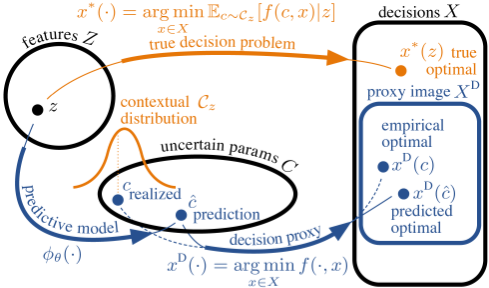
Both learning methods lead to a policy πD = xD ◦ ϕθ. It is natural to consider this deterministic proxy, since in practice we only have data available and therefore do not have Cz to compute x∗ (z) directly. We observe realized pairs z, c, that have an accompanied empirical optimal xD(c). However, at inference time, x∗ (z) is the optimal decision and there is no guarantee that xD(·) is able to equal x∗ (z). Proxy xD(·) can be limited to a subset of the feasible space XD ⊂ X due to its structure, which means that x∗ (z) is unattainable if it lies outside XD . Figure 1 shows a schematic representation of this potential problem. We give an illustrative example.

Example 1. Suboptimal investing based on the stockexchange paradox by Kibzun and Kan [1996]. Assume we have some capital that we want to grow in the coming t years. Every year, we can deposit capital in a bank with fixed rate of return β = 0.05 and we can purchase shares with an uncertain rate of return c ∼ U[-1, 1.7] (continuous uniformly distributed). If our aim is to maximize the next period's return, we will invest our whole capital in shares, since E[c] = 0.35 > 0.05. However, this leads to a negative expected growth rate:

Because of this, investing all capital in shares every period will make the probability of ruin, i.e., losing all capital at some point, converge to 1.

This is considered the stock-exchange paradox, where the Kelly strategy [Kelly, 1956] is being considered as solving:

Given c ∼ U[-1, 1.7] and β = 0.05, we get x∗ ≈ 0.465.

Now, if we look at the deterministic proxy of the problem, it will become clear that we cannot find the optimal decision:

Since ln(·) is a monotonically increasing function, we get: xD(ˆ c) = 1 when ˆ c < β & xD(ˆ c) = 0 when ˆ c > β. Hence true optimal decision x∗≈ 0.465 cannot be obtained.

2.1 Contextual Value of the Stochastic Solution

To more clearly present theory on the suboptimality of deterministic proxies, we extend the concept of value of the stochastic solution [Birge, 1982] to a contextual optimization setting. This concept is introduced as a measure for the value of solving a stochastic optimization problem as compared to solving a deterministic proxy with the uncertain variables replaced by their expectation. This is useful because in practice it is both harder to estimate the uncertain variables distribution (compared to its expectation) and more complex to solve a stochastic optimization problem. Here it gives us some clear structure to prove strict differences between solving a deterministic or stochastic contextual optimization problem. We first define the value of the true optimal decision based on Equation (1):

When we apply PFL, the predictive error is minimized if we are able to exactly estimate ¯ cz = Ec∼Cz [c|z]. Assuming that we can find this estimate, the value of a PFL decision is:

In the case of DFL the decision error is minimized. Assuming that we can find ˆ cz that minimizes the decision error, the value of the DFL decision is:

We have V∗ ≤ VDFL ≤ VPFL. The first inequality holds because in V∗ we directly minimize over the input of f(c, ·), x ∈ X, compared to minimizing over the argument of a function with codomain X, resulting in the same input of f(c, ·). The second inequality holds because we take minimizer ˆ cz ∈ C instead of ¯ cz ∈ C. Both inequalities hold for any z. This means that if there exists a z with non-zero probability mass for which one of the inequalities is strict, this inequality remains strict in expectation.

The value of using DFL over PFL VPFL - VDFL is highly relevant for predict-then-optimize problems. A general consensus is that this value increases with predictive error [Mandi et al., 2024], as the higher the predictive error the more important it is to learn such that decision quality is least affected. Additionally, Cameron et al. [2022] show that VPFL -VDFL is also influenced by dependencies between multiple uncertain variables: Predicting marginal expectations using PFL can cause theoretically unbounded worse performance compared to DFL.

In this work we are interested in the difference between the value of using DFL with a deterministic proxy VDFL and true optimal value V∗ : VDFL - V∗ . Due to DFL's end-to-end learning approach, proxy xD(·) has not been considered as limiting in its performance, even in more complex stochastic settings [Silvestri et al., 2026; van den Houten et al., 2024]. In the following we will identify cases when VDFL -V∗ > 0.

3 Suboptimal Deterministic Decision Proxies

This section presents cases where DFL with a deterministic proxy is provably suboptimal (VDFL > V∗ ). We first present theorems for the cases where V∗ = VDFL = VPFL and V∗ = VDFL < VPFL. Proofs are presented in the Appendix.

Theorem 1. There exists at least one optimal singlescenario w.r.t. Equation (1) if ∀z ∈ Z, Ec∼Cz [f(c, x)|z] = f(Ec∼Cz [c|z], x), i.e., Jensen's inequality renders an equality. In this case, an optimal single-scenario is ¯ cz = Ec∼Cz [c|z]. We have V∗ = VDFL = VPFL.

The most common application of Theorem 1 is when f(c, x) is linear in c, ∀x ∈ X. If Jensen's inequality is strict, and hence both functions have different minimizers, PFL becomes provably suboptimal:

Now we related this to VDFL, by presenting a sufficient condition for when a decision proxy allows for optimal decisionmaking, i.e., an optimal single-scenario exists.

Theorem 3. Deterministic proxy xD allows for optimal decision-making if xD(·) : C → X is surjective, i.e., ∀x ∈ X, ∃ˆ c ∈ C : xD(ˆ c) = x. We have V∗ = VDFL.

In other words: When xD is surjective, it is expressive enough to attain any feasible decision x ∈ X, which includes optimal x∗ (z). Theorem 2 and Theorem 3 demonstrate a theoretical case where PFL is inferior to DFL. The result that V∗ = VDFL, based on xD(·) being surjective, shows the flexibility of DFL: it allows for learning predictions that work well w.r.t. the true optimization problem. On the other hand, if the deterministic proxy is not able to reach stochastically optimal decisions, using this proxy is guaranteed to be suboptimal. This is the main intuition behind suboptimality of the deterministic proxy, and occurs when we have decision dominance:

Definition 1. Decision x ∈ X is (scenario-wise) dominated if ∀c ∈ C, ∃ (different) ˆx ∈ X s.t. f(c, ˆx) < f(c, x).

1 Notation is slightly abused here, as the minima's arguments are not necessarily unique. Technically these must be disjoint sets.

Note that this definition is based on the objective function f(·), which means that this property does not relate decisions w.r.t. the true stochastic problem in Equation (1).

Lemma 1. If there exists a scenario-wise dominated x ∈ X, proxy xD(c) = argminx∈X f(c, x) is not surjective.

Lemma 1 holds because dominated decisions can not be reached, violating the property of surjectivity. However, nonsurjectivity is not a sufficient condition for a proxy to be suboptimal. What is a sufficient and necessary condition is true optimal decision x∗ (z) being scenario-wise dominated, as the next theorem expresses.

Theorem 4. Proxy xD(·) is suboptimal if and only if there exists a feature value z ∈ Z for which true optimal x∗ (z) is scenario-wise dominated. We have V∗ < VDFL.

Despite not having access to x∗ (z), based on objective function f's characteristics we can prove that dominance occurs for certain continuous decision problems, i.e., when the feasibility set is compact (closed and bounded) and objective function f is continuous. After this we present a class of discrete problems where it is more natural to occur.

3.1 Continuous Optimization

The main result for continuous optimization problems is the following: Depending on the shape of objective function f(c, x) and expected objective function g(x) := Ec∼Cz [f(c, x)|z], it can occur that ∀c ∈ C the minimizer of f(c, x) lies on the boundary of X, while the minimizer of g(x) lies in the interior of X. In this case, all interior decisions are dominated by boundary decisions. In Example 1, we observe that the true objective function is convex non-monotonic in x, while the deterministic proxy objective function is strictly monotonic in x. Because of this the optimal decision according to the proxy lies on the boundary of the feasibility space, while the true optimal decision lies in the interior. This results in both decisions never coinciding. Example 1 has single-variable functions, but since we are working with multivariate functions in general, we first give a monotonicity definition for multivariate functions.

Definition 2. Let f : X → R,X ⊂ Rm be a multivariate function. f is (strictly) coordinate-wise (non)monotonic if ∀i ∈ {1, . . . ,m} we have that for any fixed variables {¯x1, . . . , ¯xi-1, ¯xi+1, . . . ¯xm} ∈ Rm-1 , f(¯x1, . . . , xi, . . . , ¯xm) is (strictly) (non-)monotonic in xi.

Coordinate-wise monotonicity allows the function to be decreasing in some variables while increasing in others.

Theorem 5. Given two continuous (objective) functions f : C,X → R, g : X → R, with g(x) := Ec∼Cz [f(c, x)|z], and (feasibility set) X is compact, i.e., closed and bounded, and has a nonempty interior. If f(c, x) is strictly coordinatewise monotonic in x for all c ∈ C, and g(x) is convex and coordinate-wise non-monotonic, then V∗ < VDFL.

In practice the constraints that define X can cause a lower intrinsic dimension and therefore an empty interior. However, in the Appendix we prove that the same result holds.

Example 2. Continuous objective functions with(out) suboptimal deterministic proxy. (Assuming X is compact.)

Objective f(c, x) = cT x does not satisfy the conditions of Theorem 5, since g(x) = Ec∼Cz [cT x|z] = Ec∼Cz [c|z]T x is linear in x for any distribution Cz and therefore not coordinate-wise non-monotonic. Similarly 1 cT x and (cT x)n with even n's do not satisfy the conditions of Theorem 5 as they are also not coordinate-wise non-monotonic.

Objective f (c, x) = - log(cT x) does satisfy the conditions of Theorem 5 for at least some distributions Cz. This is because

-log(cT x) is strictly coordinate-wise monotonic ∀c ∈ C, because for any ci > 0, increasing xi increases log(cT x), and for any ci < 0, decreasing xi decreases log(cT x). On the other hand, g(x) can be strictly convex with a minimum in the interior, depending on the distribution Cz (see Example 1). Similarly √cT x, ecT x and (cx)n with odd n's satisfy the conditions of Theorem 5.

So far we have derived properties for the structure of the optimization problem to show suboptimality. Based on the function examples, one could argue that the types of functions for which this occurs are not common. However, there is an important class of practical optimization problem that typically have complex, non-smooth objective functions.

3.2 Two-Stage Stochastic Optimization Problems

A practical class of optimization problems where a deterministic proxy can be suboptimal is the class of two-stage stochastic optimization problems. This two-stage formulation is of particular interest in optimization literature [Birge and Louveaux, 2011], as it is effective in modeling real-world problems under uncertainty. These problems consist of making first-stage decisions x that are taken before uncertain parameters c are realized and second-stage decisions y that denote some recourse action after uncertain parameters c are realized. The general formulation is:

The relevance of this formulation comes from the fact that in practice the realization of uncertainty leads to some action: if we did not bring an umbrella, we can buy a new one. These recourse actions include additional costs compared to what was initially decided. One can model the problem in a way it has relatively complete recourse, i.e., the second stage is feasible for any feasible first-stage decision. This is one of the main benefits of two-stage stochastic optimization, as other uncertain problem formulations like (distributionally) robust optimization or chance constraints [Charnes and Cooper, 1962] can only ensure feasibility for a specific set of uncertain value realizations or with a certain probability. Specifically, models with a linear second stage are commonly used: Equation (2) with g(c, x, y) = q(c)T y and Y (c, x) = {y : T (c)x + U(c)y = h(c)}.

Homem-de Mello et al. [2026] showed that for these problems with fixed costs and fixed recourse, i.e., q(c) = q and U(c) = U being independent of c, an optimal single-scenario exists. The proof is based on the assumption that each entry of vector h(c) is dependent on c, but when it has independent fixed entries, an optimal single-scenario does not necessarily exist. We demonstrate this with an example based on the weighted-set multi-cover problem in the Appendix. This shows that even for this class of problems it is relevant to consider the used decision proxy.

4 Sufficient Decision Proxies

In the previous section we saw that a sufficient condition for a proxy to be able to lead to an optimal decision is that it is expressive enough. In this section we present proxies that can adhere to this condition, when a deterministic proxy does not. We also discuss why an intuitive choice, using a parameterized distribution proxy, is most often not effective. Recall that in a contextual optimization problem, the input to the chosen proxy x(·) is the output of the predictive model ϕθ(·), so each proxy asks for a different output from the predictive model. Applying DFL we train this predictive model to get a decision-quality maximizing policy π : Z → X, π = x ◦ ϕθ w.r.t. Equation (1), instead of aiming for the most accurate estimation of uncertain parameters c or distribution Cz.

4.1 Scenario-Based Proxy

Based on Theorem 4 we know that in certain cases proxy xD(·) is suboptimal. Since this deterministic variant is introduced to approximate decision problem of interest in Equation (1), we consider an alternative approximation based on the principle of sample average approximation (SAA) [Kleywegt et al., 2002]:

Note that xD(·) = xS1 (·). SAA is used to approximately solve stochastic optimization problems, when the uncertain parameter distribution is known but does not lead to a solvable optimization problem (non closed-form objective). This approach works by sampling and subsequently solving the SAA. The SAA converges to the true stochastic optimization problem as the number of samples goes to infinity. In the contextual optimization setting this results in the following theorem:

Theorem6 (Kimet al. [2015]). SupposeA ⊂X is nonempty and compact, such that (i) x∗ (z) ∈ A, (ii) for sufficiently large n, xSn ∈ A and (iii) suppose that f(c, ·) is continuous at x a.s. for any x ∈ X, and that there exists δ > 0 such that the family of random variables {f(c, y) : ||y - x|| < δ} is uniformly integrable. Then xSn (·) → x∗ (z).

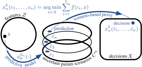
Based on this theorem, as long as we pick n large enough we can learn to closely approximate the true distribution and get the optimal decision. In a DFL pipeline however, it would be too costly to pick a high value of n. Fortunately, the main benefit of DFL is that it can learn to produce high-quality decisions as long as the decision proxy is expressive enough. To achieve this, we predict the scenarios directly instead of sampling them as done in SAA. This results in the following predictor ϕSn θ : Z → C n , and scenario-based policy πSn = xSn ◦ ϕSn θ . In the experimental results we see that with as few as n = 2 scenarios the scenario-based proxy leads to significantly better decisions than the deterministic proxy. This shows that DFL eliminates the need of using many samples. Figure 2 shows a schematic representation of the scenario-based proxy.

4.2 Quadratic Proxy

Instead of trying to approximate Equation (1) better, we can also look at the problem from the other perspective: Based on the earlier-developed theory we can design a proxy that has sufficient conditions that allow for optimal decision-making. We can do this by replacing the objective function f(·). First, we generalize the first part of Theorem 3:

Theorem 7. Consider a function x(·) : Ξ →X. An optimal prediction w.r.t. Equation (1) exists if x(·) is surjective, i.e., ∀x ∈ X, ∃ˆ ξ ∈ Ξ : x(ˆ ξ) = x.

Proof. Take an arbitrary z, with optimal decision x∗ (z). Given that x(·) is surjective, ∃ˆ ξ ∈ Ξ s.t. x(ˆ ξ) = x∗ (z).

We now introduce a surjective function for this setting, which coincides with the quadratic approximation proposed by Veviurko et al. [2024] to deal with the zero-gradient problem and is the projection predictions on the decision space.

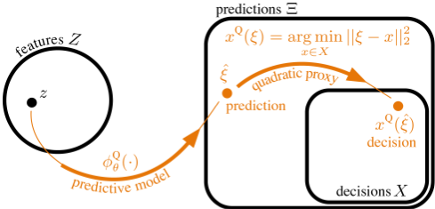
This proxy is surjective by design, as for arbitrary x ∈ X, taking ˆ ξ = x leads to xQ(ˆ ξ) = x. This leads us to using predictive model ϕQθ : Z → Ξ, where Ξ = Rdim(X) , and quadratic policy πQ = xQ ◦ ϕQθ . Figure 3 shows a schematic representation of the quadratic proxy.

We elaborate more on the rationale of this proxy xQ(·): it has a strictly convex objective function, while adhering to the constraints of the problem (feasibility set X). This means we can train with DFL and always reach feasible decisions. Based on the assumption of the predictive model being a universal approximator, the objective function does not have to mimic the true objective function in Equation (1). This is because an optimal decision always lies in some minimum, and this minimum can be approximated by a quadratic function. The DFL pipeline should ensure the predictor learns to predict in the right area. In this case, this area is in the same space as the decisions, where the proxy projects the prediction in the feasibility space. So effectively we are predicting directly from features to approximate decisions, without considering the uncertain parameters in between. Most approaches in this category have some correction step to make the decision feasible [Kotary et al., 2024]. In this case this can be considered to be the decision proxy itself.

4.3 Parameterized Distribution Proxy

Since we argue that deterministic proxies and therefore single-scenario predictions can be suboptimal, an intuitive approach would be to predict a distribution and use this to approximate Cz in Equation (1). This leads to the following decision proxy, with β ∈ B the parameters of the chosen distribution P and pβ(·) its density function:

This leads to using predictive model ϕPθ : Z → B and policy πP = xP ◦ ϕPθ . This approach is discussed as it is effective when the decision proxy has a closed-form, as in one of the experiments by Donti et al. [2017] where the underlying distribution is Gaussian. In practice however, the chosen distribution is unlikely to result in a closed-form integral, especially when problems are more complex, such as the class of problems we aim to tackle. It is still possible to approximate this proxy by discretizing the integral and using SAA. However, this indirect approach of first predicting a distribution and then extracting scenarios is a more restricted version of the scenario-based approach, always resulting in poorer performance. Therefore, we did not include the results.

4.4 Complexity

All presented policies have a different combination of predictors and decision proxies. Table 1 summarizes the policies by denoting the prediction space and the number of decision variables in a two-stage stochastic optimization setting. This number correlates highly with the number of problem constraints, as any constraint involving a second-stage decision is considered for each scenario. In general more decision variables and constraints increase the complexity of the decision proxy. Despite the focus here being on achieving high-quality policies, the complexity of the proxy is highly relevant as it is solved for each data point and epoch in a DFL pipeline.

The prediction space has less impact. The size of this space impacts the number of parameters of the predictive model. Since in general we (can) use neural networks with vastly more parameters than the dimension of the prediction space, this does not change much. What is more of an open question is whether the prediction space influences the complexity of learning a high-quality policy. In some problems dim(X) is significantly different from dim(C), which leads to the question if πQ is harder to learn than πSn . We see small differences in the experiments that are in line with this hypothesis.

5 Experimental Evaluation

To experimentally evaluate the proposed approaches as alternatives to a deterministic proxy, we consider one continuous and two discrete problems. We use three baselines: deterministic proxy learned using DFL πD , deterministic proxy learned using PFL πD PFL and a PFL learned model using SAA at inference πS PFL . In the PFL approaches we train on mean squared error, where πSn PFL uses the same learned predictive model as PFL ϕθ, but evaluates based on an SAA approximation xSn . This is done by using a residual-based distribution [Sadana et al., 2025], using empirical additive errors [Deng and Sen, 2022]: taking the predictions as mean, and adding samples from the observed residuals from the validation set. We use n = 16, so πS16 PFL in all problems. We compare the baselines with our proposed approaches: πQ , πSn , with n ∈ {2, 8, 16}. For the continuous problem we apply DFL using differentiable convex layers [Agrawal et al., 2019] as the problem is differentiable. For the other problems we use score function gradient estimation [Silvestri et al., 2026], which is approximates gradients by using stochastic sampling and is therefore applicable to any non-differentiable problem. Regarding the predictors we use neural networks with 2 hidden layers of size 256 and LeakyReLU activation functions, a learning rate of 5 × 10-4 and batch size of 32. Each approach has the same number of epochs, which we consider enough to converge. The best performing model on validation is used for test. Adam optimizer is used for gradient descent and Gurobi [Gurobi Optimization, 2025] as the solver. Code is available 2 , based on PyDFLT [Schutte et al., 2026]. For further experimental details please refer to the Appendix.

We consider problems where the deterministic proxy is not sufficient. Since literature so far has omitted these problems, we modified problems from literature to fit this requirement.

Portfolio optimization. As considered in earlier work on DFL [Wang et al., 2020; Veviurko et al., 2024], we consider a portfolio problem based on data from Quandl [2023]. Instead of balancing return and risk, we maximize the long-term expected value of the portfolio using the Kelly strategy [Kelly, 1956]. This makes the problem a multivariate version of Example 1. We determine the fixed rate of return β to be the median of all the fourth highest returns per training instance. Since data is limited (2898 data points) we do not use different data splits, instead we randomly pick 10 different securities for each seed, running 10 different seeds. We use a train, validation, test split of 70%, 15%, 15%.

2 https://github.com/PyDFLT/PyDFLT/tree/ sufficient-decision-proxies-ijcai2026

Weighted-set multi-cover. We test on the WSMC problem as presented by Silvestri et al. [2026] with one adjustment: We allow removing single-item sets in the case of excess coverage for a partial return of costs, which makes the recourse similar to the common two-stage knapsack problem with uncertain weights [Kosuch and Lisser, 2011]. The deterministic proxy can be suboptimal in this case (see Appendix for example). We run 10 random seeds and for train, validation and test set sizes, we use 1000, 250 and 1250.

Probabilistic traveling salesperson. Finally we test on a two-stage probabilistic traveling salesperson (PTSP). Probabilistic vehicle routing problems have been studied since Tillman [1969], with PTSP specifically introduced by [Jaillet, 1985], and are still highly relevant [Oyola et al., 2018]. The goal of the PTSP is to plan a route along a known set of customers while minimizing transportation costs, but it is uncertain which customers require service. Missing a customer who requires service incurs a penalty (based on going backand-forth to the depot, which is a typical recourse choice [Oyola et al., 2018]). In this two-stage version, one is allowed to add direct trips to customers, similar to allowing crowdsourcing Santini et al. [2022]. After it becomes known which customers require service, these direct trips can be canceled in the second stage if they are not required. This makes the problem such that in a given scenario, direct trips are always dominated, but given uncertainty they have the benefit of incurring low costs if canceled. We run 10 seeds and for train, validation and test set sizes, we use 1000, 250 and 1250.

5.1 Results

Figure 4 shows the final results, while Figure 5 visualizes the learning. We use a paired t-test (5% significance level) to compare our proposed methods with the deterministic proxy baseline, and they performed significantly better in all cases.

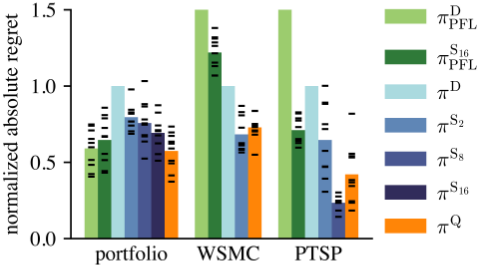
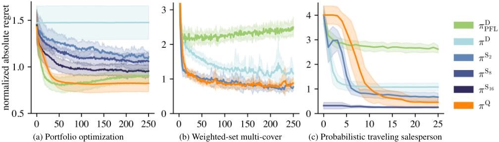
We see that πQ performs best or second best in all cases. In both WSMC and PTSP the dimension of decision variables is greater than the dimension of uncertain variables. Since this makes πQ learn the same relationship through a mapping with higher dimension, it could be the reason the scenariobased approach performs slightly better. In general we see that more scenarios for the scenario-based approach results in better performance. For portfolio, Figure 5a shows that πD is not able to learn at all. This is primarily caused by having zero-gradients. A higher number of scenarios here results in more effective gradients. The most notable part about the WSMC is that the learning curves have high variance. This is inherent to the score function gradient estimation approach. For PTSP this is not as pronounced, due to the small problem size and therefore less complex decision landscape. However, for PTSP we do observe higher variance in the test results for πQ and πS 2 , suggesting problem-dependent lower robustness.

6 Discussion and RelatedWork

We formally showed cases when deterministic proxies are suboptimal, even in a DFL setting, and introduce effective alternative proxies. This is another step in understanding the applicability of DFL, after Cameron et al. [2022] consider when PFL is worse compared to DFL and Homem-de Mello et al. [2026] show for a certain class of problems that an optimal single-scenario exists. Similarly, Schutte et al. [2024] discuss the importance of the decision proxy by highlighting the difference between the empirical (deterministic) problem and the true stochastic problem, and introduce loss functions that generalize better. Furthermore, [Wilder et al., 2019] introduced a continuous relaxation proxy to speed up DFL, using a quadratic regularization term on the decision vector.

There are several works that consider the true problem as stochastic and use distribution-based decision proxies. These works differ from our work in that we provide theoretical backing on when a deterministic proxy is suboptimal, as well as propose alternatives based on this theory that keep complexity low. Donti et al. [2017] tackle a problem that has a differentiable formulation when assuming the uncertainty is Gaussian. Alternatively they assume the uncertain parameter has finite discrete support, having the predictive model output probabilities for these discrete scenarios. This is a similar assumption as done by Qi et al. [2025], which is quite limiting as uncertain parameters are often continuous and multi-dimensional, requiring to decide on some discretization that is representative without having too many scenarios. Our scenario-based approach learns representative scenarios and only requires to decide the number of scenarios up front. Elmachtoub et al. [2025] also include a distributionbased approach, assuming a parameterized family of distributions. They show that when the distribution is misspecified, distributional DFL (contextual integrated-estimationoptimization) outperforms distributional PFL (estimate-thenoptimize), while in a well-specified distribution case the result is opposite. Jia et al. [2025] use scenarios in a predictthen-optimize routing problem, but do not train end-to-end.

Stochasticity is also used to obtain gradients when they do no exist or are zero, but in these cases the deterministic proxy is applied at inference [Berthet et al., 2020; Silvestri et al., 2026]. The same is done at inference by Hu et al. [2023], who consider uncertainty in the constraints and model infeasibility using penalties. We refer the reader to [Qi and Shen, 2022] for an operations management perspective on DFL, and [Mandi et al., 2024] for a general DFL survey.

7 Conclusions

A prevailing assumption in decision-focused learning is that there exists a single-scenario problem approximation that allows for optimal decision-making. While this is a valid assumption in a wide class of problems, this paper investigates for the first time general theoretical properties of problems for which this assumption is violated. Based on these properties we derive requirements for problem approximations that are sufficient to reach optimal decisions. On three problems we empirically showed the value of the proposed approaches. Future work includes studying problems where parameterized distributions can easily be assumed and problems from practice, to evaluate the applicability of DFL and different proxies. Given the strong performance of the quadratic proxy, it raises the question how relevant the true objective is in DFL.

Acknowledgments

We thank the reviewers for their suggestions. This work was partially supported by Epistemic AI and by TAILOR, both funded by EU Horizon 2020 under grants 964505 and 952215 respectively.