
From Diversity to Uniformity: Cross-modal Time Series Modeling with Dependent Channel Grouping
Proceedings of the Thirty-Fifth International Joint Conference on Artificial Intelligence. Main Track. Pages 2447-2455.
https://doi.org/10.24963/ijcai.2026/272
Keywords
- AI: Data Mining
- Data Mining: Mining spatial and/or temporal data
Abstract
Emerging foundation models have spurred growing interest in task-unspecific time series modeling, which can accommodate data from diverse domains and support various tasks. However, most existing methods still suffer from poor adaptability and generalization across cross-domain time series with varying feature dimensionalities. This study achieves unified time series modeling to transcend task and data boundaries, inspired by the recent advances in visual foundation models. We propose a universal cross-modal Time series modeling method named TimeIG, featuring Tailored Temporal Imaging and Dependent Channel Grouping. Specifically, TimeIG adopts the novel dependent channel grouping method to project heterogeneous time series into hierarchical spaces to identify representative features and learn inter-dependencies across variables. Then, a tailored temporal imaging method is proposed to generate carefully hand-crafted images from time series, facilitating complementary temporal-spatial feature extraction. Finally, a dual-branch module is designed to simultaneously model the sequential and visual data, enabling cross-modal alignment via the proposed Cross-Modal Attention and Dynamic Weighted-Averaging. Extensive experiments on real-world cross-domain time series datasets show that TimeIG consistently outperforms existing SOTA methods. The code of TimeIG is publicly available at https://github.com/missCmj/TimeIG.
- [Bagnall et al., 2018] Anthony Bagnall, Hoang Anh Dau, Ja- son Lines, Michael Flynn, James Large, Aaron Bostrom, Paul Southam, and Eamonn Keogh. The uea multivari- ate time series classification archive, 2018. arXiv preprint arXiv:1811.00075, 2018.
- [Bai et al., 2018] S. Bai, J. Z. Kolter, and V. Koltun. An empirical evaluation of generic convolutional and recur- rent networks for sequence modeling. arXiv preprint arXiv:1803.01271, 2018.
- [Campos et al., 2023] David Campos, Miao Zhang, Bin Yang, Tung Kieu, Chenjuan Guo, and Christian S Jensen. Lightts: Lightweight time series classification with adap- tive ensemble distillation. SIGMOD, 1(2):1-27, 2023.
- [Cao et al., 2024] Defu Cao, Furong Jia, Sercan Ö. Arik, Tomas Pfister, Yixiang Zheng, Wen Ye, and Yan Liu. Tempo: Prompt-based generative pre-trained transformer for time series forecasting. ICLR, 2024.
- [Challu et al., 2023] Cristian Challu, Kin G. Olivares, Boris N. Oreshkin, Federico Garza, Max Mergenthaler- Canseco, and Artur Dubrawski. Nhits: Neural hierarchical interpolation for time series forecasting. AAAI, 2023.
- [Chen and Zhao, 2024] Jiawei Chen and Chunhui Zhao. Ad- dressing spatial-temporal heterogeneity: General mixed time series analysis via latent continuity recovery and alignment. NeurIPS, 2024.
- [Chen et al., 2023] Yuhang Chen, Chaoyun Zhang, Minghua Ma, Yudong Liu, Ruomeng Ding, Bowen Li, Shilin He, Saravan Rajmohan, Qingwei Lin, and Dongmei Zhang. Imdiffusion: Imputed diffusion models for multivariate time series anomaly detection. PVLDB, 17(3):359-372, 2023.
- [Chen et al., 2025] Mouxiang Chen, Lefe Shen, Zhuo Li, Xi- aoyun Joy Wang, Jianling Sun, and Chenghao Liu. Vi- sionts: Visual masked autoencoders are free-lunch zero- shot time series forecasters. ICML, 2025.
- [Cheng et al., 2024] Yunyao Cheng, Peng Chen, Chenjuan Guo, Kai Zhao, Qingsong Wen, Bin Yang, and Christian S Jensen. Weakly guided adaptation for robust time series forecasting. PVLDB, 17(4):766-779, 2024.
- [Dempster et al., 2020] A. Dempster, F. Petitjean, and G. I. Webb. Rocket: exceptionally fast and accurate time series classification using random convolutional kernels. Data Mining and Knowledge Discovery, 34(5):1454- 1495, 2020.
- [Ekambaram et al., 2023] Vijay Ekambaram, Arindam Jati, Nam Nguyen, Phanwadee Sinthong, and Jayant Kalagnanam. Tsmixer: Lightweight mlp-mixer model for multivariate time series forecasting. In SIGKDD, pages 459-469, 2023.
- [Gao et al., 2024] Shanghua Gao, Teddy Koker, Owen Queen, Tom Hartvigsen, Theodoros Tsiligkaridis, and Marinka Zitnik. Units: A unified multi-task time series model. NeurIPS, 37:140589-140631, 2024.
- [Ghorbani et al., 2024] Ramin Ghorbani, Marcel JT Rein- ders, and David MJ Tax. Pate: Proximity-aware time series anomaly evaluation. In SIGKDD, pages 872-883, 2024.
- [Haoqing Wang, 2023] Zhihong Deng Haoqing Wang, Shibo Jie. Focus your attention when few-shot classifica- tion. NeurIPS, 2023.
- [Ismail Fawaz et al., 2020] H. Ismail Fawaz, B. Lucas, G. Forestier, C. Pelletier, D. F. Schmidt, and G. I. Webb. Inceptiontime: Finding alexnet for time series classifica- tion. Data Mining and Knowledge Discovery, 34(6):1936- 1962, 2020.
- [Jin et al., 2024] Ming Jin, Shiyu Wang, Lintao Ma, Zhix- uan Chu, James Y Zhang, Xiaoming Shi, Pin-Yu Chen, Yuxuan Liang, Yuan-Fang Li, Shirui Pan, et al. Time-llm: Time series forecasting by reprogramming large language models. ICLR, 2024.
- [Lai et al., 2018] G Lai, WC Chang, Y Yang, and H Liu. Modeling long-and short-term temporal patterns with deep neural networks. SIGIR, 2018.
- [Liang and Wang, 2024] Zhiyu Liang and Hongzhi Wang. Fedst: secure federated shapelet transformation for time series classification. VLDB, 33(5):1617-1641, 2024.
- [Liu et al., 2021] Chi Harold Liu, Chengzhe Piao, Xiaoxin Ma, Ye Yuan, Jian Tang, Guoren Wang, and Kin K Leung. Modeling citywide crowd flows using attentive convolu- tional lstm. In ICDE, pages 217-228, 2021.
- [Liu et al., 2024a] Q. Liu, P. Boniol, T. Palpanas, and J. Pa- parrizos. Time-series anomaly detection: Overview and new trends. VLDB, 17(12):4229-4232, 2024.
- [Liu et al., 2024b] Qinghua Liu, Paul Boniol, Themis Pal- panas, and John Paparrizos. Time-series anomaly detec- tion: Overview and new trends. PVLDB, 17(12):4229- 4232, 2024.
- [Liu et al., 2024c] Xu Liu, Junfeng Hu, Yuan Li, Shizhe Diao, Yuxuan Liang, Bryan Hooi, and Roger Zimmer- mann. Unitime: A language-empowered unified model for cross-domain time series forecasting. In WWW, pages 4095-4106, 2024.
- [Liu et al., 2024d] Yong Liu, Tengge Hu, Haoran Zhang, Haixu Wu, Shiyu Wang, Lintao Ma, and Mingsheng Long. itransformer: Inverted transformers are effective for time series forecasting. In ICLR, 2024.
- [Liu et al., 2024e] Yong Liu, Tengge Hu, Haoran Zhang, Haixu Wu, Shiyu Wang, Lintao Ma, and Mingsheng Long. itransformer: Inverted transformers are effective for time series forecasting. In ICLR, 2024.
- [Liu et al., 2024f] Yong Liu, Guo Qin, Xiangdong Huang, Jianmin Wang, and Mingsheng Long. Autotimes: Autore- gressive time series forecasters via large language models. NeurIPS, 2024.
- [Liu et al., 2024g] Yong Liu, Haoran Zhang, Chenyu Li, Xi- angdong Huang, Jianmin Wang, and Mingsheng Long. Timer: Generative pre-trained transformers are large time series models. ICLR, 2024.
- [Liu et al., 2025a] Chenxi Liu, Hao Miao, Qianxiong Xu, Shaowen Zhou, Cheng Long, Yan Zhao, Ziyue Li, and Rui Zhao. Efficient multivariate time series forecasting via calibrated language models with privileged knowledge distillation. In ICDE, pages 3165-3178, 2025.
- [Liu et al., 2025b] Chenxi Liu, Shaowen Zhou, Qianxiong Xu, Hao Miao, Cheng Long, Ziyue Li, and Rui Zhao. To- wards cross-modality modeling for time series analytics: A survey in the llm era. In IJCAI, 2025. IJCAI
- [Liu et al., 2025c] Yong Liu, Guo Qin, Xiangdong Huang, Jianmin Wang, and Mingsheng Long. Timer-xl: Long- context transformers for unified time series forecasting. ICLR, 2025.
- [Miao et al., 2024] Hao Miao, Yan Zhao, Chenjuan Guo, Bin Yang, Kai Zheng, Feiteng Huang, Jiandong Xie, and Christian S. Jensen. A unified replay-based continu- ous learning framework for spatio-temporal prediction on streaming data. In ICDE, 2024.
- [Nguyen et al., 2024] T. Nguyen, J. Jewik, H. Bansal, P. Sharma, and A. Grover. Climatelearn: Benchmark- ing machine learning for weather and climate modeling. NeurIPS, 36, 2024.
- [Ni et al., 2024] Jingchao Ni, Ziming Zhao, ChengAo Shen, Hanghang Tong, Dongjin Song, Wei Cheng, Dongsheng Luo, and Haifeng Chen. Harnessing vision models for time series analysis: A survey. In IJCAI, 2024. IJCAI
- [Nie et al., 2023] Yuqi Nie, Nam H. Nguyen, Phanwadee Sinthong, and Jayant Kalagnanam. A time series is worth 64 words: Long-term forecasting with transformers. ICLR, 2023.
- [Paul Boniol, 2020] Themis Palpanas Paul Boniol. Se- ries2graph: Graph-based subsequence anomaly detection for time series. VLDB, 2020.
- [Qiu et al., 2024] Xiangfei Qiu, Jilin Hu, Lekui Zhou, Xingjian Wu, Junyang Du, Buang Zhang, Chenjuan Guo, Aoying Zhou, Christian S Jensen, Zhenli Sheng, et al. Tfb: Towards comprehensive and fair benchmarking of time se- ries forecasting methods. VLDB, 17(9):2363-2377, 2024.
- [Shekhar and Williams, 2007] Shashank Shekhar and Billy M Williams. Adaptive seasonal time series models for forecasting short-term traffic flow. TRR, 2024(1):116- 125, 2007.
- [Shi et al., 2015] Xingjian Shi, Zhe Chen, Hao Wang, Dit- Yan Yeung, Wai-Kin Wong, and Wang-Chun Woo. Con- volutional LSTM network: A machine learning approach for precipitation nowcasting. NeuralIPS, 2015.
- [Shreshth Tuli, 2022] Nicholas R. Jennings Shreshth Tuli, Giuliano Casale. Tranad: Deep transformer networks for anomaly detection in multivariate time series data. VLDB, 2022.
- [Stellwagen and Tashman, 2013] Eric Stellwagen and Len Tashman. Arima: The models of box and jenkins. In Fore- sight: The International Journal of Applied Forecasting, volume 33, pages 28-33, 2013.
- [Tran et al., 2025] Viet-Hung Tran, Ngoc Phu Doan, Zichi Zhang, Tuan Pham, Phi Hung Nguyen, Xuan Hoang Nguyen, Hans Vandierendonck, Ira Assent, and Thai Son Mai. Mix: A multi-view time-frequency interactive ex- planation framework for time series classification. In NeurIPS, 2025.
- [Wu et al., 2021] Haixu Wu, Jiehui Xu, Jianmin Wang, and Mingsheng Long. Autoformer: Decomposition transform- ers with auto-correlation for long-term series forecasting. In NeurIPS, 2021.
- [Wu et al., 2023] Haixu Wu, Tengge Hu, Yong Liu, Hang Zhou, Jianmin Wang, and Mingsheng Long. Timesnet: Temporal 2d-variation modeling for general time series analysis. ICLR, 2023.
- [Xu et al., 2024] Ronghui Xu, Hao Miao, Senzhang Wang, Philip S. Yu, and Jianxin Wang. Pefad: A parameter- efficient federated framework for time series anomaly de- tection. In KDD, 2024.
- [Xu et al., 2025] Huibo Xu, Likang Wu, Xianquan Wang, Zhiding Liu, and Qi Liu. Tcdm: A temporal correlation- empowered diffusion model for time series forecasting. In IJCAI, 2025.
- [Yang et al., 2023] Yiyuan Yang, Chaoli Zhang, Qing- song Wen Tian Zhou, and Liang Sun. Dcdetector: Dual attention contrastive representation learning for time series anomaly detection. SIGKDD, 2023.
- [Yin et al., 2025] Jun Yin, Zhengxin Zeng, Mingzheng Li, Hao Yan, Chaozhuo Li, Weihao Han, Jianjin Zhang, Ruochen Liu, Hao Sun, Weiwei Deng, et al. Unleash llms potential for sequential recommendation by coordinating dual dynamic index mechanism. In WWW, 2025.
- [Zeng et al., 2021] A Zeng, M Chen, L Zhang, and Q Xu. Dlinear: Are transformers effective for time series fore- casting? AAAI, 2021.
- [Zhong et al., 2025] Siru Zhong, Weilin Ruan, Ming Jin, Huan Li, Qingsong Wen, and Yuxuan Liang. Time-vlm: Exploring multimodal vision-language models for aug- mented time series forecasting. ICML, 2025.
- [Zhou et al., 2021] Haoyi Zhou, Shanghang Zhang, Jieqi Peng, Shuai Zhang, Jianxin Li, Hui Xiong, and Wancai Zhang. Informer: Beyond efficient transformer for long sequence time-series forecasting. AAAI, 2021.
- [Zhou et al., 2022] Tian Zhou, Ziqing Ma, Qingsong Wen, Xue Wang, Liang Sun, and Rong Jin. Fedformer: Fre- quency enhanced decomposed transformer for long-term series forecasting. ICLR, 2022.
References were extracted automatically from the PDF and may contain errors.
Full text extracted automatically from the PDF; figures, tables and equations may differ. The PDF is the version of record.
1 Introduction
The proliferation of edge devices generates massive volumes of time series, enabling various time series analytical tasks [Liu et al., 2025b; Liu et al., 2024c], e.g., forecasting [Miao et al., 2024], classification [Tran et al., 2025], and anomaly detection [Xu et al., 2024]. We are seeing remarkable advances in deep learning that are successful at extracting information and creating value from time series [Liu et al., 2025b]. However, most existing methods assume the time series data are homogeneous with a consistent number of variables, which limits their adaptability to deal with the time series exhibiting high heterogeneity with varying feature dimensionalities. Such heterogeneity creates a critical bottleneck for a universal time-series modeling approach to generalize across analytical tasks.
∗Corresponding Author
Recent efforts in time series foundation models have attempted to address the heterogeneity issue [Gao et al., 2024; Cao et al., 2024; Chen and Zhao, 2024], which often treat each variable independently [Nie et al., 2023; Liu et al., 2024c], thereby ignoring the inter-variable dependencies [Gao et al., 2024]. More recently, image-based technologies have emerged to convert time series into visual representations, modeling temporal sequences as two-dimensional structures amenable to computer vision techniques [Wu et al., 2023; Zhong et al., 2025]. Especially, VisionTS [Chen et al., 2025] demonstrates that appropriately converting time series into visual representations can reveal essential time series features, e.g., trend, seasonality, and stationarity, thereby facilitating the capture of temporal dependencies. Nonetheless, image-based methods often fail to preserve the sequential nature and inter-variable relations key to understanding time series [Ni et al., 2024].
In this paper, we consider explicitly combining temporal sequence modeling with spatial image-based representations via multi-modal fusion. The explicit multi-modal integration is expected to digest more comprehensive temporalspatial information for more effective time series modeling. However, it is non-trivial to develop such a method due to the following challenges. First, it is challenging to model inter-variable dependencies among heterogeneous time series. It is expected to preserve intrinsic time series characteristics and enable effective knowledge transfer by aligning heterogeneous time series with varying dimensionalities across tasks. Second, it is difficult to achieve high-quality images with comprehensive information from the original time series. Third, it is important to carefully fuse complementary cross-modal temporal-spatial representations, as improper fusion can lead to excessive reliance on one modality and suboptimal performance. This study addresses the above challenges by developing a cross-modal modeling framework, entitled TimeIG, featuring dependent channel grouping and dual-branch temporal-spatial encoding.
TimeIG achieves a unified modality-aware framework for task-unspecific time series modeling that synergistically combines temporal sequence encoding with spatial-image-based representations through sophisticated cross-modal alignment. Specifically, to accommodate heterogeneous time series with varying numbers of variables, we propose a Dependent Channel Grouping module that identifies representative anchor channels to project diverse inputs into a standardized Kdimensional latent space regardless of original dimensionality. The Dependent Channel Grouping module aims to preserve the intrinsic dependencies among variables while providing a uniform representation for subsequent encoding.
Then, we carefully transform the unified time series into temporal images via tailored temporal imaging, which decomposes time series modeling into three complementary components: periodicity, relational matrix, and phaseamplitude. This decomposition reflects the fundamental mathematical properties of time series data-periodicity captures the cyclical patterns inherent in temporal phenomena, relational matrices encode the correlation structures among variables, and phase-amplitude analysis preserves the frequency domain characteristics crucial for understanding temporal dynamics. Next, we design Dual-branch Encoding, including time series encoding and temporal image encoding branches, to capture temporal dynamics and image-based spatial patterns simultaneously. The time series encoding branch captures sequential dynamics through patch-based Transformer [Liu et al., 2024d], while the temporal image encoding branch learns the effective spatial patterns with imagelike convolutions. he cross-modal fusion challenge is addressed through the proposed Cross-Modal Attention Mechanism (CMAM) combined with Dynamic Weighted-Averaging Mechanism (DWAM), which adaptively determines the optimal integration strategy based on the specific characteristics of each input sequence. Rather than static weight fusion or simple concatenation, these mechanisms enable dynamic interaction between temporal and spatial representations, ensuring that the final fused representation optimally balances the contributions from each modality based on their relevance to the specific task and input characteristics while reducing redundancy and conflicting signals.
The major contributions are summarized as follows:
- We introduce a unified cross-modal time series modeling approach, TimeIG, that addresses the time series dimensional heterogeneity via Dependent Channel Grouping through independent similarity search and adaptive dimensionality alignment mechanisms.
- We propose a novel dual-branch encoding strategy combined with sophisticated cross-modal attention mechanisms that optimally integrate temporal sequence dynamics with spatial structural representations, enabling superior modeling of complex time series patterns.
- Extensive experiments conducted on real-world datasets prove the effectiveness of the proposed TimeIG for universal time series analytics, including prediction, classification and anomaly detection, showing comprehensive performance improvement over the SOTA baselines.
2 RelatedWork
Task-specific Time Series Modeling. Traditional time series modeling methods are mostly task-specific, which are developed for specific time series tasks, such as forecasting [Xu et al., 2025; Liu et al., 2025a], classification [Tran et al., 2025; Liang and Wang, 2024], and anomaly detection [Liu et al., 2024b; Chen et al., 2023]. In the early stage, statistics-based time series modeling methods became mainstream, such as ARIMA [Shekhar and Williams, 2007]. Numerous neural architectures have been developed for effective task-specific time series modeling, including Temporal Convolutional Networks [Cheng et al., 2024], Recurrent Neural Networks [Liu et al., 2021], Multilayer Perceptrons [Ekambaram et al., 2023], and Transformers [Liu et al., 2024d; Liu et al., 2025a; Chen et al., 2023]. However, these methods are mainly invented for specific tasks, falling short in handling different tasks simultaneously.
Universal Time Series Modeling. Universal time series modeling methods aim to develop a universal modeling paradigm that handles different tasks [Liu et al., 2024c; Yin et al., 2025], overcoming the limitations of traditional task-specific models by means of large-scale pretraining and adaptive fine-tuning [Nguyen et al., 2024]. These models often adopt a unified architecture that supports a range of time series related tasks, including forecasting [Nie et al., 2023], anomaly detection [Gao et al., 2024], and classification [Nguyen et al., 2024]. The core idea is to project time series from different tasks into a general feature space to understand their common temporal semantics. Recent studies have sought to develop novel architectures to model diverse time series [Wu et al., 2023; Gao et al., 2024]. However, LLMbased methods require significant computational resources, resulting in high training costs. To be specific, these methods process each channel of the time series individually. However, the correlations across channels are ignored, which may result in significant model performance deterioration.
3 Methodology
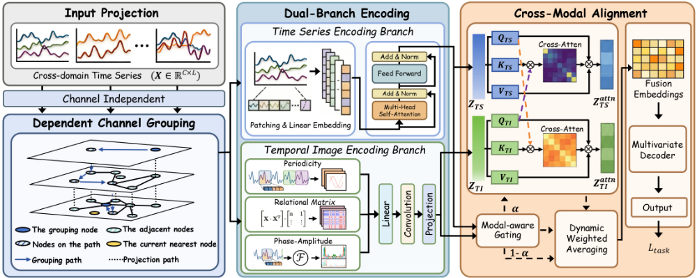
Figure 1 shows the framework overview of the proposed TimeIG. As shown in the figure, TimeIG consists of four major modules: Input Projection, Dependent Channel Grouping, Dual-Branch Encoding, and Cross-Modal Alignment. Specifically, Dependent Channel Grouping selects K anchor channels to align varying dimensions into a standardized latent space. Next, Dual-Branch Encoding captures multifaceted features through two parallel branches. Time Series Encoding branch directly encodes the temporal numerical information, while the tailored Temporal Imaging Encoding branch extracts structural correlations by transforming sequences into visual data. Finally, Cross-Modal Alignment adaptively fuses these representations using Cross-Modal Attention (CMAM) and Dynamic Weighted-Averaging (DWAM) to form a unified representation. Next, we provide the technical details of each module, respectively.
integrated via a distance-weighted fusion mechanism. Specifically, first, feature channels are randomly selected, and then the newly added features are connected to the existing features, performing a hierarchical projection. Each channel's time series is mapped onto the closest representative channels weighted inversely by their distance:
where xj is the time series of the channel j, d(·, ·) is a distance metric between time series, and x′j is the fused representation obtained by weighted aggregation. This weighted fusion ensures that the discarded features' information is not completely lost, but softly integrated into the lowdimensional feature space via their nearest representative channels. Through the above procedure, a fixed dimension K representation of the multivariate time series is obtained, preserving the majority of the original variables' information and structural characteristics. Leveraging this structure for nearest neighbor grouping on this reduced space further ensures efficient and effective similarity queries.
3.3 Dual-Branch Encoding
To capture the multifaceted dependencies within the standardized K-dimensional representation X ∈ RB×K×T , we propose a dual-branch encoding module. As shown in the central part of Figure 1 , this module independently models time series encoding branch and temporal image encoding branch, facilitating a comprehensive understanding of complex time series patterns.
Time Series Encoding Branch. Time series encoding branch aims to capture long-range temporal dependencies within a unified, standardized space. Unlike task-specific models that rely on isolated local patterns, our approach employs a Multi-Head Self-Attention (MHSA) mechanism to model the global dynamics of the input patch sequence.
3.1 Input Projection
In this paper, we define the cross-domain datasets as D = {D1,D2, . . . ,DN}, where each domain Di contains multiple time series Di = {T i 1 , T i 2 , . . . , T ini } ∈ RC×L, where C denotes the number of channels and L denotes the length, which together lead to the cross-domain data being heterogeneous. We regard each time series as a channel, and the relationships between different channels are crucial for crossdomain time series models. Most existing studies [Liu et al., 2024c] employ channel-independence mechanisms to accommodate cross-domain time series with different dimensionalities, which ignores the correlations across channels. In contrast, we adopt channel mixing to capture cross-variable interactions and extract more comprehensive temporal patterns. Initially, the original C-dimensional multivariate time series is decomposed into C one-dimensional time series via channel independent processing.
3.2 Dependent Channel Grouping
As shown in the left part of Figure 1, in the dimensionality reduction and fusion process of multivariate time series, we propose a distance-weighted representative feature selection mechanism via Dependent Channel Grouping. To achieve the target of fixed-dimensionality reduction, a subset of K < C most representative time series channels is selected from the channels processed by channel-independent handling as core features. This selection aims to retain the subset with the maximal information content and expressive power among the multivariate data. The selection of the K most influential anchor channels, denoted by the set S, is formulated as an optimization problem:
where R(i) denotes the representativeness score of channel i. For the remaining (N -K) channels, their information is Given the sequence of patches (where M is the total number of patches), the updated temporal representation H is computed as:
where Q,K,V ∈ RM×d are the query, key, and value matrices projected from the complete set of M patches, d is the hidden dimension, dk is the dimension of the key vectors. This global attention mechanism enables the model to perceive dependencies across the entire temporal horizon. To align these sequential features with our group-wise modeling strategy, we introduce a learnable aggregation operator A. This operator distills the high-dimensional temporal information into group-specific features ZTS:
where K denotes the number of dependent channel groups, B is the batch size. This formulation ensures that the learned temporal evolution is both robust and consistent with the cross-modal grouping logic, facilitating a task-aware representation that transcends individual channel variations.
Temporal Image Encoding Branch. To complement the temporal encoding, the temporal imaging encoding branch characterizes the structural interactions among variables by mapping the sequence into a visual modality I ∈ RB×L×K×C . We define a multi-view decomposition operator Ψ that extracts features through three parallel streams reflecting fundamental mathematical properties of the data:
- Periodicity: To capture the multi-scale rhythmicity inherent in complex time series, the operator Hper employs temporal convolutions to discern recurrent motifs and cyclical oscillations. This process yields Zper = Hper(X) ∈ RB×L×K×2 , which encodes the local and global temporal regularities.
- Relational Matrix: Addressing the latent topological dependencies across variables, the spatial operator Hrel computes a dynamic correlation graph. This stream facilitates the modeling of inter-variable synergies, represented as Zrel = Hrel(X) ∈ RB×L×K×1 , providing a structural blueprint of the system's internal interactions.
- Phase-Amplitude: Recognizing that temporal dynamics are often governed by spectral properties, the frequency-domain operator Hfreq decomposes the signal into learned spectral bases. By extracting the phase and amplitude characteristics, it generates Zfreq = Hfreq(X) ∈ RB×L×K×2 , capturing the energy distribution of the signal across the frequency spectrum.
The resulting multi-view descriptors are integrated into a cohesive structural representation ZTI through a synergistic fusion sequence. By employing a channel-wise concatenation followed by a learnable convolutional projection, the model distills the heterogeneous perspectives into a compact structural fingerprint:
Where d′ is the projected feature dimension By explicitly decoupling temporal evolution from cross-variable structural correlations, this branch effectively mitigates the representational bottlenecks inherent in purely sequential architectures and enhances the model's inductive bias toward complex data patterns.
3.4 Cross-Modal Alignment
Following the extraction of decoupled features from the two branches, the framework must synergistically integrate these representations to form a comprehensive embedding. As shown in the right part of Figure 1, we propose an adaptive alignment module consisting of a Cross-Modal Attention Mechanism (CMAM) and a Dynamic Weighted-Averaging Mechanism (DWAM) to achieve optimal feature synthesis based on input-specific characteristics.
Cross-Modal Attention Mechanism. To emphasize complementary information while suppressing modality-specific redundancy, CMAM leverages a dual-stream attention operator to model the latent interactions between temporal evolution ZTS and structural correlations ZTI. We first project these features into a shared latent space via linear transformations ϕTS and ϕTI. The cross-modal interaction is formulated through the Query (Q), Key (K), and Value (V) paradigm:
where the query of one modality retrieves relevant structural or temporal contexts from the other. This bi-directional flow ensures that the fused representation preserves the intrinsic temporal-spatial duality of the data.
Dynamic Weighted-Averaging Mechanism. Since the contribution of each modality varies across different samples and tasks, we introduce DWAM to adaptively determine the fusion intensity. We define a learnable gating function Gθ parameterized by a lightweight multilayer perceptron (MLP). The dynamic weight α is estimated by jointly considering the concatenated global features:
where ⊕ denotes the concatenation operator and σ represents the sigmoid activation. The final fused embedding Ffusion is synthesized as a convex combination of the attentive features:
This mechanism facilitates a sample-wise weighting strategy, enabling the framework to flexibly prioritize either sequential dynamics or structural relationships depending on the input's complexity.
Multivariate Decoder. The fused representation Ffusion is subsequently fed into a multivariate Transformer decoder specialized for task-specific inference. By modeling the longrange dependencies embedded in the synthesized features, the decoder generates the final output Y for various analytical tasks:
| Models | ETTm1 | ETTm2 | ETTh1 | ETTh2 | ECL | Weather | Traffic | Solar | ||||||||
|---|---|---|---|---|---|---|---|---|---|---|---|---|---|---|---|---|
| MSE | MAE | MSE | MAE | MSE | MAE | MSE | MAE | MSE | MAE | MSE | MAE | MSE | MAE | MSE | MAE | |
| ARIMA | 1.172 | 0.813 | 2.425 | 1.208 | 1.228 | 0.851 | 3.126 | 1.382 | 0.589 | 0.579 | 0.474 | 0.484 | 1.041 | 0.572 | 1.293 | 1.375 |
| N-HiTS | 0.452 | 0.461 | 0.305 | 0.370 | 0.493 | 0.514 | 0.436 | 0.470 | 0.210 | 0.313 | 0.279 | 0.317 | 0.457 | 0.344 | 0.285 | 0.307 |
| TimesNet | 0.525 | 0.521 | 0.411 | 0.453 | 0.578 | 0.570 | 0.527 | 0.547 | 0.231 | 0.333 | 0.294 | 0.323 | 0.632 | 0.352 | 0.243 | 0.325 |
| PatchTST | 0.439 | 0.460 | 0.361 | 0.411 | 0.480 | 0.502 | 0.393 | 0.405 | 0.199 | 0.298 | 0.257 | 0.298 | 0.421 | 0.305 | 0.232 | 0.299 |
| DLinear | 0.453 | 0.467 | 0.461 | 0.477 | 0.473 | 0.479 | 0.376 | 0.432 | 0.195 | 0.295 | 0.270 | 0.321 | 0.453 | 0.328 | 0.252 | 0.313 |
| UniTime | 0.419 | 0.626 | 0.470 | 0.494 | 0.634 | 0.623 | 0.555 | 0.563 | 0.189 | 0.429 | 0.265 | 0.489 | 0.404 | 0.397 | 0.227 | 0.492 |
| TimeVLM | 0.371 | 0.410 | 0.289 | 0.355 | 0.440 | 0.451 | 0.364 | 0.410 | 0.190 | 0.294 | 0.257 | 0.296 | 0.463 | 0.341 | 0.247 | 0.297 |
| iTransformer | 0.428 | 0.436 | 0.316 | 0.358 | 0.466 | 0.487 | 0.412 | 0.445 | 0.197 | 0.286 | 0.289 | 0.306 | 0.460 | 0.305 | 0.269 | 0.290 |
| UniTS | 0.459 | 0.469 | 0.478 | 0.494 | 0.474 | 0.426 | 0.384 | 0.379 | 0.214 | 0.312 | 0.258 | 0.298 | 0.491 | 0.356 | 0.266 | 0.333 |
| AutoTimes | 0.438 | 0.452 | 0.453 | 0.511 | 0.617 | 0.640 | 0.538 | 0.580 | 0.355 | 0.283 | 0.491 | 0.303 | 0.614 | 0.369 | 0.422 | 0.272 |
| TimeLLM | 0.442 | 0.467 | 0.493 | 0.526 | 0.657 | 0.655 | 0.578 | 0.595 | 0.211 | 0.318 | 0.255 | 0.295 | 0.440 | 0.333 | 0.293 | 0.365 |
| Timer | 0.384 | 0.418 | 0.295 | 0.354 | 0.420 | 0.448 | 0.370 | 0.417 | 0.199 | 0.295 | 0.263 | 0.301 | 0.291 | 0.248 | 0.352 | 0.422 |
| TimerXL | 0.366 | 0.407 | 0.288 | 0.350 | 0.441 | 0.464 | 0.363 | 0.417 | 0.199 | 0.295 | 0.264 | 0.300 | 0.307 | 0.255 | 0.223 | 0.295 |
| TimeIG | 0.356 | 0.393 | 0.258 | 0.320 | 0.395 | 0.419 | 0.340 | 0.390 | 0.182 | 0.262 | 0.242 | 0.284 | 0.314 | 0.259 | 0.192 | 0.203 |
where Gϕ represents the task-specific projection head optimized to minimize independent loss objectives L(t) .
3.5 Pre-training and Fine-tuning
Pre-training. The goal of the pre-trained model MΘ is to learn general cross-domain feature representations. For this purpose, we design the objective function as follows:
where z(·;Θ) represents the feature vector representation of a time series, zavg is the average of all domain features, and λ is a weighting coefficient that balances the generation probability and feature consistency. By independently optimizing θt for each task, the framework maintains specialization and high performance tailored to each task's data characteristics and objectives. Meanwhile, the shared multi-modal architecture fosters parameter and representation reuse, enabling effective transfer and robustness in cross-domain, multi-task time series applications. Existing time series foundation models[Liu et al., 2024g; Gao et al., 2024] show that pretraining enhances the model performance since more training data is involved, introducing more useful knowledge. Motivated by this, we pre-train TimeIG with the UTSD4G dataset[Liu et al., 2024g] and then finetune it for new datasets.
Fine-tuning. This work proposes a unified cross-modal framework designed to support multiple heterogeneous time series tasks, including prediction, classification, and anomaly detection. Although the framework enables a shared representation and fusion mechanism across tasks and domains, each task's model parameters θt are optimized independently to accommodate their distinct objectives and data distributions.
Formally, for each task t, given its corresponding dataset Dt = {(X(t) i , y(t) i )}Nt i=1 , the training objective is to minimize the task-specific loss:
where fθt (·) denotes the model inference for task t. In crossdomain time-series analysis, a cross-domain dataset is defined as D = {D1,D2, . . . ,DN}, where each domain Di contains multiple time series Di = {T i 1 , T i 2 , . . . , T ini }.
4 Experiments
In this section, we systematically evaluate the efficacy of TimeIG across various tasks within the time series domain, complemented by ablation experiments that elucidate the individual contributions of its components to the overall performance (refer to Section 4.5). To rigorously assess the generalizability of the TimeIG approach, we conduct extensive empirical analyses across three critical time series tasks: Time Series Forecasting (see Table 1), Anomaly Detection (see Table 2), and Classification (see Table 3).
4.1 Datasets and Experiment Setup
Datasets. The experiments are carried out on certain realworld time series datasets. In terms of forecasting, we employ 8 datasets, including ETTh1, ETTh2, ETTm1, ETTm2, ECL, Trafffc, Weather [Wu et al., 2021], and Solar [Liu et al., 2024d]. For anomaly detection, we adopt 5 datasets,including SMD, PSM, SWaT, MSL, and SMAP [Liu et al., 2024a]. For time series classification, we employ UEA [Bagnall et al., 2018].
Baselines. We compare TimeIG with the following existing baselines, including 13 time series forecasting baselines, i.e., ARIMA [Stellwagen and Tashman, 2013], DLinear [Zeng et al., 2021] TimesNet [Wu et al., 2023], PatchTST [Nie et al., 2023], N-HiTS [Challu et al., 2023], iTransformer [Liu et al., 2024e], TimeVLM [Zhong et al., 2025], TimeLLM [Jin et al., 2024], AutoTimes [Liu et al., 2024f], UniTime [Liu et al., 2024c], UniTS [Gao et al., 2024], Timer [Liu et al., 2024g], and TimerXL [Liu et al., 2025c]. For anomaly detection, we compare TimeIG with ARIMA [Stellwagen and Tashman,
| Models | SMD | PSM | SWaT | MSL | SMAP | Average | ||||||||||||
|---|---|---|---|---|---|---|---|---|---|---|---|---|---|---|---|---|---|---|
| F1 | AUC | PATE | F1 | AUC | PATE | F1 | AUC | PATE | F1 | AUC | PATE | F1 | AUC | PATE | F1 | AUC | PATE | |
| ARIMA | 31.74 | 26.95 | 13.59 | 36.21 | 31.25 | 42.13 | 32.99 | 34.98 | 11.59 | 26.95 | 29.99 | 16.39 | 24.69 | 27.10 | 16.98 | 30.52 | 30.05 | 20.14 |
| FEDformer | 75.63 | 68.32 | 57.90 | 70.31 | 78.45 | 55.34 | 52.36 | 59.48 | 43.63 | 48.69 | 50.98 | 65.32 | 51.46 | 69.47 | 48.01 | 59.69 | 65.34 | 54.04 |
| Informer | 69.35 | 82.48 | 67.49 | 65.20 | 74.32 | 57.64 | 33.65 | 54.31 | 23.31 | 66.54 | 78.31 | 77.31 | 76.86 | 63.73 | 64.85 | 62.32 | 70.63 | 58.12 |
| DCdetector | 65.48 | 80.36 | 68.93 | 60.38 | 68.32 | 51.36 | 68.36 | 62.31 | 67.41 | 56.70 | 66.54 | 56.30 | 23.88 | 60.07 | 40.80 | 54.96 | 67.52 | 56.96 |
| Autoformer | 57.90 | 58.69 | 62.47 | 59.58 | 68.75 | 65.30 | 67.54 | 56.63 | 65.25 | 44.68 | 59.62 | 66.75 | 40.40 | 57.46 | 46.73 | 54.02 | 60.23 | 61.30 |
| DLinear | 68.49 | 74.75 | 55.46 | 70.65 | 76.49 | 43.59 | 60.70 | 70.53 | 56.78 | 65.31 | 69.49 | 58.61 | 66.75 | 68.84 | 55.16 | 66.38 | 72.02 | 53.92 |
| TimesNet | 69.74 | 73.85 | 64.90 | 73.21 | 75.65 | 72.60 | 65.19 | 68.93 | 58.36 | 75.36 | 77.69 | 85.36 | 67.15 | 69.98 | 73.83 | 70.13 | 73.22 | 71.01 |
| Ser2graph | 63.51 | 71.65 | 55.32 | 64.98 | 69.46 | 66.79 | 56.84 | 66.32 | 59.64 | 59.64 | 68.49 | 55.30 | 66.70 | 68.31 | 59.67 | 62.33 | 68.85 | 59.34 |
| TranAD | 66.31 | 75.65 | 62.98 | 65.39 | 71.85 | 67.59 | 64.25 | 71.36 | 62.39 | 63.59 | 69.75 | 62.98 | 59.62 | 65.31 | 60.81 | 63.83 | 70.78 | 63.35 |
| IMDIFFUSION | 69.75 | 73.86 | 64.91 | 73.32 | 75.76 | 72.71 | 65.20 | 75.65 | 75.36 | 75.37 | 77.70 | 85.37 | 67.16 | 69.99 | 73.84 | 70.16 | 74.59 | 74.44 |
| Timer | 79.65 | 82.36 | 61.87 | 80.02 | 83.54 | 62.39 | 77.06 | 79.65 | 58.67 | 75.09 | 75.63 | 57.31 | 77.63 | 77.17 | 60.81 | 77.89 | 79.67 | 60.21 |
| TimeIG | 82.61 | 85.96 | 77.31 | 83.26 | 85.64 | 76.59 | 79.67 | 85.95 | 72.69 | 74.62 | 85.45 | 79.56 | 80.06 | 83.55 | 72.50 | 80.52 | 85.31 | 75.73 |
2013], FEDformer [Zhou et al., 2022], Informer [Zhou et al., 2021], DCdetector [Yang et al., 2023], Autoformer [Wu et al., 2021], DLinear [Zeng et al., 2021], TimesNet [Wu et al., 2023], Series2graph (Ser2graph) [Paul Boniol, 2020], TranAD [Shreshth Tuli, 2022], IMDIFFUSION [Chen et al., 2023] and Timer [Liu et al., 2024g]. For time series classification, 13 baselines are selected, i.e., LSTM [Shi et al., 2015], LSTNET [Lai et al., 2018], Informer [Zhou et al., 2021], FEDformer [Zhou et al., 2022], Full Attention (Attn) [Haoqing Wang, 2023], [Dempster et al., 2020], InceptionTime [Ismail Fawaz et al., 2020], TCN [Bai et al., 2018], LIGHTTS [Campos et al., 2023], DLinear [Zeng et al., 2021], TimesNet [Wu et al., 2023], UniTS [Gao et al., 2024], and Timer [Liu et al., 2024g]. Please note that TimeLLM is a large language mode based time series analytics method, while Timer, TimerXL, and UniTS are time series foundation models. We follow the default hyperparameter setting in the original paper or the associated code of baselines, enabling fair comparison.
Evaluation Metrics. We adopt mean squared error (MSE) and mean absolute error (MAE) as evaluation metrics for time series forecasting [Qiu et al., 2024]. The F1-score (F1), AUCROC, and PATE [Ghorbani et al., 2024] are adopted as main evaluation metrics for time series anomaly detection. Additionally, F1 and accuracy are used to evaluate time series classification.
4.2 Time Series Forecasting
Time series forecasting is a central task. We evaluate TimeIG against 13 baselines on standard benchmarks (ETTh, ECL, Weather, Traffic, Solar). Time series foundation models (TimeIG, Timer, TimeXL, UniTS) are trained and tested simultaneously on all datasets. As shown in Table 1, TimeIG achieves the best performance in most cases across prediction lengths from 96 to 720, outperforming the best baseline by up to 15.9%. ARIMA performs worst, as traditional statistics-based methods are shallow and fail to capture complex temporal correlations. Moreover, time series foundation models generally outperform both transformer-based (e.g., PatchTST) and MLP-based (e.g., TimesNet) methods, demonstrating their superior generalization capabilities.
4.3 Anomaly Detection
Since the anomalies are usually hidden in the large-scale data, making the data labeling hard, we focus on unsupervised time series anomaly detection, which is to detect the abnormal time points. We evaluate unsupervised point-wise anomaly detection on five benchmarks (SMD, MSL, SMAP, SWaT, PSM) spanning service monitoring, space telemetry, and industrial control. Following Anomaly Transformer, we use fixed-length sliding windows and train via reconstruction. We report F1, AUC, and PATE as our primary metrics as prior works [Ghorbani et al., 2024; Liu et al., 2024a].
As shown in Table 2, TimeIG attains the highest average performance across five benchmarks on F1/AUC/PATE (80.20/85.31/75.73). It ranks first on SMD and PSM across all three metrics; on SMD, TimeIG reaches 12.4% absolute gain in terms of PATE over the second-best IMDIFFICTION. These results demonstrate that TimeIG provides stable crossdomain generalization and effective range handling in unsupervised anomaly detection.
4.4 Classification
| Models | Accuracy | F1 | R | AUC |
|---|---|---|---|---|
| Informer | 0.678 | 0.662 | 0.632 | 0.659 |
| FEDformer | 0.729 | 0.634 | 0.696 | 0.682 |
| Full Attn | 0.721 | 0.688 | 0.684 | 0.677 |
| LIGHTTS | 0.702 | 0.674 | 0.711 | 0.666 |
| DLinear | 0.736 | 0.709 | 0.701 | 0.677 |
| LSTM | 0.521 | 0.569 | 0.598 | 0.519 |
| LSTNET | 0.663 | 0.658 | 0.685 | 0.649 |
| TimesNet | 0.740 | 0.717 | 0.698 | 0.686 |
| UniTS | 0.726 | 0.693 | 0.696 | 0.679 |
| Rocket | 0.753 | 0.719 | 0.701 | 0.684 |
| InceptionTime | 0.712 | 0.688 | 0.700 | 0.685 |
| TCN | 0.700 | 0.675 | 0.695 | 0.675 |
| Timer | 0.752 | 0.718 | 0.703 | 0.696 |
| TimeIG | 0.762 | 0.723 | 0.713 | 0.687 |
We conduct time series classification experiments on 10 UEA subsets using Accuracy and F1-score. The overall average results are in Table 3. TimeIG outperforms all baselines and achieves the best results on all 10 datasets, demonstrating its effectiveness. Among baselines, the foundation model Timer achieves the best performance, surpassing the previous SOTA by 1.4% and 0.6%, highlighting the potential of foundation models. TimeIG improves over Timer due to its dual-branch encoding module, which learns effective representations across two complementary modalities. This dualbranch approach enhances feature extraction and provides a more robust classification framework by integrating diverse information sources. The comparative analysis in Table 3 further confirms TimeIG's superior accuracy and F1-score, underscoring its adaptability and reliability on complex time series data.
w/o_CMA TimeIG
(a) ECL
w/o_CMA TimeIG
(b) Traffic
4.5 Ablation Study
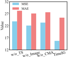
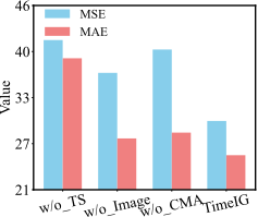
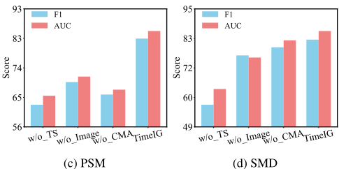
To understand the effects of TimeIG's different components, we evaluate three components: 1) w/o TS: TimeIG without time series encoding branch; 2) w/o Image: TimeIG without time image encoding branch; 3) w/o CMA: TimeIG without cross-modal attention mechanism. Figure 2 shows results for forecasting (a,b) and anomaly detection (c,d). Regardless of the datasets, TimeIG outperforms its counterparts, showing that these three components are all useful for effective universal time series modeling. TimeIG obtains MSE and MAE reductions up to 38.6% and 22.5%. Further, on all datasets, w/o TS performs worst among all variants. TimeIG performs better than w/o TS by at least 8%, which indicates the importance of time series encoding branch.
4.6 Case Study
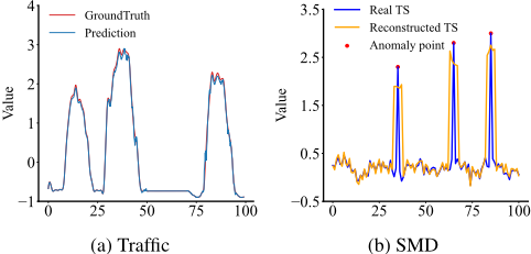
To intuitively show the effectiveness of the proposed TimeIG, we provide case studies on Traffic and SMD in terms of forecasting and anomaly detection, respectively, as shown in Figure 3. In Figure 3(a), we see that the predictions are highly consistent with the ground truth, demonstrating the effectiveness of TimeIG. Figure 3(b) shows that TimeIG successfully identifies the outliers on SMD, demonstrating its superior performance for anomaly detection. These two figures jointly demonstrate that the TimeIG model can accurately predict future trends and promptly detect anomalies when handling different time series analysis tasks.
4.7 The Effect of Hyper-parameter K
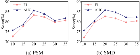
We next investigate the effect of the number of K on model performance, which denotes the number of selected representative channels. We vary K within the range of {10, 15, 20, 25, 30, 35} to evaluate its sensitivity. As shown in Figure 4, we observe that the F1 and AUC curves first increase, then drop, and finally increase slightly. TimeIG achieves the best performance when K is set to 20, which shows that 20 is the ideal setting in this study. While a larger K increases data coverage, excessive channels introduce noise and redundancy, hindering cross-modal alignment and degrading task generalization.
5 Conclusion
This work presents TimeIG, a modality-aware dual-branch framework for universal time series analysis. To handle heterogeneous dimensionalities, we propose a channel dependency search to select representative channels. For comprehensive feature extraction, we introduce a time series imaging method and a dual-branch architecture for joint sequence and vision representation learning, along with a cross-modal alignment module to fuse complementary features. Extensive experiments show TimeIG achieves state-of-the-art accuracy.
Acknowledgments
This work is partially supported by the National Natural Science Foundation of China (No.62572489) and SCRI, The Hong Kong Polytechnic University (No. Q-CDDG).
Contribution Statement
Minjun Cao and Hao Miao are co-first authors with equal contributions. Senzhang Wang is the corresponding author.
@inproceedings{ijcai2026p272,
  title     = {From Diversity to Uniformity: Cross-modal Time Series Modeling with Dependent Channel Grouping},
  author    = {Cao, Minjun and Miao, Hao and Zhang, Wentao and Wang, Senzhang},
  booktitle = {Proceedings of the Thirty-Fifth International Joint Conference on
               Artificial Intelligence, {IJCAI-26}},
  publisher = {International Joint Conferences on Artificial Intelligence Organization},
  editor    = {Diego Calvanese},
  pages     = {2447--2455},
  year      = {2026},
  month     = {8},
  note      = {Main Track},
  doi       = {10.24963/ijcai.2026/272},
  url       = {https://doi.org/10.24963/ijcai.2026/272},
}
TY - CPAPER TI - From Diversity to Uniformity: Cross-modal Time Series Modeling with Dependent Channel Grouping AU - Cao, Minjun AU - Miao, Hao AU - Zhang, Wentao AU - Wang, Senzhang T2 - Proceedings of the Thirty-Fifth International Joint Conference on Artificial Intelligence, IJCAI-26 PB - International Joint Conferences on Artificial Intelligence Organization PY - 2026 SP - 2447 EP - 2455 DO - 10.24963/ijcai.2026/272 UR - https://doi.org/10.24963/ijcai.2026/272 ER -Copied
Machine-readable versions of this paper, for tools and AI agents:





