
DiSGMM: A Method for Time-varying Microscopic Weight Completion on Road Networks
Proceedings of the Thirty-Fifth International Joint Conference on Artificial Intelligence. Main Track. Pages 2834-2842.
https://doi.org/10.24963/ijcai.2026/315
Keywords
- Data Mining: Mining spatial and/or temporal data
- Multidisciplinary Topics and Applications: Transportation
Abstract
Microscopic road-network weights represent fine-grained, time-varying traffic conditions obtained from individual vehicles. An example is travel speeds associated with road segments as vehicles traverse them. These weights support tasks including traffic microsimulation and vehicle routing with reliability guarantees.
We study the problem of time-varying microscopic weight completion. During a time slot, the available weights typically cover only some road segments. Weight completion recovers distributions for the weights of every road segment at the current time slot.
This problem involves two challenges: (i) contending with two layers of sparsity, where weights are missing at both the network layer (many road segments lack weights) and the segment layer (a segment may have insufficient weights to enable accurate distribution estimation); and (ii) achieving a weight distribution representation that is closed-form and can capture complex conditions flexibly, including heavy tails and multiple clusters.
To address these challenges, we propose DiSGMM that combines sparsity-aware embeddings with spatiotemporal modeling to leverage sparse known weights alongside learned segment properties and long-range correlations for distribution estimation. DiSGMM represents distributions of microscopic weights as learnable Gaussian mixture models, providing closed-form distributions capable of capturing complex conditions flexibly. Experiments on two real-world datasets show that DiSGMM can outperform state-of-the-art methods.
- [Abou Elassad et al., 2020] Zouhair Elamrani Abou Elassad, Hajar Mousannif, Hassan Al Moatassime, and Aimad Karkouch. The application of machine learning techniques for driving behavior analysis: A conceptual framework and a systematic literature review. Eng. Appl. Artif. Intell., 87:103312, 2020.
- [Akhtar and Moridpour, 2021] Mahmuda Akhtar and Sara Moridpour. A review of traffic congestion prediction using artificial intelligence. J. Adv. Transp., 2021(1):8878011, 2021.
- [An et al., 2024] Yang An, Zhibin Li, Wei Liu, Haoliang Sun, Meng Chen, Wenpeng Lu, and Yongshun Gong. Spatio-temporal graph normalizing flow for probabilistic traffic prediction. In CIKM, pages 45-55, 2024.
- [Blondel et al., 2008] Vincent D Blondel, Jean-Loup Guil- laume, Renaud Lambiotte, and Etienne Lefebvre. Fast un- folding of communities in large networks. J. Stat. Mech. Theory Exp., 2008(10):P10008, 2008.
- [Cao et al., 2018] Wei Cao, Dong Wang, Jian Li, Hao Zhou, Lei Li, and Yitan Li. BRITS: bidirectional recurrent im- putation for time series. In NeurIPS, pages 6776-6786, 2018.
- [Chen et al., 2022] Xinyu Chen, Mengying Lei, Nicolas Saunier, and Lijun Sun. Low-rank autoregressive ten- sor completion for spatiotemporal traffic data imputation. IEEE Trans. Intell. Transp. Syst., 23(8):12301-12310, 2022.
- [Chung et al., 2014] Junyoung Chung, Caglar Gulcehre, KyungHyun Cho, and Yoshua Bengio. Empirical evalua- tion of gated recurrent neural networks on sequence mod- eling. arXiv preprint arXiv:1412.3555, 2014.
- [Cini et al., 2022] Andrea Cini, Ivan Marisca, and Cesare Alippi. Filling the g ap s: Multivariate time series im- putation by graph neural networks. In ICLR, 2022.
- [Fang et al., 2022] Ziquan Fang, Yuntao Du, Xinjun Zhu, Danlei Hu, Lu Chen, Yunjun Gao, and Christian S. Jensen. Spatio-temporal trajectory similarity learning in road net- works. In SIGKDD, pages 347-356, 2022.
- [Gao et al., 2015] Yunjun Gao, Xu Qin, Baihua Zheng, and Gang Chen. Efficient reverse top-k boolean spatial key- word queries on road networks. IEEE Trans. Knowl. Data Eng., 27(5):1205-1218, 2015.
- [Goodfellow et al., 2014] Ian J. Goodfellow, Jean Pouget- Abadie, Mehdi Mirza, Bing Xu, David Warde-Farley, Sherjil Ozair, Aaron C. Courville, and Yoshua Bengio. Generative adversarial nets. In NeurIPS, pages 2672- 2680, 2014.
- [Guo et al., 2019] Shengnan Guo, Youfang Lin, Ning Feng, Chao Song, and Huaiyu Wan. Attention based spatial- temporal graph convolutional networks for traffic flow forecasting. In AAAI, pages 922-929, 2019.
- [Han et al., 2022] Xiaolin Han, Reynold Cheng, Tobias Grubenmann, Silviu Maniu, Chenhao Ma, and Xiaodong Li. Leveraging contextual graphs for stochastic weight completion in sparse road networks. In SDM, pages 64-72, 2022.
- [Ho et al., 2020a] Jonathan Ho, Ajay Jain, and Pieter Abbeel. Denoising diffusion probabilistic models. NeurIPS, 33:6840-6851, 2020.
- [Ho et al., 2020b] Jonathan Ho, Ajay Jain, and Pieter Abbeel. Denoising diffusion probabilistic models. In NeurIPS, 2020.
- [Hochreiter and Schmidhuber, 1997] Sepp Hochreiter and Jürgen Schmidhuber. Long short-term memory. Neural Comput., 9(8):1735-1780, 1997.
- [Hollander and Liu, 2008] Yaron Hollander and Ronghui Liu. The principles of calibrating traffic microsimulation models. Transportation, 35(3):347-362, 2008.
- [Hu et al., 2019] Jilin Hu, Chenjuan Guo, Bin Yang, and Christian S. Jensen. Stochastic weight completion for road networks using graph convolutional networks. In ICDE, pages 1274-1285, 2019.
- [Jiang and Luo, 2022] Weiwei Jiang and Jiayun Luo. Graph neural network for traffic forecasting: A survey. Expert Syst. Appl., 207:117921, 2022.
- [Jin et al., 2023] Guangyin Jin, Yuxuan Liang, Yuchen Fang, Zezhi Shao, Jincai Huang, Junbo Zhang, and Yu Zheng. Spatio-temporal graph neural networks for predictive learning in urban computing: A survey. IEEE Trans. Knowl. Data Eng., 36(10):5388-5408, 2023.
- [Kipf and Welling, 2017] Thomas N. Kipf and Max Welling. Semi-supervised classification with graph convolutional networks. In ICLR, 2017.
- [Lea et al., 2016] Colin Lea, Rene Vidal, Austin Reiter, and Gregory D Hager. Temporal convolutional networks: A unified approach to action segmentation. In ECCV, pages 47-54, 2016.
- [Li et al., 2019] Steven Cheng-Xian Li, Bo Jiang, and Ben- jamin M. Marlin. Misgan: Learning from incomplete data with generative adversarial networks. In ICLR, 2019.
- [Li et al., 2021] Yang Li, Si Si, Gang Li, Cho-Jui Hsieh, and Samy Bengio. Learnable fourier features for multi- dimensional spatial positional encoding. In NeurIPS, pages 15816-15829, 2021.
- [Liu et al., 2019] Yukai Liu, Rose Yu, Stephan Zheng, Eric Zhan, and Yisong Yue. NAOMI: non-autoregressive mul- tiresolution sequence imputation. In NeurIPS, pages 11236-11246, 2019.
- [Liu et al., 2023] Mingzhe Liu, Han Huang, Hao Feng, Leilei Sun, Bowen Du, and Yanjie Fu. Pristi: A condi- tional diffusion framework for spatiotemporal imputation. In ICDE, pages 1927-1939, 2023.
- [Matheson and Winkler, 1976] James E Matheson and Robert L Winkler. Scoring rules for continuous prob- ability distributions. Manag. Sci., 22(10):1087-1096, 1976.
- [Mikolov et al., 2013] Tomás Mikolov, Kai Chen, Greg Cor- rado, and Jeffrey Dean. Efficient estimation of word rep- resentations in vector space. In ICLR, 2013.
- [Muñiz-Cuza et al., 2022] Carlos Enrique Muñiz-Cuza, Nguyen Ho, Eleni Tzirita Zacharatou, Torben Bach Pedersen, and Bin Yang. Spatio-temporal graph convolu- tional network for stochastic traffic speed imputation. In SIGSPATIAL, pages 14:1-14:12, 2022.
- [Nie et al., 2024] Tong Nie, Guoyang Qin, Wei Ma, Yuewen Mei, and Jian Sun. Imputeformer: Low rankness-induced transformers for generalizable spatiotemporal imputation. In SIGKDD, pages 2260-2271, 2024.
- [Paszke et al., 2019] Adam Paszke, Sam Gross, Francisco Massa, Adam Lerer, James Bradbury, Gregory Chanan, Trevor Killeen, Zeming Lin, Natalia Gimelshein, Luca Antiga, Alban Desmaison, Andreas Köpf, Edward Z. Yang, Zachary DeVito, Martin Raison, Alykhan Tejani, Sasank Chilamkurthy, Benoit Steiner, Lu Fang, Junjie Bai, and Soumith Chintala. Pytorch: An imperative style, high- performance deep learning library. In NeurIPS, pages 8024-8035, 2019.
- [Perozzi et al., 2014] Bryan Perozzi, Rami Al-Rfou, and Steven Skiena. Deepwalk: online learning of social rep- resentations. In SIGKDD, pages 701-710, 2014.
- [Reynolds and others, 2009] Douglas A Reynolds et al. Gaussian mixture models. Encyclopedia of biometrics, 741(659-663), 2009.
- [Ronneberger et al., 2015] Olaf Ronneberger, Philipp Fis- cher, and Thomas Brox. U-net: Convolutional networks for biomedical image segmentation. In MICCAI, volume 9351, pages 234-241, 2015.
- [Shao, 2003] Jun Shao. Mathematical statistics. Springer Science & Business Media, 2003.
- [Shukla and Marlin, 2021] Satya Narayan Shukla and Ben- jamin M. Marlin. Multi-time attention networks for irreg- ularly sampled time series. In ICLR, 2021.
- [Song et al., 2019] Qingquan Song, Hancheng Ge, James Caverlee, and Xia Hu. Tensor completion algorithms in big data analytics. ACM Trans. Knowl. Discov. Data, 13(1):6:1-6:48, 2019.
- [Tashiro et al., 2021] Yusuke Tashiro, Jiaming Song, Yang Song, and Stefano Ermon. CSDI: conditional score-based diffusion models for probabilistic time series imputation. In NeurIPS, pages 24804-24816, 2021.
- [Tedjopurnomo et al., 2020] David Alexander Tedjop- urnomo, Zhifeng Bao, Baihua Zheng, Farhana Murtaza Choudhury, and Alex Kai Qin. A survey on modern deep neural network for traffic prediction: Trends, meth- ods and challenges. IEEE Trans. Knowl. Data Eng., 34(4):1544-1561, 2020.
- [Vaswani et al., 2017] Ashish Vaswani, Noam Shazeer, Niki Parmar, Jakob Uszkoreit, Llion Jones, Aidan N. Gomez, Lukasz Kaiser, and Illia Polosukhin. Attention is all you need. In NeurIPS, pages 5998-6008, 2017.
- [Wei et al., 2024] Tonglong Wei, Youfang Lin, Shengnan Guo, Yan Lin, Yiji Zhao, Xiyuan Jin, Zhihao Wu, and Huaiyu Wan. Inductive and adaptive graph convolu- tion networks equipped with constraint task for spatial- temporal traffic data kriging. Knowl. Based Syst., 284:111325, 2024.
- [Wen et al., 2023a] Haomin Wen, Youfang Lin, Yutong Xia, Huaiyu Wan, Qingsong Wen, Roger Zimmermann, and Yuxuan Liang. Diffstg: Probabilistic spatio-temporal graph forecasting with denoising diffusion models. In SIGSPATIAL, pages 1-12, 2023.
- [Wen et al., 2023b] Haomin Wen, Youfang Lin, Yutong Xia, Huaiyu Wan, Qingsong Wen, Roger Zimmermann, and Yuxuan Liang. Diffstg: Probabilistic spatio-temporal graph forecasting with denoising diffusion models. In SIGSPATIAL, pages 60:1-60:12, 2023.
- [Wu et al., 2021] Yuankai Wu, Dingyi Zhuang, Aurélie Labbe, and Lijun Sun. Inductive graph neural networks for spatiotemporal kriging. In AAAI, pages 4478-4485, 2021.
- [Yang and Gidófalvi, 2018] Can Yang and Gyözö Gidófalvi. Fast map matching, an algorithm integrating hidden markov model with precomputation. Int. J. Geogr. Inf. Sci., 32(3):547-570, 2018.
- [Yoon et al., 2018] Jinsung Yoon, James Jordon, and Mi- haela van der Schaar. GAIN: missing data imputation us- ing generative adversarial nets. In ICML, volume 80, pages 5675-5684, 2018.
- [Yuan et al., 2024] Haitao Yuan, Gao Cong, and Guoliang Li. Nuhuo: An effective estimation model for traffic speed histogram imputation on a road network. Proc. VLDB En- dow., 17(7):1605-1617, 2024.
References were extracted automatically from the PDF and may contain errors.
Full text extracted automatically from the PDF; figures, tables and equations may differ. The PDF is the version of record.
1 Introduction
Road networks are essential to modern transportation [Gao et al., 2015; Fang et al., 2022]. A road network is usually represented as a directed graph G = (V, E), where nodes vi ∈ V model road intersections or endpoints and edges ei ∈ E model road segments. The edges are associated with weights
∗Corresponding author.
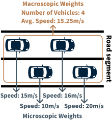
- (a) Macroscopic and microscopic weights.
- (b) Two layers of data sparsity.
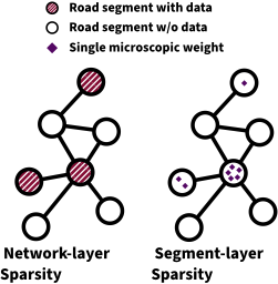
Figure 1: Motivation illustration.
that describe traffic conditions on the road network, which we term road network weights. Two types of such weights exist: macroscopic weights and microscopic weights, as exemplified in Figure 1a. Macroscopic weights describe aggregated traffic conditions, including numbers of vehicles on a road segment or the average speed of vehicles. Microscopic weights capture the vehicle-level traffic conditions, including individual vehicle's speed when traveling along a road segment or its travel time when traversing a road segment.
Macroscopic weights capture general traffic conditions on a road network and support tasks such as traffic flow [Guo et al., 2019] and congestion [Akhtar and Moridpour, 2021] prediction. While existing studies [Tedjopurnomo et al., 2020; Jiang and Luo, 2022; Jin et al., 2023] consider macroscopic weights, we target microscopic weights that capture finegrained, vehicle-level traffic conditions and support tasks such as traffic microsimulation [Hollander and Liu, 2008], driving behavior analysis [Abou Elassad et al., 2020], and routing with reliability guarantees [Hu et al., 2019]. More specifically, we focus on the problem of time-varying microscopic weight completion. The input is a road network and sparse microscopic weights observed within the current and historical time slots, where many segments lack weights within a time slot and segments with weights may have only few of them. The goal is to recover the accurate representation of weights for every road segment within the current time slot. This problem presents two unique challenges.
Solutions must contend with two layers of data sparsity. First, we have network-layer sparsity, as shown in Figure 1b①. In any time slot, the available vehicle movement data can be limited and thus may cover only a fraction of the entire road network. In other words, some road segments will have no microscopic weights during a time slot. Contending with this sparsity will require combining multiple information sources, including long-range spatial neighbors and long-term temporal history that include weights, as well as inherent information of road segments such as their typical microscopic weight distribution, in order to recover weights for road segments without weights.
Second, we have segment-layer sparsity, as shown in Figure 1b②. A road segment with microscopic weights may still contain too few weights to enable estimation of an accurate representation of the microscopic weights of the segment. This calls for sparsity-awareness to decide whether to rely more on available weights in case of low sparsity or to rely more on other information sources in case of high sparsity. Existing methods [Hu et al., 2019; Mu˜niz-Cuza et al., 2022; Han et al., 2022; Yuan et al., 2024] either disregard segmentlayer sparsity or simply discard all available data in segments with high sparsity, which increases network-layer sparsity.
Solutions must represent microscopic weights judiciously.
As discussed above, microscopic weights capture vehiclelevel traffic conditions. However, representing them directly as the set of all individual weights is inefficient, since the number of observed vehicles varies considerably across time and segments, making it difficult to derive accurate and generalizable representations from sparse weights. Rather, we need a representation that can capture complex traffic conditions accurately, including distributions with heavy tails and multiple clusters, while remaining interpretable and efficient.
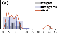
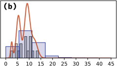
Most existing methods [Hu et al., 2019; Mu˜niz-Cuza et al., 2022; Han et al., 2022; Yuan et al., 2024] adopt histograms with fixed range and number of bins to represent microscopic weight distributions. However, such histograms face a trade-off between range coverage and resolution. For example, as shown in Figure 2, consider sets of microscopic weights with multiple clusters in the range [0, 15]. In case (a), a heavy tail value 41 forces the histogram to cover the range [0, 41], reducing resolution where most weights lie. In both cases, the fixed range and number of bins makes it difficult for histograms to distinguish the multiple clusters accurately, while Gaussian mixture models can capture these patterns flexibly. Diffusion models [Ho et al., 2020a; Wen et al., 2023a] are alternatives that can flexibly model complex distributions. However, they do not provide closedform representations, making them impractical for microscopic weight completion tasks that require explicit distribution information.
We propose Di-Sparsity Graph Gaussian Mixture Model (DiSGMM) for accurate time-varying microscopic weight completion. Design choices in DiSGMM address the above two challenges. First, to contend with the two layers of data sparsity, DiSGMM introduces two modules for learning latent embeddings of different information sources: one module for learning a static embedding for each road segment that incorporates inherent information; one module for learning a dynamic embedding for each road segment at a certain time slot, balancing known weights and inherent information with awareness of the segment-layer sparsity. DiSGMM also incorporates a spatiotemporal U-net with global residual connections, which is effective at gathering information from long-range spatial neighbors and long-term temporal history, thus contending with network-layer sparsity. Second, for the representation of microscopic weights, DiSGMM adopts a learnable Gaussian mixture model [Reynolds and others, 2009], which provides closed-form distributions while being flexible enough to capture complex traffic conditions including ones with heavy tails and multiple clusters. We report on extensive experiments on two real-world datasets that compare the performance of DiSGMM against several state-ofthe-art methods. Results providing evidence that DiSGMM achieves its design goal.
The paper's main contributions are summarized as follows:
- We propose DiSGMM, a novel method for time-varying microscopic weight completion on road networks that addresses two unique challenges of the problem.
- The method features a dual sparsity-aware architecture that combines static and dynamic embeddings with a spatiotemporal U-net, effectively handling both segment-layer and network-layer sparsity.
- The method enables learnable Gaussian mixture models for representing microscopic weights, providing closed-form distributions that flexibly represent complex traffic conditions with heavy tails and multiple clusters.
- We report on extensive experiments on two real-world datasets, finding that DiSGMM is able to consistently outperform state-of-the-art methods.
2 RelatedWork
Road network weight completion is a fundamental problem in traffic data mining, aiming to recover missing or incomplete weight information across road segments due to limitations in data collection. As mentioned in the introduction, we categorize road network weights into macroscopic and microscopic weights. Below, we briefly discuss macroscopic weight completion to provide context. Then we discuss existing microscopic weight completion studies, which represent alternatives to our proposal.
2.1 MacroscopicWeight Completion
Macroscopic weight completion has been studied extensively due to its importance in traffic monitoring and prediction. Existing methods can be categorized by their spatialtemporal modeling techniques. Tensor completion methods [Chen et al., 2022; Song et al., 2019] leverage lowrank assumptions to capture global patterns in traffic data, such as daily and weekly periodicity. RNN-based models [Hochreiter and Schmidhuber, 1997; Cao et al., 2018; Liu et al., 2019] capture temporal dependencies among consecutive time steps through sequential processing. GNNbased approaches [Kipf and Welling, 2017; Cini et al., 2022; Wu et al., 2021; Wei et al., 2024] explicitly model spatial correlations among road segments using road network structures. Attention-based methods [Shukla and Marlin, 2021; Nie et al., 2024; Vaswani et al., 2017] provide flexible long-range dependency modeling across both space and time. GANbased models [Goodfellow et al., 2014; Yoon et al., 2018; Li et al., 2019] and diffusion models [Tashiro et al., 2021; Liu et al., 2023] offer probabilistic imputation with uncertainty quantification.
However, macroscopic and microscopic weight completion have fundamentally different objectives and data characteristics. Macroscopic weights are aggregated measurements (e.g., average travel times, vehicle counts), and their completion focuses on recovering these aggregate statistics using available observations and spatiotemporal correlations. In contrast, microscopic weights capture vehicle-level traffic conditions, and their completion requires recovering the full distribution of weights for each road segment and time slot, not just aggregated statistics. Furthermore, microscopic weight completion faces unique challenges including the two layers of data sparsity and the need for appropriate representations of distributions, which are not concerns in macroscopic weight completion.
2.2 MicroscopicWeight Completion
Compared to macroscopic weight completion, microscopic weight completion has received much less attention. GCWC [Hu et al., 2019] is the first study to explicitly address microscopic weight completion. Instead of completing weights as single average values, GCWC completes weights as distributions in the form of histograms and uses a GCNbased network to complete the weight distributions of all road segments during a target time slot. While it considers spatial correlations between road segments, it disregards temporal correlations across different time slots. SSTGCN [Mu˜nizCuza et al., 2022] addresses this limitation by employing TCNs [Lea et al., 2016] and GCNs to capture both spatial and temporal correlations between road segments. It also introduces a mechanism to avoid propagating noisy information when dealing with high sparsity. ConGC [Han et al., 2022] further improves completion accuracy on sparse data by utilizing a graph containing contextual information of road segments, such as speed limits and numbers of lanes, to achieve higher accuracy when only few weights are known. However, the contextual information needed to build such graphs is not always available. Nuhuo [Yuan et al., 2024] partitions the road network into regions and uses a two-level encoding scheme: a global encoder captures inter-region correlations, while a local encoder models fine-grained spatial and temporal patterns within each region.
However, existing methods do not tackle the two challenges identified in the introduction. First, while they address network-layer sparsity through spatial and temporal modeling, they do not explicitly handle segment-layer sparsity, failing to adaptively adjust their reliance on sparse weights versus other information sources. Second, all existing methods use histograms to represent microscopic weights, which face a trade-off between range coverage and resolution that makes it difficult to represent complex distributions such as ones including heavy tails and multiple clusters.
3 Preliminaries
Definition 1 (Road Network). A road network is modeled as a directed graph G = (V, E), where V is a set of nodes vi that represent road intersections or endpoints of road segments and where E is a set of directed edges ei = (vj, vk) that represent road segments. Each edge e has an associated length le that captures the length of the segment it represents.
Definition 2 (Vehicle-level Travel Speed). For a road segment e with length le, the vehicle-level travel speed is defined as s = le/∆t, where ∆t is the time elapsed between a vehicle entering and leaving the segment.
Definition 3 (Time-varyingMicroscopicWeights). In a road network G, during a time slot T = [t1 , t2 ), each road segment e ∈ E is associated with a set of microscopic weights WTe , where each element is the vehicle-level travel speed of a vehicle that traverses segment e during time slot T. We adopt travel speed rather than travel time as the weight because speed is normalized by segment length, enabling direct comparison across segments. In contrast, travel times scale with segment length.
Problem definition. Time-varying microscopic weight completion. Given a road network G = (V, E) and a sequence of historical time slots ⟨T1, T2, . . . , TH-1⟩ along with the current time slot TH, where Ti = [t1i , t2i ), we have microscopic weights {WT1 e ,WT2 e , . . . ,WTH e } for each road segment e ∈ E. Note that some sets WTi e may be empty or sparse due to limited data coverage. The goal is to estimate an accurate representation of the microscopic weight distribution for element inWTH e across all road segments in E.
4 Methodology
As shown in Figure 3, DiSGMM addresses the two unique challenges of microscopic weight completion as follows. For the first challenge of two layers of sparsity, DiSGMM incorporates three main modules: a static road segment embedding module that captures inherent information of each road segment from network topology and historical weights; a sparsity-aware dynamic embedding module that balances known weights and inherent information with awareness of segment-layer sparsity; and a spatiotemporal U-net with global residual connections that gathers information from long-range spatial neighbors and long-term temporal history, contending with network-layer sparsity. For the second challenge of representation of microscopic weights, DiSGMM adopts learnable Gaussian mixture models, providing closedform distributions of microscopic weights that flexibly capture complex traffic conditions including heavy tails and multiple clusters.
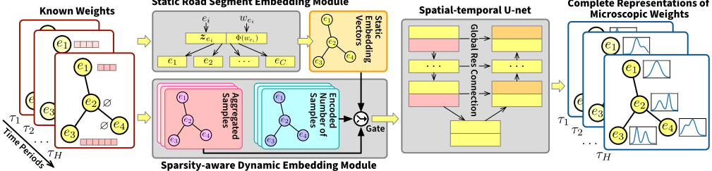
The following sections detail each module of DiSGMM.
4.1 Static Road Segment Embedding
The microscopic weight distribution of a road segment is closely tied to its inherent properties. To capture such properties without relying on additional contextual information, we design a static embedding module that learns the static embedding vector of each road segment from two sources: (1) network topology, reflecting a segment's role and neighboring structure, and (2) historical weight patterns, since segments with similar historical microscopic weights typically share similar properties.
For topology, we perform random walks on the road network G following DeepWalk [Perozzi et al., 2014] to generate sequences of contextual segments around each target segment e. For historical patterns, we collect the microscopic weights of e across all historical time slots.
We then employ an objective inspired by skipgram [Mikolov et al., 2013] that maximizes the cooccurrence probability of contextual segments given the target segment and its historical weights. Specifically, we assign a static embedding vector ze ∈ Rd to each segment e, an output vector z′ek ∈ R2d to each contextual segment, and encode each historical weight we using learnable Fourier features Φ(we) ∈ Rd [Li et al., 2021]. The objective is:
where || denotes concatenation and {e1, . . . , eC} are contextual segments from the random walk. This ensures that segments with similar topology and historical weight distributions learn similar embeddings ze, encoding their inherent, time-invariant properties. The detailed formulation is provided in Appendix.
4.2 Sparsity-aware Dynamic Embedding
During a specific time slot Tj, most road segments have few known microscopic weights, presenting segment-layer sparsity. The sparsity-aware dynamic embedding module addresses this by adaptively balancing two information sources: (1) the aggregated known weights of the segment during the time slot, and (2) the static embedding vector ze learned in Section 4.1, which captures inherent segment properties.
We first aggregate known weights WTj e using learnable Fourier features and a Transformer encoder [Vaswani et al., 2017], yielding AggTj e ∈ Rd . To incorporate sparsityawareness, we encode the number of known weights |WTj e | into a hidden vector ΨTj e using learnable Fourier features, then employ a gate mechanism [Chung et al., 2014] to balance the two sources:
where f Tj e is a forget gate controlled by the sparsity encoding, ˆhTj e is a candidate hidden vector combining both sources, and hTj e is the dynamic embedding vector of segment e during time slot Tj. When fewer weights are known (higher sparsity), the gate relies more on the static embedding ze; when more weights are available, it incorporates more from the aggregated known weights. The detailed formulation is provided in Appendix.
4.3 Spatiotemporal U-net with Global Residual Connections
Accurate microscopic weight completion relies heavily on long-range spatial correlations and long-term temporal dependencies. To effectively model such correlations and address network-layer sparsity, we propose a spatiotemporal Unet with global residual connections, building upon the U-net architecture [Ronneberger et al., 2015; Ho et al., 2020b].
The spatiotemporal U-net consists of spatiotemporal residual (STRes) blocks and down/up-sampling blocks organized in three components: the left component with Lres pairs of STRes and down-sampling blocks, the middle component with two STRes blocks, and the right component with Lres pairs of STRes and up-sampling blocks.
STRes and Down/Up-Sampling Blocks
Following UGnet [Wen et al., 2023b], each STRes block captures spatiotemporal correlations through temporal convolution (TCN [Lea et al., 2016]) followed by spatial convolution (GCN), with a residual connection. The input to the first STRes block is the collection of dynamic embeddings hTj e from all segments across all time slots, forming H ∈ R|E|×H×d . Subsequent blocks take outputs from previous blocks.
The down-sampling blocks halve the temporal dimension while doubling the feature dimension, enabling effective modeling of long-term temporal correlations. The upsampling blocks perform the reverse operation. This multiscale structure avoids excessive stacking of STRes blocks, which can cause vanishing gradients. Detailed formulations are provided in Appendix.
Global Residual Connections
In most U-net architectures, residual connections exist from the left component to the right component to facilitate effective training. We introduce global residual connections to enhance the modeling of long-range spatial correlations and further address network-layer sparsity.
We first partition the edge set E of road network G into nonintersecting clusters using the Louvain algorithm [Blondel et al., 2008]:
where Ej is a set of edges belonging to the j-th cluster and Ncls is the number of clusters.
For each STRes block in the left component, we perform cluster-level mean pooling on its input H to obtain a clustered hidden state for the j-th cluster:
We then expand the clustered representations back to segment-level by fetching each segment's cluster representation with positional encoding:
where ei belongs to the j-th cluster and PE is positional encoding [Vaswani et al., 2017] to distinguish different segments within a cluster. The expanded representations Hexp ∈ R|E|×Nin×din are concatenated with H along the feature dimension as residual input to the corresponding STRes block in the right component.
By establishing residual connections based on graph clustering, the spatiotemporal U-net extracts long-range spatial correlations without excessive stacking of GCN layers, which can cause over-smoothing.
4.4 Learnable GaussianMixture Model
To address the challenge of microscopic weight representation, we adopt learnable Gaussian mixture models (GMMs). Unlike histograms whose accuracy is severely affected by heavy tails, and diffusion models that lack closed-form representations, GMMs provide closed-form distributions that flexibly capture complex traffic conditons including heavy tails and multiple clusters.
From the output of the spatiotemporal U-net ¯H ∈ R|E|×H×d , we estimate the GMM for each segment e and time slot Tj by applying three prediction heads on ¯HTj e :
where Wϕ,Wµ,Wσ ∈ Rd×K and bϕ, bµ, bσ ∈ RK are learnable parameters, and K is the number of Gaussian components.
To train the model, we maximize the likelihood of p(wTj e ) for all observed microscopic weights. Given a ground truth weight w, the loss is:
While inference typically completes weights only for the most recent time slot TH, we train on all time slots in T to enhance model effectiveness.
5 Experiments
5.1 Datasets
We utilize two microscopic weight datasets referred to as HTT and CD. Both datasets are organized into records of vehicle-level travel speeds (m/s) on road segments.
The HTT dataset was published at the KDD Cup 2017 1 for a highway tollgate traffic flow prediction competition. It contains travel times of 24 road segments recorded by loop detectors located in a highway tollgate network. The data covers 19/07/2016 to 31/10/2016. We calculate travel speeds of road segments utilizing the travel times and road segment lengths in the datasets.
The CD dataset was released by Didi 2 and consists of GPS trajectories of taxis operating in Chengdu during 01/10/2018 to 01/12/2018. We fetch the road network of Chengdu from OpenStreetMap 3 and map-match [Yang and Gid´ofalvi, 2018] the trajectories onto the road network. The travel speeds of road segments are then calculated based on the map-matched trajectory points. To have a sufficient number of ground truth weights for evaluation, we select road segments in the central region of Chengdu and use the largest connected subgraph consisting of 194 road segments.
For both datasets, we divide a day into 96 15-minute time slots. This allows us to form a set of time-varying microscopic weights for each segment and time slot. The original missing rate of a dataset is defined the number of empty sets divided by the total number of sets in the dataset. Given the above settings, the original missing rates of HTT and CD are 31.918% and 33.766%, respectively.
2 https://gaia.didichuxing.com/
3 https://www.openstreetmap.org/
To ensure that the completed representation of weight distributions can be evaluated, we follow the practice of GCWC and use target missing rates to process the input weights to models. Specifically, for each time slot, given a target missing rate r, we remove all known weights of randomly selected road segments so that there are at least a fraction r of road segments miss known weights. The processed sets of weights are given as inputs to the models, and the unprocessed sets are used as the ground truth. In our experiments, four target missing rates are used: r = 50%, 60%, 70%, and 80%.
5.2 ComparisonMethods
The following methods are direct comparison with the proposed method on microscopic weight completion.
- Historical Average (HA): gathers all historical weights for the target road segment and estimates the density. We use two variants: HA-Hist and HA-GMM to estimate the distributions as histograms and Gaussian mixture models, respectively.
- GCWC [Hu et al., 2019]: utilizes GCN-based graph pooling to complete the stochastic weights of road segments.
- SSTGCN [Mu˜niz-Cuza et al., 2022]: combines TCNs and GCNs to model spatiotemporal correlations between road segments.
- ConGC [Han et al., 2022]: introduces a contextual graph for incorporating contextual features of road segments.
- Nuhuo [Yuan et al., 2024]: partitions the road network into regions and uses a two-level encoding scheme with global and local encoders. We also construct a variant NuhuoGMM by modifying the original output distributions from histograms to Gaussian mixture models.
We also include two state-of-the-art macroscopic weight completion methods with uncertainty consideration for comparison. Both methods share the technical similarity with microscoic weight completion: they estimate weight distributions. Do note that since they focus on macroscopic weight, the distribution estimation design is to take the uncertainty of statistics into consideration. This is fundamentally different from methods focus on microscopic weights.
- STGNF [An et al., 2024]: combines conditional normalizing flows with spatiotemporal graph learning to predict the probability distribution of macroscopic weights.
- PriSTI [Liu et al., 2023]: employs conditional diffusion probabilistic models with spatiotemporal attention to estimate the probability distribution of macroscopic weights.
5.3 Settings
For both datasets, we split the time periods by 8:1:1 to create the training, validation, and testing sets. Models are trained on the training set and evaluated on the testing set. The validation set is used for hyper-parameter tuning and for implementing early-stopping techniques.
To compare the accuracy of various types of distributions fairly, we employ two metrics: likelihood [Shao, 2003] and Continuous Ranked Probability Score (CRPS) [Matheson and Winkler, 1976]. Given an estimated weight distribution p and a ground truth weight w, the likelihood is directly calculated as the probability of p at observation w, and CRPS is calculated as CRPS(p, x) = ∫R(p(z) - I(x ≤ z))2dz, where I an indicator function which equals one if x ≤ z, and equals zero otherwise. These metrics assess how well the estimated distributions align with the recorded microscopic weights. A higher likelihood and a lower CRPS indicate better performance in the experiment. Note that likelihood cannot be calculated on methods that do not provide closed-form distributions, like PriSTI.
The proposed method is implemented using PyTorch [Paszke et al., 2019]. The five key hyper-parameters of the proposed method and their optimal values are H = 16, Lagg = 2, Lres = 2, d = 128, and K = 4. The effectiveness of these hyper-parameters are also discussed in Appendix. For the comparison methods, we set their hyper-parameters to the optimal values indicated in their respective papers, and use 8 bins for histograms. We utilize the contextual information in datasets, including lengths and levels of segments, to build the contextual graph for ConGC. Each experiment is repeated 5 times, and the mean and variance of the results are reported.
5.4 Performance Comparison
Table 1 presents the overall performance of the methods. The estimated weight distributions are also visualized in Appendix.
We have the following observations. First, among the histogram-based microscopic weight completion methods, Nuhuo achieves the best performance by leveraging a twolevel encoding scheme that captures both global and local spatial patterns. GCWC and SSTGCN, which model spatial or spatiotemporal correlations, outperform the simple historical average baseline HA-Hist. ConGC further improves accuracy by incorporating contextual features of road segments.
Second, methods that model microscopic weights as GMMs generally achieve higher accuracy than histogrambased methods. Histograms are limited by their predefined range and number of bins, making it difficult to accurately capture the underlying weight distributions. In contrast, GMMs can adapt to complex traffic conditions by learning appropriate means, variances, and mixture weights. This advantage is reflected in the performance gap between Nuhuo and Nuhuo-GMM, where the GMM variant consistently outperforms its histogram counterpart.
Third, the macroscopic weight completion methods, STGNF and PriSTI, show mixed results. STGNF is designed for traffic prediction rather than completion, and thus does not explicitly consider either layer of sparsity; its performance degrades notably at high missing rates. PriSTI models only macroscopic weights (aggregated statistics) and does not account for segment-level sparsity, which limits its effectiveness in the microscopic setting.
Fourth, DiSGMM achieves the best performance among all methods. While Nuhuo and Nuhuo-GMM address networklayer sparsity through their encoding schemes, they do not explicitly model segment-level sparsity. DiSGMM addresses
| Datasets | Methods | Likelihood (%) ↑ | CRPS ↓ | ||||||
|---|---|---|---|---|---|---|---|---|---|
| r = 50% | r = 60% | r = 70% | r = 80% | r = 50% | r = 60% | r = 70% | r = 80% | ||
| HA-Hist | 7.290±0.00 | 7.300±0.01 | 7.288±0.01 | 7.288±0.00 | 2.344±0.00 | 2.345±0.00 | 2.346±0.00 | 2.346±0.00 | |
| GCWC | 9.343±0.10 | 9.167±0.06 | 8.960±0.05 | 8.576±0.10 | 2.134±0.01 | 2.160±0.01 | 2.180±0.03 | 2.226±0.02 | |
| SSTGCN | 10.079±0.16 | 9.762±0.15 | 9.362±0.12 | 8.623±0.13 | 2.111±0.02 | 2.146±0.03 | 2.189±0.02 | 2.229±0.03 | |
| ConGC | 10.243±0.20 | 9.981±0.23 | 9.717±0.25 | 9.233±0.25 | 2.098±0.03 | 2.119±0.04 | 2.137±0.04 | 2.183±0.03 | |
| HTT Nuhuo | 11.203±0.20 | 10.564±0.23 | 10.059±0.13 | 9.481±0.12 | 2.078±0.01 | 2.104±0.02 | 2.128±0.01 | 2.173±0.01 | |
| HA-GMM | 6.989±0.03 | 6.959±0.03 | 6.974±0.02 | 6.991±0.04 | 2.364±0.00 | 2.367±0.00 | 2.365±0.00 | 2.365±0.00 | |
| STGNF | 12.195±0.15 | 11.268±0.17 | 10.445±0.10 | 9.083±0.19 | 2.087±0.02 | 2.112±0.01 | 2.183±0.02 | 2.283±0.02 | |
| PriSTI | - | - | - | - | 2.055±0.04 | 2.082±0.04 | 2.115±0.03 | 2.169±0.03 | |
| Nuhuo-GMM | 12.915±0.15 | 12.446±0.13 | 11.724±0.13 | 10.779±0.10 | 2.032±0.01 | 2.062±0.02 | 2.101±0.02 | 2.165±0.02 | |
| DiSGMM (ours) | 14.745±0.12 | 13.964±0.22 | 12.948±0.23 | 11.619±0.23 | 1.936±0.01 | 1.972±0.01 | 2.004±0.02 | 2.067±0.01 | |
| HA-Hist | 6.444±0.00 | 6.438±0.00 | 6.436±0.01 | 6.442±0.02 | 2.628±0.00 | 2.630±0.00 | 2.628±0.00 | 2.630±0.00 | |
| GCWC | 7.704±0.04 | 7.633±0.05 | 7.508±0.12 | 7.440±0.07 | 2.365±0.02 | 2.378±0.01 | 2.381±0.02 | 2.388±0.02 | |
| SSTGCN | 8.663±0.07 | 8.321±0.05 | 7.828±0.10 | 7.224±0.07 | 2.226±0.02 | 2.321±0.03 | 2.447±0.04 | 2.640±0.03 | |
| ConGC | 8.466±0.17 | 8.353±0.14 | 8.357±0.27 | 8.158±0.16 | 2.293±0.02 | 2.333±0.04 | 2.311±0.04 | 2.351±0.04 | |
| CD Nuhuo | 9.559±0.25 | 9.107±0.19 | 8.705±0.23 | 8.444±0.13 | 2.246±0.01 | 2.287±0.02 | 2.304±0.04 | 2.343±0.02 | |
| HA-GMM | 7.469±0.02 | 7.421±0.01 | 7.463±0.02 | 7.485±0.00 | 2.519±0.01 | 2.525±0.00 | 2.518±0.01 | 2.517±0.00 | |
| STGNF | 13.957±0.18 | 11.925±0.53 | 10.217±0.36 | 8.555±0.15 | 2.109±0.04 | 2.195±0.06 | 2.371±0.06 | 2.582±0.06 | |
| PriSTI | - | - | - | - | 2.135±0.05 | 2.185±0.05 | 2.268±0.06 | 2.315±0.06 | |
| Nuhuo-GMM | 13.905±0.22 | 12.878±0.23 | 11.690±0.24 | 10.368±0.15 | 2.116±0.02 | 2.165±0.03 | 2.232±0.03 | 2.273±0.03 | |
| DiSGMM (ours) | 16.388±0.13 | 15.027±0.14 | 13.403±0.22 | 11.835±0.15 | 1.996±0.03 | 2.043±0.02 | 2.114±0.05 | 2.145±0.03 | |
Bold denotes the best result, and underline denotes the second-best result.
| Methods | Likelihood (%) ↑ | CRPS ↓ | ||||||
|---|---|---|---|---|---|---|---|---|
| r = 50% | r = 60% | r = 70% | r = 80% | r = 50% | r = 60% | r = 70% | r = 80% | |
| -Sparsity | 14.696±0.30 | 13.591±0.28 | 12.603±0.22 | 11.198±0.14 | 1.940±0.02 | 1.984±0.01 | 2.010±0.01 | 2.071±0.03 |
| -Static | 13.420±0.15 | 13.040±0.21 | 12.018±0.37 | 10.813±0.31 | 1.962±0.01 | 2.003±0.02 | 2.058±0.03 | 2.098±0.04 |
| -DS | 13.026±0.07 | 12.716±0.05 | 11.436±0.22 | 10.283±0.18 | 1.991±0.02 | 2.015±0.02 | 2.087±0.02 | 2.171±0.02 |
| -Global Res | 14.565±0.20 | 13.643±0.18 | 12.410±0.23 | 11.462±0.15 | 1.946±0.02 | 1.981±0.01 | 2.018±0.03 | 2.074±0.03 |
| DiSGMM (full) | 14.745±0.12 | 13.964±0.22 | 12.948±0.23 | 11.619±0.23 | 1.936±0.01 | 1.972±0.01 | 2.004±0.02 | 2.067±0.01 |
Bold denotes the best result, and underline denotes the second-best result.
Table 2: Performance of DiSGMM's variants and the full model.
both layers of sparsity: it calculates sparsity-aware embeddings that effectively capture sparsity at the segment level, and employs a spatiotemporal U-net architecture to capture long-range correlations across the network. This comprehensive treatment of sparsity enables DiSGMM to achieve superior accuracy in microscopic weight completion.
5.5 Ablation Study
To assess the effectiveness of the components of DiSGMM, we compare the performance of the complete method against four variants:
- -Sparsity: removes sparsity-awareness from the gated mechanism in Equation 2. Specifically, makes f Tj e = σ(W ′f AggTj e +U ′f ze +bf).
- -Static: removes the static road segment embedding module and uses instead the vanilla node2vec for learning road segment embeddings.
- -DS: removes both sparsity-awareness and static embeddings, and uses Agg(WTj e ) from as the hidden state hTj e .
- -Global Res: removes the global residual connections.
The performance of these variants on the HTT dataset is reported in Table 2. First, comparing the variants -Sparsity,
-Static, and -DS with the full model, we find that the sparsityawareness of the gated mechanism in Equation 2 and the static road segment embedding module both improve the performance of DiSGMM. Removing either or both of these designs leads to a drop in the completion accuracy. Second, comparing the variant -Global Res with the full model, we observe that the global residual connections in the proposed spatiotemporal U-net are effective. Removing these connections impacts the model's ability to capture long-range spatial correlations negatively and results in worse performance.
6 Conclusion
We propose DiSGMM, a novel method for time-varying microscopic weight completion on road networks that addresses two unique challenges. For the two layers of sparsity, DiSGMM incorporates sparsity-aware embeddings that effectively leverage sparse observations alongside learned segment properties, and a spatiotemporal U-net with global residual connections that captures long-range correlations. For representation design, DiSGMM adopts learnable Gaussian mixture models, providing closed-form distributions that flexibly capture complex traffic conditions. Extensive experiments on two real-world datasets demonstrate that DiSGMM consistently outperforms state-of-the-art methods.
Ethical Statement
There are no ethical issues.
Use of large language models (LLMs). The use of LLMs in this work is restricted to two aspects: 1) For proofreading purposes after the drafting of this paper is complete; 2) For writing code to convert numerical experimental results into illustration plots.
Acknowledgments
This work was partially supported by National Natural Science Foundation of China (62472174). Supported by ECNU Multifunctional Platform for Innovation (001).
@inproceedings{ijcai2026p315,
  title     = {DiSGMM: A Method for Time-varying Microscopic Weight Completion on Road Networks},
  author    = {Lin, Yan and Hu, Jilin and Guo, Shengnan and Jensen, Christian S. and Lin, Youfang and Wan, Huaiyu},
  booktitle = {Proceedings of the Thirty-Fifth International Joint Conference on
               Artificial Intelligence, {IJCAI-26}},
  publisher = {International Joint Conferences on Artificial Intelligence Organization},
  editor    = {Diego Calvanese},
  pages     = {2834--2842},
  year      = {2026},
  month     = {8},
  note      = {Main Track},
  doi       = {10.24963/ijcai.2026/315},
  url       = {https://doi.org/10.24963/ijcai.2026/315},
}
TY - CPAPER TI - DiSGMM: A Method for Time-varying Microscopic Weight Completion on Road Networks AU - Lin, Yan AU - Hu, Jilin AU - Guo, Shengnan AU - Jensen, Christian S. AU - Lin, Youfang AU - Wan, Huaiyu T2 - Proceedings of the Thirty-Fifth International Joint Conference on Artificial Intelligence, IJCAI-26 PB - International Joint Conferences on Artificial Intelligence Organization PY - 2026 SP - 2834 EP - 2842 DO - 10.24963/ijcai.2026/315 UR - https://doi.org/10.24963/ijcai.2026/315 ER -Copied
Machine-readable versions of this paper, for tools and AI agents:





