
Graph Label Denoising via Neighborhood Agreement–Guided Expectation Maximization
Proceedings of the Thirty-Fifth International Joint Conference on Artificial Intelligence. Main Track. Pages 2852-2860.
https://doi.org/10.24963/ijcai.2026/317
Keywords
- Machine Learning: Weakly supervised learning
- Data Mining: Mining graphs
Abstract
Graph Neural Networks are susceptible to label noise, in which message-passing mechanisms serve as conduits for propagating erroneous supervision. Current mitigation techniques typically recover clean labels via heuristics that lack theoretical grounding, which often leads to ineffective denoising. To tackle the issue, we propose NAEM, a latent label estimation framework that models clean labels as latent variables by integrating neighborhood agreement into the Expectation-Maximization (EM) paradigm. To overcome the posterior collapse problem in standard EM under severe noise, we design a structure-aware E-step that leverages neighborhood agreement as a structural prior. This mechanism acts as a dynamic confidence gate based on local consensus to prevent the model from overfitting to noise. Simultaneously, by explicitly modeling the noise transition matrix in the M-step, NAEM decouples noise dynamics from semantic representation learning. Extensive experiments on five benchmark datasets demonstrate that NAEM consistently outperforms SOTA methods under varying noise conditions, validating the effectiveness of our framework.
- [Chen et al., 2024] Ling-Hao Chen, Yuanshuo Zhang, Tao- hua Huang, Liangcai Su, Zeyi Lin, Xi Xiao, Xiaobo Xia, and Tongliang Liu. Erase: Error-resilient representation learning on graphs for label noise tolerance. In Proceed- ings of the 33rd ACM International Conference on In- formation and Knowledge Management, CIKM '24, page 270-280, New York, NY, USA, 2024. Association for Computing Machinery.
- [Cheng et al., 2024] Yao Cheng, Caihua Shan, Yifei Shen, Xiang Li, Siqiang Luo, and Dongsheng Li. Resurrect- ing label propagation for graphs with heterophily and label noise. In Proceedings of the 30th ACM SIGKDD confer- ence on knowledge discovery and data mining, pages 433- 444, 2024.
- [Dai et al., 2021] Enyan Dai, Charu Aggarwal, and Suhang Wang. Nrgnn: Learning a label noise resistant graph neu- ral network on sparsely and noisily labeled graphs. In Pro- ceedings of the 27th ACM SIGKDD Conference on Knowl- edge Discovery & Data Mining, KDD '21, page 227-236, New York, NY, USA, 2021. Association for Computing Machinery.
- [Dempster et al., 1977] Arthur P Dempster, Nan M Laird, and Donald B Rubin. Maximum likelihood from incom- plete data via the em algorithm. Journal of the royal statis- tical society: series B (methodological), 39(1):1-22, 1977.
- [Du et al., 2021] Xuefeng Du, Tian Bian, Yu Rong, Bo Han, Tongliang Liu, Tingyang Xu, Wenbing Huang, Yixuan Li, and Junzhou Huang. Noise-robust graph learning by estimating and leveraging pairwise interactions. arXiv preprint arXiv:2106.07451, 2021.
- [Goldberger and Ben-Reuven, 2017] Jacob Goldberger and Ehud Ben-Reuven. Training deep neural-networks using a noise adaptation layer. In International conference on learning representations, 2017.
- [Han et al., 2018] Bo Han, Quanming Yao, Xingrui Yu, Gang Niu, Miao Xu, Weihua Hu, Ivor Tsang, and Masashi Sugiyama. Co-teaching: Robust training of deep neural networks with extremely noisy labels. Advances in neural information processing systems, 31, 2018.
- [Hu et al., 2020] Weihua Hu, Matthias Fey, Marinka Zitnik, Yuxiao Dong, Hongyu Ren, Bowen Liu, Michele Catasta, and Jure Leskovec. Open graph benchmark: datasets for machine learning on graphs. In Proceedings of the 34th International Conference on Neural Information Process- ing Systems, NIPS '20, Red Hook, NY, USA, 2020.
- Curran Associates Inc. [Kipf and Welling, 2016]
- Thomas N Kipf and Max Welling. Semi-supervised classification with graph convolutional networks. arXiv preprint arXiv:1609.02907, 2016.
- [Li et al., 2021] Yayong Li, Jie Yin, and Ling Chen. Uni- fied robust training for graph neural networks against label noise. In Pacific-Asia conference on knowledge discovery and data mining, pages 528-540. Springer, 2021.
- [Li et al., 2024] Xianxian Li, Qiyu Li, Haodong Qian, Jinyan Wang, et al. Contrastive learning of graphs under label noise. Neural networks, 172:106113, 2024.
- [Li et al., 2025] Kailai Li, Jiawei Sun, Jiong Lou, Zhanbo Feng, Hefeng Zhou, Chentao Wu, Guangtao Xue, Wei Zhao, and Jie Li. Leveraging peer-informed label con- sistency for robust graph neural networks with noisy la- bels. In Proceedings of the Thirty-Fourth International Joint Conference on Artificial Intelligence, pages 5598- 5606, 2025. IJCAI
- [NT et al., 2019a] Hoang NT, Choong Jun Jin, and Tsuyoshi Murata. Learning graph neural networks with noisy labels. arXiv preprint arXiv:1905.01591, 2019.
- [NT et al., 2019b] Hoang NT, Choong Jun Jin, and Tsuyoshi Murata. Learning graph neural networks with noisy labels. arXiv preprint arXiv:1905.01591, 2019.
- [Qian et al., 2023] Siyi Qian, Haochao Ying, Renjun Hu, Jingbo Zhou, Jintai Chen, Danny Z. Chen, and Jian Wu. Robust training of graph neural networks via noise gover- nance. In Proceedings of the Sixteenth ACM International Conference on Web Search and Data Mining, WSDM '23, page 607-615, New York, NY, USA, 2023. Association for Computing Machinery.
- [Sen et al., 2008] Prithviraj Sen, Galileo Namata, Mustafa Bilgic, Lise Getoor, Brian Galligher, and Tina Eliassi-Rad. Collective classification in network data. AI magazine, 29(3):93-93, 2008.
- [Shchur et al., 2018] Oleksandr Shchur, Maximil- ian Mumme, Aleksandar Bojchevski, and Stephan Günnemann. Pitfalls of graph neural network evaluation. arXiv preprint arXiv:1811.05868, 2018.
- [Velikovi et al., 2018] Petar Velikovi, Arantxa Casanova, Pietro Lio, Guillem Cucurull, Adriana Romero, and Yoshua Bengio. Graph attention networks. 6th Inter- national Conference on Learning Representations, ICLR 2018 -Conference Track Proceedings, 2018.
- [Wang et al., 2019] Yisen Wang, Xingjun Ma, Zaiyi Chen, Yuan Luo, Jinfeng Yi, and James Bailey. Symmetric cross entropy for robust learning with noisy labels. In Proceed- ings of the IEEE/CVF international conference on com- puter vision, pages 322-330, 2019.
- [Wang et al., 2024] Zhonghao Wang, Danyu Sun, Sheng Zhou, Haobo Wang, Jiapei Fan, Longtao Huang, and Ji- ajun Bu. Noisygl: A comprehensive benchmark for graph neural networks under label noise. Advances in Neural Information Processing Systems, 37:38142-38170, 2024.
- [Wei et al., 2020] Hongxin Wei, Lei Feng, Xiangyu Chen, and Bo An. Combating noisy labels by agreement: A joint training method with co-regularization. In Proceedings of the IEEE/CVF conference on computer vision and pattern recognition, pages 13726-13735, 2020.
- [Wei et al., 2023] Xiaowen Wei, Xiuwen Gong, Yibing Zhan, Bo Du, Yong Luo, and Wenbin Hu. Clnode: Cur- riculum learning for node classification. In Proceedings of the sixteenth ACM international conference on web search and data mining, pages 670-678, 2023.
- [Wu et al., 2024] Yuhao Wu, Jiangchao Yao, Xiaobo Xia, Jun Yu, Ruxin Wang, Bo Han, and Tongliang Liu. Mit- igating label noise on graphs via topological sample selec- tion. In Proceedings of the 41st International Conference on Machine Learning, ICML'24. JMLR.org, 2024.
- [Yuan et al., 2023] Jingyang Yuan, Xiao Luo, Yifang Qin, Yusheng Zhao, Wei Ju, and Ming Zhang. Learning on graphs under label noise. In ICASSP 2023-2023 IEEE In- ternational Conference on Acoustics, Speech and Signal Processing (ICASSP), pages 1-5. IEEE, 2023.
- [Zhang et al., 2020] Mengmei Zhang, Linmei Hu, Chuan Shi, and Xiao Wang. Adversarial label-flipping attack and defense for graph neural networks. In 2020 IEEE Inter- national Conference on Data Mining (ICDM), pages 791- 800, 2020.
- [Zhu et al., 2024] Yonghua Zhu, Lei Feng, Zhenyun Deng, Yang Chen, Robert Amor, and Michael Witbrock. Ro- bust node classification on graph data with graph and label noise. In Proceedings of the AAAI conference on artificial intelligence, volume 38, pages 17220-17227, 2024.
References were extracted automatically from the PDF and may contain errors.
Full text extracted automatically from the PDF; figures, tables and equations may differ. The PDF is the version of record.
1 Introduction
Graph Neural Networks (GNNs) have emerged as the dominant paradigm for representation learning on graph-structured data, demonstrating exceptional performance in node classification [Kipf and Welling, 2016; Velikovi et al., 2018]. Despite their success, GNNs often struggle in real-world settings due to unavoidable label noise from unreliable annotations or malicious attacks. While label noise is a well-studied topic in computer vision, its impact on graphs is more severe and complex due to the non-i.i.d. nature of the data. This message-passing paradigm transforms GNNs into effective spreaders of label noise. Unlike i.i.d. (independent and identically distributed) data, where noise is localized, graph edges facilitate the propagation of erroneous signals. Thus, a single noisy node can significantly compromise the learned representations of its clean neighbors through topological aggregation [NT et al., 2019a; Dai et al., 2021]. This topological dependency causes a cascading effect, where a few noisy labels can pollute large areas of the graph, significantly reducing model generalization.
∗Corresponding author
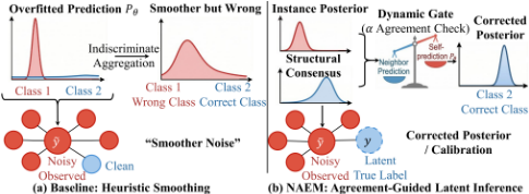
To mitigate this issue, recent research has adapted strategies from the i.i.d. domain, predominantly categorizing into sample selection and label correction. Sample selection methods, such as TSS [Wu et al., 2024] and CLNode [Wei et al., 2023], employ heuristics like the small-loss criterion to segregate clean nodes from noisy ones. While effective in low-noise regimes, these methods suffer from data starvation and confirmation bias as noise rates increase, leading the model to overfit early while discarding informative hard samples. Conversely, label correction approaches, such as NRGNN [Dai et al., 2021] and RTGNN [Qian et al., 2023], attempt to rectify noisy labels via neighborhood smoothing. However, these methods often apply graph smoothing indiscriminately based on the naive homophily assumption. As illustrated in Figure 1(a), we contend that employing noisedominated neighborhoods to refine node labels does not eliminate the noise within the graph; rather, it merely produces smoother noise.
A critical oversight in current methods is the formulation of the Clean Labelas a deterministic target to be recovered via a selection or smoothing paradigm. However, since ground truth is intrinsically unobservable under noisy conditions, we propose that it should be rigorously modeled as a Latent Variable within a probabilistic generative paradigm. We redefine the graph noisy learning task as maximum likelihood estimation via the EM algorithm [Dempster et al., 1977]. However, a major limitation of standard EM in noisy environments is its susceptibility to posterior collapse, which is particularly pronounced in graph learning since the topologydependent noise propagation pattern. As GNNs recursively encode noisy signals from neighbors into node representations, the model learns to interpret this noise as a valid structural pattern, resulting in self-reinforcing bias. The posterior converges towards the noisy observations ˜ Y with misleadingly high confidence. To alleviate posterior collapse on graph data, we integrate Neighborhood Agreement (NA) into the EM framework. NA acts as an informative structural prior to guide and refine the posterior estimation rather than serving as a hard constraint.
We propose NAEM, a structure-aware Neighborhood Agreement EM framework that provides a principled solution for denoising graph labels, as shown in Figure 1(b). Unlike heuristic approaches, NAEM maximizes the Expected Complete-Data Log-Likelihood of the observed noisy graph data. First, we design a structure-aware E-step that produces a refined posterior explicitly incorporating the neighborhood agreement mechanism. In detail, we leverage an adaptive agreement gate to refine inference based on structural consistency. It retains instance-level predictions for nodes aligned with their local neighbors, while adjusting inconsistent nodes towards the direction of neighborhood consensus, thereby mitigating overfitting to noisy labels. Moreover, during the corresponding adaptive M-step, we simultaneously optimize the GNN parameters and the noise transition matrix through iterative refinement. NAEM effectively disentangles corruption patterns from semantic features by explicitly modeling the noise transition process, facilitating robust representation learning across varied noise environments. Extensive experiments on five benchmark datasets show our method consistently outperforms baselines and enjoys great scalability under various noise conditions. Supplementary material is available at Zenodo 1 .
Our main contributions are in the following three-fold:
- We propose a probabilistic generative framework, named NAEM, that reformulates graph label noise learning as a latent variable estimation problem. We derive a unified optimization target with theoretical convergence guarantees.
- We design a structure-aware E-step that integrates Neighborhood Agreement as a structural prior. Through an adaptive gating mechanism, we dynamically refine the posterior to curb noisy signal propagation.
- Extensive experiments on five benchmark datasets demonstrate that NAEM consistently outperforms baselines under various noise conditions, and comprehensive analysis confirms the effectiveness and robustness of our framework.
1 https://doi.org/10.5281/zenodo.20098669
2 RelatedWork
2.1 Label Noise Learning on I.I.D. Data
Traditional independent and identically distributed label noise learning follows three paradigms: estimating the noise transition matrix, such as the S-model [Goldberger and BenReuven, 2017]; selecting clean samples based on the smallloss assumption, such as Co-teaching [Han et al., 2018] and JoCoR [Wei et al., 2020]; and employing robust objective functions, such as SCE [Wang et al., 2019]. However, these methods struggle with graph data where noise spreads through edges, as they overlook properties that depend on topology.
2.2 Label Noise Learning on Graphs
Graph noise learning in research is mainly categorized into sample selection, label correction, and representation learning.
Sample Selection Strategies
Similar to i.i.d. methods, these strategies train GNNs using only the estimated clean label set. CLNode [Wei et al., 2023] employs a curriculum learning strategy, while TSS [Wu et al., 2024] and RTGNN [Qian et al., 2023] utilize topology identification criteria and collaborative learning mechanisms, respectively. However, sample selection often leads to data insufficiency and degraded generalization performance when facing a severe noise setting.
Label Correction and Propagation
Conversely, these methods correct noise through smoothing or constraints. NRGNN [Dai et al., 2021], Union-NET [Li et al., 2021], and CGNN [Yuan et al., 2023] use naive neighborhood aggregation, while other methods incorporate structural guidelines such as community clustering [Zhang et al., 2020], pairwise interactions [Du et al., 2021], and backward loss correction [NT et al., 2019b]. However, random aggregation of noisy neighborhoods tends to produce smoother noise rather than clear signals, thereby enhancing confirmation bias.
Robust Representation and Contrastive Learning
Recent studies enhance GNN robustness by utilizing graph contrastive learning [Zhu et al., 2024; Li et al., 2024] or energy-based detection and prototype alignment [Chen et al., 2024; Li et al., 2025]. Although these methods enhance the robustness of features, they do not provide a unified probabilistic framework for inferring labels. Unlike existing works treating noisy labels as deterministic targets, our NAEM framework models the true label as a latent variable.
3 Methodology
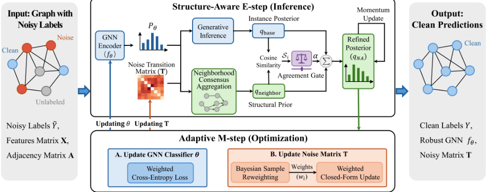
In this section, we present the proposed NAEM framework to mitigate graph label noise, as illustrated in Figure 2. Specifically, we formulate the noisy node classification problem as a likelihood maximization task involving a latent variable. Then, we incorporate a structure-aware prior during the inference stage to rectify the posterior estimation within the EM paradigm, followed by an adaptive maximization stage to decouple noise patterns from semantic representations.
3.1 ProblemFormulation
Let G = (V, E) denote an undirected graph where V = {v1, . . . , vN} is the set of N nodes and E is the set of edges. Let X ∈ RN×d be the node feature matrix and A ∈ {0, 1}N×N be the adjacency matrix. The node set V can be split into labeled set VL and unlabeled set VU, where usually |VL| ≪ |VU| in graph node classification task. The class set is C = {1, . . . ,K}.
The observed labeled set VL may be corrupted in the realworld settings. We represent the observed noisy labels as ˜ YL = {˜ yi | vi ∈ VL}, where ˜ yi ∈ C. We also assume that the latent clean labels, represented as Y = {yi | vi ∈ V}, are unobservable. The goal is to learn a robust GNN classifier fθ that can accurately predict the clean labels Y for both VL and VU under noisy supervision from ˜ YL.
3.2 Probabilistic Generative Framework
In contrast to sample selection paradigms, we model the label correction as a probabilistic inference problem. To estimate clean label, we establish a generative process connecting the latent clean Y and the noisy observation ˜ Y conditioned on graph data X and A.
Latent Label Generation. The clean label yi is generated based on node features X and graph structure A, and is implemented by the GNN parameters θ:
where fθ(·)k denotes the predicted probability for class k. Noisy Label Generation. Given the latent clean label yi, the observed noisy label ˜ yi is produced via a noise transition process. We adopt a class-dependent noise model defined by a transition matrix T ∈ [0, 1]K×K , following standard assumptions for graph label noise learning [Wang et al., 2024]:
where Tjk represents the probability that clean label j is corrupted into noisy label k. Our goal is to jointly infer the posterior distribution of the latent true labels Y and learn the robust classifier θ by maximizing the marginal likelihood:
As direct maximization is intractable, we employ the EM algorithm to maximize the Expected Complete-Data LogLikelihood (Q-function):
where Θ = {θ, T} and q(t) i (j) is the posterior estimate at iteration t. Detailed derivation in Supplementary Sec. A.1.
Standard EM estimates the posterior q(Y ) relying solely on the current model prediction Pθ and transition matrix T. Nevertheless, this phenomenon is especially harmful in graph learning because of the so-called topology-dependent noise propagation. Compared to i.i.d. data, where noise is typically associated with specific samples, the recursive messages that flow through GNNs may unintentionally carry misleading signal information from noisy neighbors into the node representations. This creates a self-reinforcing cycle where the model is led to believe that label noise is a valid structural pattern. As a result, the graph classifier fθ is more likely to overfit noisy labels with misleadingly high confidence, and the posterior collapses to the noisy observations, and hence it loses its ability to correct errors. To mitigate this, we introduce Neighborhood Agreement as a structural prior to calibrate the posterior inference in the E-step.
3.3 Structure-Aware E-Step
In the E-step, our objective is to estimate the posterior distribution of the clean labels q(t) (yi = j) ≈ P(yi = j | ˜ yi, xi,A). To prevent the posterior from being dominated by noisy supervision, we inject the graph structure as an inductive bias.
Initialization and Evidence Decomposition
Before the iterative process, we initialize the model parameters θ(0) via a warm-up phase using the standard crossentropy loss on ˜ YL for a few epochs. The transition matrix T(0) employs a diagonally dominant random initialization.
At iteration t, we decompose the evidence for the latent label yi into the instance-level posterior and the neighborhood consensus.
First, the instance-level posterior qbase represents the standard Bayesian update for node i, conditioning on its observed noisy label ˜ yi. It integrates the predictive distribution from the GNN classifier (acting as the latent prior) and the noise transition probability (acting as the observation likelihood):
The posterior remains heavily anchored to the current parameters θ(t) , rendering it susceptible to the bias of noisy labels during early training.
Second, we introduce the neighborhood consensus qneighbor to rectify potential biases in qbase. The proposed mechanism diverges from feature aggregation by enforcing explicit posterior smoothing within the label space, grounded in the graph homophily assumption. Pooling instance-level posteriors from neighboring nodes establishes a structural prior:
where N(i) = {vj ∈ V | Aij = 1} denotes the set of immediate neighbors of node vi.
Neighborhood Consistency and Posterior Refinement
To evaluate the reliability of the instance-level posterior, we compute the Neighborhood Agreement (NA) score Si ∈ [0, 1] for node i via the normalized cosine similarity between the two evidence views:
where qbase,i and qneighbor,i denote the probability vectors of q(t) base (yi) and q(t) neighbor (yi), respectively. A high Si signifies that the GNN prediction aligns with the local topology, typical of reliable samples, whereas a low agreement suggests a conflict indicative of label noise. Dynamic regulation of the neighborhood consensus influence relies on the computation of an adaptive agreement gate αi. Mapping Si to a confidence weight wi precedes the derivation of αi:
Here, τhigh and τlow are agreement thresholds determining the trust interval, and λNA is agreement strength controlling the maximum strength of the structural prior. The gating mechanism αi dynamically adjusts the mixing ratio by retaining the instance-level posterior for high-agreement nodes (wi ≈ 1) or enforcing neighborhood consensus correction as the coefficient approaches λNA under low-agreement conditions (wi ≈ 0). We derive the refined posterior q(t) NA(yi) via convex combination:
Finally, we apply a momentum coefficient hyperparameter, denoted as γ, to update the model to ensure stability:
3.4 Adaptive M-Step for Joint Optimization
In the M-step, we maximize the Q-function with respect to GNN parameters θ and transition matrix T given q(t) , decoupling semantic learning from noise modeling, as θ and T appear in separate terms in Eq. (4).
Robust Representation Learning (Updating θ)
The optimization for θ corresponds to minimizing the expected risk with respect to the latent labels. This is equivalent to minimizing a posterior-weighted cross-entropy loss:
Supervision of the GNN relies on the corrected latent distribution through the substitution of noisy one-hot targets ˜ yi with refined soft labels q(t) .
Noise Transition Estimation (Updating T)
NAEM explicitly learns the class-dependent noise pattern T to decouple noise patterns from semantic features. Maximizing the Q-function with respect to T under the constraint ∑k Tjk = 1 yields a weighted closed-form solution. To mitigate random outliers, Bayesian Sample Reweighting assigns each sample a transition-model reliability score ri, which estimates the posterior probability that the sample is generated by the structured transition process rather than a uniform outlier component; its closed-form definition and derivation are provided in the supplementary material, Sec. A.2. This leads to the Weighted Closed-Form Solution for the update rule at iteration t + 1:
Here I(·) denotes the indicator function. The symbol ri is distinct from the neighborhood-agreement confidence wi in Eq. (8). The estimation mechanism aggregates the fractional counts of estimated true labels j flipping to observed labels k weighted by sample reliability to approximate the noise transition probability. Algorithm details and complexity analysis are provided in Supplementary Sec. A.3; NAEM preserves the O(|E|d +Nd2 ) complexity inherent to the backbone GNN.
| Dataset | Cora | Citeseer | Pubmed | A-Computers | A-Photos | ||||
|---|---|---|---|---|---|---|---|---|---|
| Noise type | 30% PN 30%UN | 30% PN | 30%UN | 30% PN | 30%UN | 30% PN | 30%UN | 30% PN | 30%UN |
| GCN GAT | 65.36±5.54 71.06±4.39 62.93±4.04 65.53±4.01 | 53.66±5.03 50.90±4.78 | 55.05±3.11 52.88±3.07 | 62.91±5.49 59.77±4.19 | 66.53±6.23 60.64±6.43 | 70.95±4.21 68.78±4.58 | 77.26±3.34 76.11±2.75 | 79.26±4.79 79.46±4.23 | 84.86±3.27 85.64±2.61 |
| S-model Coteaching JoCoR SCE | 65.59±5.28 71.05±4.88 56.87±4.40 61.22±5.88 64.52±5.80 71.16±6.53 66.97±4.29 71.15±5.04 | 53.41±5.26 48.34±3.48 56.30±5.14 54.61±4.53 | 54.68±3.26 46.75±4.80 57.14±3.22 57.00±2.87 | 63.16±5.46 60.45±7.23 55.88±7.20 63.78±4.86 | 66.52±6.88 64.38±7.27 59.44±5.23 67.38±6.86 | 73.81±5.91 67.89±9.09 66.82±4.70 72.85±2.19 | 79.42±3.17 76.25±5.65 70.01±11.03 77.01±2.82 | 80.06±5.25 74.56±7.56 68.48±8.62 81.57±4.96 | 85.32±4.17 82.78±5.75 75.22±8.24 85.85±4.42 |
| NRGNN RTGNN CP CLNode PIGNN DGNN RNCGLN UnionNET CGNN CR-GNN R2LP TSS ERASE ProCon | 69.73±4.82 74.86±2.82 63.44±5.93 66.33±3.72 66.12±5.63 71.76±5.85 64.55±5.04 68.24±3.95 65.04±5.83 70.43±4.19 58.49±4.41 56.15±6.40 68.48±6.37 73.29±5.17 66.29±5.23 72.83±4.74 63.27±5.71 69.57±3.47 65.37±5.48 72.03±4.48 58.42±1.45 57.08±1.62 60.77±4.90 62.61±4.97 73.38±4.47 77.40±2.43 74.66±3.80 | 59.28±6.21 48.39±5.15 54.15±5.44 53.19±3.19 55.97±4.79 46.76±6.57 54.16±4.56 58.15±6.09 51.38±4.19 52.45±5.07 32.51±9.06 51.88±5.25 53.63±4.48 76.61±4.55 55.16±8.02 | 61.87±3.44 51.38±4.11 56.72±3.42 55.48±2.92 60.71±2.98 48.99±2.57 58.56±7.25 58.87±3.25 52.31±3.22 55.87±3.38 37.80±11.22 53.52±3.02 58.78±4.29 59.68±5.53 | 57.22±5.93 59.04±6.65 62.67±4.62 62.25±5.23 66.75±3.88 58.36±4.87 62.88±5.80 62.77±4.97 56.01±14.88 62.91±5.47 50.73±10.75 62.95±5.12 63.35±4.78 67.10±3.56 | 62.37±6.79 68.30±4.31 68.11±4.27 64.56±6.50 69.02±3.34 63.29±7.74 68.42±5.31 65.93±6.56 57.73±16.75 66.42±6.35 48.80±17.57 64.14±5.92 67.52±5.05 71.77±3.90 | 67.00±2.65 61.40±10.02 70.49±4.59 73.96±4.61 72.22±5.80 48.11±7.24 63.62±3.93 37.33±2.18 40.55±21.80 39.18±31.03 47.97±11.85 66.69±7.98 64.68±5.64 70.47±4.58 | 70.47±3.45 69.04±4.96 77.74±3.13 80.31±2.41 79.04±2.28 50.53±4.26 62.22±3.97 37.34±2.94 46.07±22.63 48.29±31.43 45.13±13.25 73.08±3.73 69.39±3.53 73.48±4.11 | 71.92±6.84 70.33±8.11 77.45±5.26 79.12±4.90 79.43±4.63 51.09±13.97 64.79±9.92 30.89±7.39 45.70±25.46 37.53±35.25 55.14±10.81 77.00±5.80 81.62±6.66 82.02±3.38 | 78.30±3.31 82.08±6.02 83.52±3.00 85.46±2.70 84.90±4.59 54.28±8.37 72.80±6.60 32.29±4.47 47.26±25.51 35.24±32.66 45.18±13.77 83.04±2.66 87.00±1.80 81.81±6.42 |
| NAEM | 78.50±3.99 81.70±0.93 | 61.54±4.08 | 68.29±1.74 | 68.13±6.55 | 72.90±4.88 | 82.41±1.75 | 84.96±1.00 | 89.06±1.56 | 90.75±0.78 |
4 Experiment
We evaluate the effectiveness of the proposed NAEM framework by addressing the following research questions:
- RQ1: Does NAEM outperform state-of-the-art baselines on node classification tasks under various noise settings?
RQ2: Can NAEM mitigate noise propagation and maintain accuracy under incorrect supervision?
RQ3: How does each component contribute to the overall performance of the framework?
RQ4: Does the Neighborhood Agreement strategy effectively prevent posterior collapse and enhance latent label inference?
4.1 Experimental Setup
Datasets
We evaluate NAEM on five benchmarks: Cora, Citeseer, Pubmed [Sen et al., 2008], Amazon-Computers, and Amazon-Photos [Shchur et al., 2018], with OGBN-Arxiv [Hu et al., 2020] and Flickr used for scalability and heterophily evaluation. Dataset details are available in Supplementary Sec. B.1.
Noise Injection
We follow standard protocols [Wang et al., 2024; Li et al., 2025] to inject synthetic label noise into the training set: Uniform Noise (UN): Uniformly flips the true label to another class with probability η. Formally, for ∀j ̸= i, p(˜ y = j | Y = i) = η c-1 , where c represents the number of classes. Pair Noise (PN): Flips the true label to its corresponding pair class with probability η. We test noise rates η ∈ {10%, 20%, 30%, 40%, 50%} for both types.
Baselines
We compare NAEM against baselines from three categories: Standard GNNs: GCN [Kipf and Welling, 2016], GAT [Velikovi et al., 2018].
Label Noise Learning (I.I.D.): S-model [Goldberger and Ben-Reuven, 2017], Co-teaching [Han et al., 2018], JoCoR [Wei et al., 2020], SCE [Wang et al., 2019].
Graph Label Noise: NRGNN [Dai et al., 2021], RTGNN [Qian et al., 2023], CP [Zhang et al., 2020], DGNN [NT et al., 2019b], Union-NET [Li et al., 2021], PIGNN [Du et al., 2021], CLNode [Wei et al., 2023], RNCGLN [Zhu et al., 2024], CGNN [Yuan et al., 2023], CRGNN [Li et al., 2024], TSS [Wu et al., 2024], ERASE [Chen et al., 2024], R2LN [Cheng et al., 2024], ProCon [Li et al., 2025].
To ensure a fair and rigorous comparison, for baselines included in the NoisyGL benchmark [Wang et al., 2024], we report the results directly from the original paper. For recent methods not covered by NoisyGL, we reproduce their results using their official implementations, strictly adhering to the experimental settings of NoisyGL. Implementation specifics of our method, including hyperparameter grid search ranges and optimization setups, are detailed in Supplementary Sec. B.2.
4.2 Performance Comparison (RQ1)
Main Result
Table 1 reports the test accuracy (mean ± std over 10 runs). NAEM consistently outperforms all baselines on five datasets under 30% noise. For instance, on Amazon-Computers (30%
| Dataset | Cora | Amazon-Computers | ||||||
|---|---|---|---|---|---|---|---|---|
| Metric | ACLT AILT | AUCS AUU | AUIS | ACLT | AILT | AUCS | AUU | AUIS |
| NRGNN RTGNN CP CLNode PIGNN DGNN RNCGLN UnionNET CGNN CR-GNN R2LP TSS ERASE ProCon | 84.53±4.07 75.64±6.68 82.29±3.33 71.57±8.33 98.77±1.49 32.04±14.17 94.14±3.44 34.88±9.96 98.43±1.55 29.19±20.67 81.06±10.80 37.58±15.48 99.00±1.18 13.44±8.24 98.60±1.18 33.89±15.53 97.16±2.79 31.37±10.72 96.39±1.92 34.93±8.11 99.14±0.92 1.71±2.26 88.20±9.53 14.94±10.08 91.30±2.54 75.17±8.41 94.46±3.71 64.49±11.99 | 83.11±3.16 81.33±2.25 75.53±4.80 73.44±4.95 80.85±3.46 72.32±4.45 76.77±3.30 67.11±5.11 80.30±4.69 70.28±8.69 70.89±7.28 63.60±6.94 77.06±3.30 75.36±3.33 82.45±2.69 73.46±3.70 80.41±3.62 70.38±4.04 80.09±2.90 71.75±4.73 71.68±3.39 55.45±1.98 74.12±3.68 62.28±5.48 82.31±2.58 76.49±2.75 82.13±3.43 75.99±4.54 | 78.81±5.94 69.50±8.06 51.46±12.99 43.86±7.48 49.25±16.24 45.72±10.64 72.92±4.66 52.59±9.00 46.81±10.04 51.88±6.64 44.48±4.78 38.71±9.03 78.94±5.30 73.86±10.43 | 61.82±5.95 73.58±7.57 88.51±4.38 92.01±2.61 93.43±2.98 37.44±10.38 84.67±10.92 13.17±4.37 44.71±32.57 53.11±30.63 17.15±7.48 85.16±7.87 85.66±3.52 84.80±2.68 | 52.34±7.43 65.89±6.97 70.81±4.68 75.59±4.39 70.94±7.66 37.92±9.60 26.18±13.75 13.20±5.35 38.55±29.40 43.38±24.06 20.79±8.86 49.93±14.11 66.10±6.72 74.96±3.14 | 72.48±5.35 72.57±5.67 82.29±3.76 84.09±2.50 83.08±2.38 50.31±8.42 58.66±4.12 26.42±5.21 47.06±24.61 52.15±30.77 32.54±13.66 73.47±3.94 72.70±5.50 75.62±5.21 | 71.15±5.00 71.37±5.33 80.65±4.00 82.77±2.99 81.69±3.08 49.28±7.37 57.63±3.75 26.26±5.46 46.04±24.70 51.12±30.06 45.35±19.41 73.62±4.46 68.45±3.85 72.58±4.33 | 69.03±6.67 67.42±6.79 77.52±4.44 80.19±5.43 79.78±5.93 46.11±7.94 54.96±6.97 21.99±7.48 42.20±26.69 48.21±29.15 31.88±12.50 66.16±6.69 70.73±4.79 76.82±4.49 |
| NAEM | 92.58±2.17 77.13±6.93 | 85.49±2.45 81.04±0.96 | 81.59±4.68 | 90.25±1.67 | 84.40±2.66 | 84.45±1.84 | 85.17±1.19 | 83.98±3.42 |
uniform noise), NAEM surpasses the runner-up CLNode by 4.65% (84.96% vs. 80.31%). Furthermore, NAEM demonstrates superior robustness against pair noise; on Citeseer (30% pair noise), it achieves 61.54%, significantly exceeding GCN (53.66%) and RTGNN (48.39%). Additionally, lower standard deviations confirm the stability of our principled probabilistic framework in modeling latent labels. Additional scalability results on the large-scale OGBN-Arxiv benchmark are provided in Supplementary Sec. B.4. The comparison with baselines demonstrates good scalability of our method on large-scale datasets.
Robustness against Varying Noise Rates
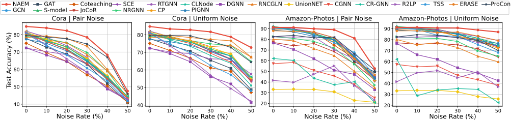
To evaluate model robustness, we varied noise rates from 0% to 50% as shown in Figure 3. NAEM consistently outperforms baselines in both settings. Under Uniform Noise, NAEM exhibits remarkable stability, widening the performance gap as noise intensity increases. In the more challenging Pair Noise scenarios, while all methods degrade due to structured label flipping, NAEM maintains a distinct lead over SOTA competitors. Competitive performance on clean data (0% noise) confirms that our method effectively handles noise without compromising the clean signal. To further test robustness beyond homophilic graphs, we report supplementary results on the heterophilic Flickr benchmark in Supplementary Sec. B.3. Comprehensive results on five datasets are detailed in Supplementary Sec. B.8.
4.3 Analysis of Noise Propagation (RQ2)
To verify noise mitigation, we analyze performance across five subgroups [Wang et al., 2024]: Accuracy of Correct (ACLT) and Incorrect (AILT) Labeled Training nodes, as well as Accuracy of Unlabeled Correct Supervised (AUCS), Incorrect Supervised (AUIS), and Unsupervised (AUU) nodes.
Table 2 presents results on Cora and Amazon-Computers under 30% uniform noise. NAEM demonstrates superior accuracy maintenance under incorrect supervision, evidenced by significantly higher scores in AILT and AUIS compared to baselines. High AILT indicates that our framework effectively corrects noisy labels during EM rather than overfitting. Crucially, the substantial margin on AUIS confirms that the Neighborhood Agreement mechanism successfully blocks erroneous signal propagation from incorrect neighbors. Furthermore, robust AUU performance demonstrates effective global representation learning without direct supervision.
| Dataset | Cora | Citeseer | Pubmed | Amazon-Computers | Amazon-Photos | |||||
|---|---|---|---|---|---|---|---|---|---|---|
| Noise type | 30 % PN | 30 %UN | 30 % PN | 30 %UN | 30 % PN | 30 %UN | 30 % PN | 30 %UN | 30 % PN | 30 %UN |
| w/o Agreement w/o T-Estimation Latent | 66.41±5.06 71.80±8.09 70.12±4.46 | 72.42±4.38 78.72±2.32 75.07±3.78 | 51.96±4.69 59.97±5.01 56.96±6.03 | 55.19±2.78 59.15±2.98 | 63.71±5.47 67.79±6.58 | 66.82±4.81 68.84±6.00 69.16±6.27 | 68.85±5.54 82.49±1.54 83.25±0.55 | 75.02±3.26 83.06±1.27 81.99±2.00 | 79.13±6.25 88.14±1.85 | 84.41±2.75 89.82±1.80 |
| 67.35±1.76 | 64.42±5.00 | |||||||||
| w/o Variable | 86.51±3.12 | 88.73±1.53 | ||||||||
| NAEM | 78.50±3.99 | 81.70 ±0.93 | 61.54±4.08 | 68.29±1.74 | 68.13±6.55 | 72.90±4.88 | 82.41±1.75 | 84.96±1.00 | 89.06±1.56 | 90.75±0.78 |
.
4.4 Ablation Studies (RQ3)
Table 3 compares NAEM against three variants to assess module contributions:
w/o Agreement (Standard EM) removes the structural prior qneighbor, reverting to a standard EM algorithm. Its significant performance drop, particularly on Cora (12.09% decrease under Pair Noise), confirms that standard EM suffers from posterior collapse in a graph without structural guidance.
w/o T-Estimation fixes the transition matrix T to the initial matrix. While effective on uniform noise, it fails on pair noise (2.38% drop on Pubmed), underscoring the need for adaptive noise modeling.
w/o Latent Variable replaces the soft posterior q(Y ) with hard pseudo-labels. Consistent degradation verifies that modeling uncertainty via soft assignments is crucial.
The full NAEM framework consistently achieves the best performance. Additional ablation studies on GNN backbones (GCN, GAT, GraphSAGE) are in Supplementary Sec. B.5, confirming that our framework consistently enhances performance across various architectures and datasets.
4.5 Quantitative Analysis (RQ4) Quality of Latent Posterior
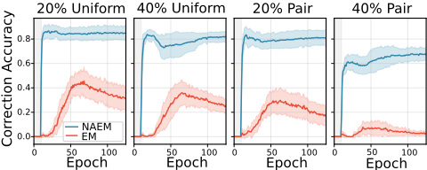
To verify NAEM recovers latent ground truth rather than overfitting, we monitor Correction Accuracy, which is defined as the accuracy of hard labels inferred from posterior q(Y ) against true labels on initially corrupted nodes. Figure 4 compares NAEM with Standard EM on AmazonPhotos. Standard EM displays a characteristic rise-and-fall pattern that peaks mid-training before degrading, signifying posterior collapse as the model overfits noisy supervision. Conversely, NAEM sustains high accuracy following a rapid ascent. Under 40% Pair Noise, NAEM maintains accuracy near 0.7, whereas the baseline remains below 0.1. This validates Neighborhood Agreement as a structural regularizer: by calibrating uncertainty via consensus, NAEM prevents posterior degeneration toward noise, enabling iterative refinement toward ground truth. Qualitatively, t-SNE visualization in Supplementary Sec. B.6 demonstrates that NAEM learns more compact, discriminative representations than baselines, aligning noisy nodes with true semantic clusters.
Noise Transition Matrix Estimation
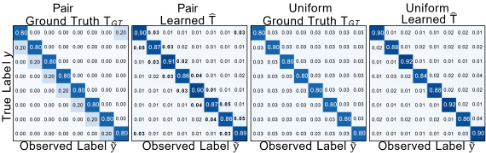
To validate whether NAEM can capture the underlying noise patterns, we compare the learned transition matrix ˆT with the ground truth TGT on the Amazon-Photos dataset under 20% Pair and Uniform noise. Figure 5 visualizes these matrices as heatmaps. For Pair noise, while NAEM underestimates the absolute noise magnitude, it correctly captures the structured pairwise flipping pattern via the dominant offdiagonal elements. Similarly, under uniform noise, the model successfully estimates the dispersed noise distribution. This ability to reconstruct the true noise dynamics allows NAEM to decouple corruption from semantic features, thereby explaining away systematic biases in the labels and ensuring robust learning. Sensitivity analyses for Ewarm, λNA, γ, τhigh, and τlow are provided in Supplementary Sec. B.7, confirming NAEM's robustness across broad hyperparameter settings.
5 Conclusion
We presented NAEM, a probabilistic framework that treats graph label denoising as latent variable inference rather than heuristic sample selection or indiscriminate smoothing. By integrating Neighborhood Agreement into EM, NAEM calibrates posterior uncertainty, mitigates topology-dependent noise propagation, and jointly estimates the noise transition matrix to disentangle corruption from semantic representations. Extensive experiments demonstrate consistent robustness under diverse noise settings. Future work will study open-set noise and broader heterophilic regimes.
Acknowledgments
This work was supported by the National Natural Science Foundation of China (No. U2433212), in part by the Fundamental Research Funds for the Central Universities, and in part by the State Key Laboratory of Complex & Critical Software Environment.
@inproceedings{ijcai2026p317,
  title     = {Graph Label Denoising via Neighborhood Agreement–Guided Expectation Maximization},
  author    = {Liu, Dezhi and Zhang, Richong and Chen, Junfan and Tian, Fengbo and Chen, Si},
  booktitle = {Proceedings of the Thirty-Fifth International Joint Conference on
               Artificial Intelligence, {IJCAI-26}},
  publisher = {International Joint Conferences on Artificial Intelligence Organization},
  editor    = {Diego Calvanese},
  pages     = {2852--2860},
  year      = {2026},
  month     = {8},
  note      = {Main Track},
  doi       = {10.24963/ijcai.2026/317},
  url       = {https://doi.org/10.24963/ijcai.2026/317},
}
TY - CPAPER TI - Graph Label Denoising via Neighborhood Agreement–Guided Expectation Maximization AU - Liu, Dezhi AU - Zhang, Richong AU - Chen, Junfan AU - Tian, Fengbo AU - Chen, Si T2 - Proceedings of the Thirty-Fifth International Joint Conference on Artificial Intelligence, IJCAI-26 PB - International Joint Conferences on Artificial Intelligence Organization PY - 2026 SP - 2852 EP - 2860 DO - 10.24963/ijcai.2026/317 UR - https://doi.org/10.24963/ijcai.2026/317 ER -Copied
Machine-readable versions of this paper, for tools and AI agents:





