
StreamTimer: Efficient Inference for Long-Context Time Series Transformers
Proceedings of the Thirty-Fifth International Joint Conference on Artificial Intelligence. Main Track. Pages 2942-2950.
https://doi.org/10.24963/ijcai.2026/327
Keywords
- Machine Learning: Time series and data streams
- Data Mining: Mining spatial and/or temporal data
Abstract
Time series forecasting (TSF) plays a vital role across various domains such as finance, energy, healthcare, and meteorology. Currently, most deep learning based TSF methods typically operate with a fixed lookback window. This approach comes from the high compute and memory costs of long contexts, as well as the standard practice of using sliding windows. This creates a trade-off. Making the window larger reduces the number of training samples, which can harm stability and generalization. However, keeping the window small prevents the model from using long history during inference. We propose an inference-only streaming autoregressive framework that replaces repeated full-context recomputation with a one-time context warmup and incremental decoding, enabling efficient long-history forecasting without retraining. While straightforward caching attentions is brittle for time series due to distribution shifts and noisy or redundant histories, we address these issues with cache-consistent normalization and selective memory under a fixed cache budget. Across diverse benchmarks, our approach substantially reduces inference latency with no or marginal accuracy loss, and often improves performance when longer lookbacks are beneficial.
- [Ansari and Stella, 2024] Abdul Fatir Ansari and Stella. Chronos: Learning the language of time series. Trans- actions on Machine Learning Research, 2024.
- [Chang et al., 2024] Ching Chang, Wei-Yao Wang, Wen- Chih Peng, and Tien-Fu Chen. Llm4ts: Aligning pre- trained llms as data-efficient time-series forecasters, 2024.
- [Fan et al., 2023] Wei Fan, Pengyang Wang, Dongkun Wang, Dongjie Wang, Yuanchun Zhou, and Yanjie Fu. Dish-ts: A general paradigm for alleviating distribution shift in time series forecasting. In Proceedings of the AAAI Conference on Artificial Intelligence, volume 37, pages 7522-7529, 2023.
- [Jin et al., 2024] Ming Jin, Shiyu Wang, Lintao Ma, Zhix- uan Chu, James Y. Zhang, Xiaoming Shi, Pin-Yu Chen, Yuxuan Liang, Yuan-Fang Li, Shirui Pan, and Qingsong Wen. Time-llm: Time series forecasting by reprogram- ming large language models, 2024.
- [Kim et al., 2021] Taesung Kim, Jinhee Kim, Yunwon Tae, Cheonbok Park, Jang-Ho Choi, and Jaegul Choo. Re- versible instance normalization for accurate time-series forecasting against distribution shift. In International Con- ference on Learning Representations, 2021.
- [Kudrat et al., 2025] Dilfira Kudrat, Zongxia Xie, Yanru Sun, Tianyu Jia, and Qinghua Hu. Patch-wise struc- tural loss for time series forecasting. In Aarti Singh, Maryam Fazel, Daniel Hsu, Simon Lacoste-Julien, Fe- lix Berkenkamp, Tegan Maharaj, Kiri Wagstaff, and Jerry Zhu, editors, Proceedings of the 42nd International Con- ference on Machine Learning, volume 267 of Proceed- ings of Machine Learning Research, pages 31841-31859. PMLR, 13-19 Jul 2025.
- [Lin et al., 2023] Shengsheng Lin, Weiwei Lin, Wentai Wu, Feiyu Zhao, Ruichao Mo, and Haotong Zhang. Segrnn: Segment recurrent neural network for long-term time se- ries forecasting, 2023.
- [Lin et al., 2024] Shengsheng Lin, Weiwei Lin, Wentai Wu, Haojun Chen, and Junjie Yang. Sparsetsf: Modeling long- term time series forecasting with 1k parameters. In Forty- first International Conference on Machine Learning, 2024.
- [Liu et al., 2023] Zhiding Liu, Mingyue Cheng, Zhi Li, Zhenya Huang, Qi Liu, Yanhu Xie, and Enhong Chen. Adaptive normalization for non-stationary time series forecasting: A temporal slice perspective. In Thirty- seventh Conference on Neural Information Processing Systems, 2023.
- [Liu et al., 2024a] Xu Liu, Juncheng Liu, Gerald Woo, Taha Aksu, Yuxuan Liang, Roger Zimmermann, Chenghao Liu, Silvio Savarese, Caiming Xiong, and Doyen Sa- hoo. Moirai-moe: Empowering time series foundation models with sparse mixture of experts. arXiv preprint arXiv:2410.10469, 2024.
- [Liu et al., 2024b] Yong Liu, Tengge Hu, Haoran Zhang, Haixu Wu, Shiyu Wang, Lintao Ma, and Mingsheng Long. itransformer: Inverted transformers are effective for time series forecasting, 2024.
- [Liu et al., 2024c] Yong Liu, Guo Qin, Xiangdong Huang, Jianmin Wang, and Mingsheng Long. Timer-xl: Long- context transformers for unified time series forecasting. arXiv preprint arXiv:2410.04803, 2024.
- [Liu et al., 2024d] Yong Liu, Haoran Zhang, Chenyu Li, Xi- angdong Huang, Jianmin Wang, and Mingsheng Long. Timer: Generative pre-trained transformers are large time series models. In Forty-first International Conference on Machine Learning, 2024.
- [Luo and Wang, 2024] Donghao Luo and Xue Wang. Mod- erntcn: A modern pure convolution structure for general time series analysis. In The Twelfth International Confer- ence on Learning Representations, 2024.
- [Makridakis et al., 2020] Spyros Makridakis, Evangelos Spiliotis, and Vassilios Assimakopoulos. The m4 compe- tition: 100,000 time series and 61 forecasting methods. International Journal of Forecasting, 36(1):54-74, 2020.
- [Muñoz-Sabater et al., 2021] Joaquín Muñoz-Sabater, Emanuel Dutra, Anna Agustí-Panareda, Clément Al- bergel, Gabriele Arduini, Gianpaolo Balsamo, Souhail Boussetta, Margarita Choulga, Shaun Harrigan, Hans Hersbach, et al. Era5-land: A state-of-the-art global reanalysis dataset for land applications. Earth system science data, 13(9):4349-4383, 2021.
- [Nie et al., 2023] Yuqi Nie, Nam H. Nguyen, Phanwadee Sinthong, and Jayant Kalagnanam. A time series is worth 64 words: Long-term forecasting with transformers. In The Eleventh International Conference on Learning Rep- resentations, ICLR 2023, Kigali, Rwanda, May 1-5, 2023. OpenReview.net, 2023.
- [Qiu et al., 2024] Xiangfei Qiu, Jilin Hu, Lekui Zhou, Xingjian Wu, Junyang Du, Buang Zhang, Chenjuan Guo, Aoying Zhou, Christian S. Jensen, Zhenli Sheng, and Bin Yang. Tfb: Towards comprehensive and fair benchmark- ing of time series forecasting methods, 2024.
- [Shi et al., 2025] Xiaoming Shi, Shiyu Wang, Yuqi Nie, Di- anqi Li, Zhou Ye, Qingsong Wen, and Ming Jin. Time- moe: Billion-scale time series foundation models with mixture of experts, 2025.
- [Wang et al., 2024a] Shiyu Wang, Haixu Wu, Xiaoming Shi, Tengge Hu, Huakun Luo, Lintao Ma, James Y. Zhang, and Jun Zhou. Timemixer: Decomposable multiscale mixing for time series forecasting. In The Twelfth International Conference on Learning Representations, ICLR 2024, Vi- enna, Austria, May 7-11, 2024. OpenReview.net, 2024.
- [Wang et al., 2024b] Yuxuan Wang, Haixu Wu, Jiaxiang Dong, Yong Liu, Mingsheng Long, and Jianmin Wang. Deep time series models: A comprehensive survey and benchmark. CoRR, abs/2407.13278, 2024.
- [Woo et al., 2024] Gerald Woo, Chenghao Liu, Akshat Ku- mar, Caiming Xiong, Silvio Savarese, and Doyen Sahoo. Unified training of universal time series forecasting trans- formers. In Forty-first International Conference on Ma- chine Learning, 2024.
- [Wu et al., 2024] Yuhan Wu, Xiyu Meng, Yang He, Junru Zhang, Haowen Zhang, Yabo Dong, and Dongming Lu. Multi-view self-supervised contrastive learning for multi- variate time series. In Proceedings of the 32nd ACM In- ternational Conference on Multimedia, pages 9582-9590, 2024.
- [Wu et al., 2025] Yuhan Wu, Xiyu Meng, Huajin Hu, Junru Zhang, Yabo Dong, and Dongming Lu. Affirm: Interac- tive mamba with adaptive fourier filters for long-term time series forecasting. In Toby Walsh, Julie Shah, and Zico Kolter, editors, AAAI-25, Sponsored by the Association for the Advancement of Artificial Intelligence, February 25 -March 4, 2025, Philadelphia, PA, USA, pages 21599- 21607. AAAI Press, 2025.
- [Xiao et al., 2024] Guangxuan Xiao, Yuandong Tian, Beidi Chen, Song Han, and Mike Lewis. Efficient streaming lan- guage models with attention sinks. In International Con- ference on Learning Representations (ICLR), 2024.
- [Zeng et al., 2023] Ailing Zeng, Muxi Chen, Lei Zhang, and Qiang Xu. Are transformers effective for time series fore- casting? In Brian Williams, Yiling Chen, and Jennifer Neville, editors, Thirty-Seventh AAAI Conference on Ar- tificial Intelligence, AAAI 2023, Thirty-Fifth Conference on Innovative Applications of Artificial Intelligence, IAAI 2023, Thirteenth Symposium on Educational Advances in Artificial Intelligence, EAAI 2023, Washington, DC, USA, February 7-14, 2023, pages 11121-11128. AAAI Press, 2023.
- [Zhang and Dong, 2025] Jiayu Zhang and Yuantong Dong. Multi-period normalization for long-term time series fore- casting. In ICASSP 2025 -2025 IEEE International Conference on Acoustics, Speech and Signal Processing (ICASSP), pages 1-5, 2025.
- [Zhou et al., 2021] Haoyi Zhou, Shanghang Zhang, Jieqi Peng, Shuai Zhang, Jianxin Li, Hui Xiong, and Wancai Zhang. Informer: Beyond efficient transformer for long sequence time-series forecasting. In Thirty-Fifth AAAI Conference on Artificial Intelligence, AAAI 2021, Thirty- Third Conference on Innovative Applications of Artificial Intelligence, IAAI 2021, The Eleventh Symposium on Ed- ucational Advances in Artificial Intelligence, EAAI 2021, Virtual Event, February 2-9, 2021, pages 11106-11115. AAAI Press, 2021.
- [Zhou et al., 2023] Tian Zhou, Peisong Niu, Xue Wang, Liang Sun, and Rong Jin. One fits all: Power general time series analysis by pretrained LM. In NeurIPS, 2023.
References were extracted automatically from the PDF and may contain errors.
Full text extracted automatically from the PDF; figures, tables and equations may differ. The PDF is the version of record.
1 Introduction
Long-term time series forecasting has evolved rapidly over the past decades, witnessing a paradigm shift from traditional statistical methods to deep learning architectures [Jin et al., 2024; Wang et al., 2024b]. While these substantial architectural innovations, their fundamental operational protocol remains surprisingly static, characterized by a reliance on a fixed lookback window [Qiu et al., 2024]. Specifically, models are constrained to a pre-determined number of historical time steps (e.g., 96 days or 720 hours) to forecast future values [Liu et al., 2024b]. This rigid sliding window approach persists even as underlying architectures grow increasingly complex, creating a misalignment between the model's intrinsic capacity and its effective utilization of context.
This operational rigidity introduces a paradox in modern TSF. That is, longer historical contexts theoretically harbor richer temporal information, but extending the window to capture it is computationally expensive. Given the quadratic complexity of self-attention, lengthening the window substantially increases memory and compute costs [Zhou et al., 2021]. Besides, empirical evidence suggests that simply enlarging the window often degrades performance due to attention dispersion, insufficient training samples, and overfitting to irrelevant noise [Nie et al., 2023; Liu et al., 2024d]. Consequently, practitioners are trapped in a dilemma: they must either truncate history or risk computational intractability and model instability. This suggests that the fixed-window paradigm is inherently suboptimal for capturing the continuous and unrestricted dynamics of time series data.
To resolve these structural limitations, we propose a transition from the repeated recomputation of fixed windows to an Inference-Only Streaming Autoregressive Framework. Inspired by the efficient caching mechanisms in Large Language Models (LLMs), our approach views forecasting as a continuous, stateful process. By replacing repeated fullcontext recomputation with a one-time context warmup followed by incremental decoding, we reduce the complexity of extending context from quadratic to linear. This allows the model to efficiently leverage extensive historical data without the latency penalties of massive fixed windows. Moreover, as an inference-time optimization, this framework requires no retraining, allowing the trained model to achieve superior long-context performance directly
However, the direct adaptation of NLP-style Key-Value (KV) caching [Xiao et al., 2024] to time series is brittle due to two domain challenges. First, time series data are non-stationary. Current baselines typically employ Reversible Instance Normalization (RevIN) [Kim et al., 2021; Qiu et al., 2024] to mitigate statistical drifts; however, this creates distribution cache mismatches, meaning that the key vectors stored at time t effectively reside in a different feature space than Query vectors generated at t + 1. Second, unlike semantically dense text, time series history is replete with redundancy, where indiscriminately caching noise diminishes the efficacy of the attention mechanism.
To overcome these issues, we introduce StreamTimer, a robust streaming framework tailored for TSF. We propose Cache-Consistent Normalization to dynamically align cached representations with the current statistical regime, and incorporate window attention with attention sinks to maintain temporal coherence while retaining only high-value historical tokens. Our contributions lie in three aspects:
- We propose the first inference-only streaming framework with Timer backbones for TSF that effectively utilizes the lookback window, decoupling context length from computational cost.
- We identify and resolve the normalization mismatch problem in generative trained large time series models, ensuring mathematically consistent distribution during streaming inference.
- Experiments validate that StreamTimer achieves significant speedup while outperforming SOTA baselines, particularly on ultra-long sequences.
2 RelatedWork
2.1 Time Series Forecasting
Contemporary deep learning architectures for time series forecasting predominantly focus on modeling complex global temporal dependencies and multivariate interactions from historical data. Early studies built on Recurrent Neural Networks [Lin et al., 2023] and Temporal Convolutional Networks [Luo and Wang, 2024] to capture local patterns through gated recurrences and dilated convolutions. More recently, Transformers have emerged as the mainstream for long-horizon forecasting due to their capability to capture long-range dependencies. Specifically, Informer [Zhou et al., 2021] introduces sparse attention tailored to long sequences, PatchTST [Nie et al., 2023] and iTransformer [Liu et al., 2024b] leverage patch- and channel-centric designs, and TimeMixer [Wang et al., 2024a] and TimeMoE [Shi et al., 2025] enhance the exploitation of multivariate structures and multi-scale temporal patterns. While these backbones provide robust representation capabilities, they typically rely on a fixed-lookback-fixed-forecast recomputation paradigm.
2.2 Generative Pre-training for Large Time Series Models
The field of TSF has transitioned from small-scale, taskspecific deep learning models [Wu et al., 2025; Lin et al., 2024; Wu et al., 2024; Zeng et al., 2023] to Large Time Series Models (LTSMs) [Zhou et al., 2023; Jin et al., 2024; Liu et al., 2024a; Woo et al., 2024; Ansari and Stella, 2024] powered by unsupervised pre-training on massive datasets. Inspired by the success of LLMs, recent works have explored generative pre-training paradigms to build foundation models for time series.
Early efforts, such as Time-LLM [Jin et al., 2024] and LLM4TS [Chang et al., 2024], repurposed pre-trained LLMs (e.g., LLaMA, GPT-2) by aligning time series modalities with textual tokens. However, these methods often suffer from high computational overhead due to cross-modality alignment. More recently, native LTSMs like Timer [Liu et al., 2024d] have emerged, employing a decoder-only Transformer architecture trained via next-token prediction on largescale heterogeneous datasets. Timer unifies various forecasting tasks into a single generative framework, demonstrating strong zero-shot generalization capabilities. Building on this, Timer-XL [Liu et al., 2024c] addresses the context bottleneck by introducing TimeAttention to capture fine-grained intraand inter-series dependencies, expanding the context window to thousands of tokens.
Despite these architectural advancements, both Timer and Timer-XL adhere to a recomputation-based inference protocol. To forecast a future horizon, these models require processing a fixed lookback window from scratch at each step. This rigid mechanism incurs quadratic computational complexity O(TL2 ) with respect to the context length L and the forecast horizon T, severely limiting their efficiency when handling extremely long historical contexts in real-time streaming scenarios.
3 Approach
3.1 Preliminaries
We construct our streaming framework upon the foundation of LTSMs, specifically adopting the decoder-only Transformer architecture employed by Timer [Liu et al., 2024d] and Timer-XL [Liu et al., 2024c]. Unlike traditional deep forecasters that rely on encoder-decoder structures, Timer and Timer-XL treat time series forecasting as a native sequence generation task.
Patch-basedTokenization. Given a rawunivariate time series X = {x1, . . . , xL} ∈ RL, the model first transforms the continuous data points into a sequence of discrete embeddings. We adopt a patching strategy where non-overlapping windows of size P are aggregated into tokens. The resulting sequence S = (s1, . . . , sN) consists of N = L/P tokens, where each st ∈ RP represents a local temporal segment. These segments are then projected into a high-dimensional latent space RD via a learnable linear embeddingWemb:
where PEt denotes the positional encoding required to preserve temporal ordering.
Causal Contextualization. The core computation occurs within a stack of K decoder-only Transformer blocks. To ensure the autoregressive property, a strict causal mask M is applied to the self-attention mechanism. For the k-th layer, the representation h(k) t is updated by attending solely to historical tokens:
where Mij = -∞ if j > i. This mechanism guarantees that the information flow at step t is strictly isolated from future signals.
Generative Objective. The training paradigm mirrors that of LLMs, formulating forecasting as a next token prediction (NTP) problem. The joint probability of the time series is factorized into a product of conditional probabilities:
In the continuous domain of time series, this probabilistic objective manifests as minimizing the reconstruction error between the predicted next patch and the ground truth. The model outputs the prediction ˆst+1 via a linear projection head
Whead applied to the final hidden state h(K) t . The optimization objective is defined as the Mean Squared Error (MSE) over the sequence:
Through this formulation, the model learns to synthesize future trajectories based on the unified history representations, establishing the theoretical basis for our subsequent streaming optimizations.
3.2 Hybrid-Scale Normalization for Patch-based Generators
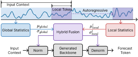
RevIN [Kim et al., 2021] effectively mitigates distribution shifts by normalizing the input using the mean and variance over the entire lookback window. However, for patch-based autoregressive models like Timer, relying solely on global statistics may overlook rapid and high-frequency fluctuations within individual patches. Conversely, normalizing strictly at the patch level risks discarding the global amplitude information necessary for accurate trajectory reconstruction.
To address this dilemma, we introduce a Hybrid-Scale Normalization strategy that dynamically calibrates the distribution by fusing global and local statistics. Let X ∈ RL×C denote the input lookback window with length L and C variables. We first compute the global statistics across the temporal dimension:
Simultaneously, for the i-th patch si ∈ RP×C , where P is the patch size, we compute its local statistics µ(i) local and σ(i) local .
To balance the stability of global trends with the sensitivity to local variations, we define the normalization statistics as a convex combination of both scales, controlled by a mixing coefficient α:˜µ(i) = α · µ(i)
Each input patch si is then normalized as ¯si = (si - ˜µ(i) )/˜σ(i) . Crucially, to ensure consistency, the generative output ˆsi is denormalized using the same hybrid statistics:
In our implementation, α is a learnable parameter initialized to 0.5. This design allows the model to remain robust to non-stationary drifts while retaining essential global context, thereby enhancing the generation stability of Timer and Timer-XL. We provide detailed empirical and theoretical verification of this choice in Appendix C.
3.3 Linear-Complexity Streaming via KVCaching
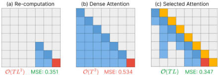
The standard inference paradigm of Transformers typically involves a recomputation strategy, where the entire history is processed repeatedly to generate the next token. For a sequence of length L, this results in a computational complexity of O(L2 ), rendering long-context forecasting prohibitively expensive. To address this, we implement a Streaming Inference Mechanism based on KV Caching, adapted for the patch-based architecture of Timer.
Mechanism. Instead of recalculating the representations of historical patches at every step, we cache the Key K and Value V matrices computed in previous iterations. Let st denote the input patch at step t. During the streaming process, the model only computes the Query qt, Key kt, and Value vt for the current patch. The attention mechanism then attends to the concatenation of the cached states and the current states:
Here, [·; ·] denotes concatenation along the temporal dimension. By maintaining this persistent memory state, the computation for the current step t becomes independent of the history length t - 1 in terms of feature extraction, involving only a single forward pass of the Transformer block.
Implementation Protocol. Operationally, we reformulate the inference process as a stateful autoregressive protocol over the discretized time horizon. The procedure commences by initializing an empty Key-Value memory. Unlike standard batch processing, the model subsequently enters a streaming phase where it ingests exclusively the current patch st at each time step t. During this incremental pass, the transformer blocks query the historical context persisted in the cache to derive the current representation yt, Crucially, to constrain memory growth, we employ an attention-based eviction policy: post-computation, we retain only the [REG] token serving as an attention sink and the subset of historical tokens with the highest attention scores. Low-scoring tokens are discarded from the memory bank. This selective retention strategy allows us to reconstruct the coherent forecast trajectory with a bounded memory overhead per step.
4 Experiments
We evaluate StreamTimer across three dimensions: (1) supervised training as a task-specific forecaster, (2) transfering as a zero-shot forecaster, and (3) the effectiveness of normalization and model efficiency. Since performance saturation on previous benchmarks [Qiu et al., 2024; Wang et al., 2024b] often conceals the challenges of the long-context forecasting paradigm, we establish new long-context forecasting benchmarks by following the experimental settings of TimerXL [Liu et al., 2024c]. Detailed experimental configurations are provided in Appendix A.
4.1 Univariate Time Series Forecasting
Setups To address the issue of data scarcity often encountered when extending context lengths in univariate time series [Makridakis et al., 2020], we follow the experimental protocol of Timer-XL [Liu et al., 2024c]. Specifically, we leverage the multivariate datasets from [Liu et al., 2024b] and formulate univariate forecasting tasks by applying channel independence. The core objective of our experiments is to evaluate model robustness given long historical inputs, rather than merely pursuing extended forecasting horizons. Consequently, we fix the forecast horizon and focus on expanding the lookback window to monthly and yearly scales. Furthermore, we establish a challenging long-context univariate benchmark named ERA5-S, derived from the ECMWF Reanalysis v5 (ERA5) dataset [Mu˜noz-Sabater et al., 2021]. Leveraging its 40-year temporal span, this benchmark is specifically designed to assess land-surface temperature forecasting capabilities based on yearly contexts.
Results As illustrated in Figure 3, increasing the context length generally leads to improved prediction accuracy across univariate datasets. While previous state-of-the-art models like Timer-XL show promising results, they tend to encounter performance saturation or even deterioration in excessively long contexts (e.g., monthly and yearly levels), likely due to the accumulation of noise. In contrast, our proposed StreamTimer exhibits superior robustness. As shown in the curves, StreamTimer consistently outperforms Timer-XL and DLinear, particularly achieving lower MSE in the longest lookback settings across all datasets. This indicates that StreamTimer effectively mitigates the impact of irrelevant history while capturing critical long-term dependencies. A similar conclusion can be drawn from the ERA5-S benchmark (Table 1), where StreamTimer surpasses both PatchTST and Timer-XL
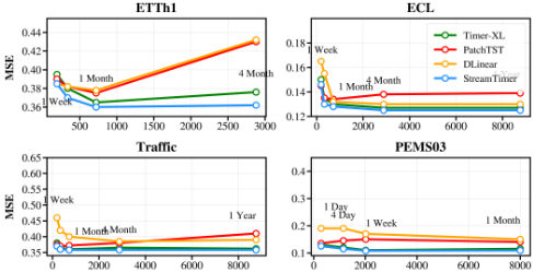
on all sites, demonstrating its efficacy in handling complex meteorological data with extended contexts.
Revisiting Non-stationary Forecasting We delve into the widespread non-stationarity in univariate tasks. While normalization techniques like RevIN [Kim et al., 2021] generally benefit Transformer performance by aligning statistical distributions, their limitations become pronounced in ultralong contexts. We argue that standard normalization oversimplifies the time-varying statistics inherent in long history. Specifically, as the context length increases, both the internal distribution shifts within the input and the statistical discrepancy between input and output are significantly exacerbated. Forcing such complex sequences into a unified distribution constrains the model capacity of Transformers. The model is compelled to handle these distorted distributions rather than learning distinct temporal variations, leading to side effects such as mode collapse and oversmoothed predictions. In contrast, our proposed normalization optimizes the distributional properties, thereby liberating the model's capacity to focus on the forecasting task itself rather than struggling with distribution alignment. As evidenced in Table 1, this approach allows Timer-XL and Timer to achieve superior results on ERA5-S without the pitfalls of standard normalization.
4.2 Multivariate Time Series Forecasting
Setups Following the experimental protocols of TimerXL [Liu et al., 2024b], we evaluate multivariate forecasting performance. To advance the development of generated transformers, we focus on the rolling forecast setting, where a single trained model adapts to various prediction horizons by recursively integrating previous predictions into the lookback window for the next iteration. Furthermore, we establish a long-context multivariate benchmark, the ERA5 multistation land-surface temperature prediction (ERA5-MS). This benchmark is designed to facilitate the learning of complex temporal dynamics and inter-variable correlations with sufficient training samples.
Results As shown in Table 2, StreamTimer achieves the best results on the established benchmarks. Our comparison focuses primarily on its predecessors, Timer and Timer-XL.
| Station | Beijing | Hongkong | London | New York | Paris | Seoul | Shanghai | Average | ||||||||
|---|---|---|---|---|---|---|---|---|---|---|---|---|---|---|---|---|
| Model | MSE | MAE | MSE | MAE | MSE | MAE | MSE | MAE | MSE | MAE | MSE | MAE | MSE | MAE | MSE | MAE |
| Timer | 0.076 | 0.212 | 0.189 | 0.321 | 0.277 | 0.414 | 0.185 | 0.332 | 0.262 | 0.413 | 0.090 | 0.227 | 0.136 | 0.285 | 0.174 | 0.315 |
| + RevIN | 0.076 | 0.211 | 0.192 | 0.324 | 0.277 | 0.415 | 0.187 | 0.334 | 0.268 | 0.409 | 0.090 | 0.227 | 0.137 | 0.285 | 0.175 | 0.315 |
| + Ours | 0.073 | 0.208 | 0.181 | 0.315 | 0.269 | 0.409 | 0.182 | 0.330 | 0.261 | 0.408 | 0.087 | 0.224 | 0.130 | 0.278 | 0.169 | 0.310 |
| Timer-XL | 0.074 | 0.210 | 0.179 | 0.316 | 0.262 | 0.404 | 0.182 | 0.327 | 0.254 | 0.399 | 0.090 | 0.229 | 0.134 | 0.282 | 0.168 | 0.310 |
| + RevIN | 0.074 | 0.210 | 0.183 | 0.317 | 0.278 | 0.418 | 0.181 | 0.330 | 0.264 | 0.407 | 0.090 | 0.227 | 0.133 | 0.281 | 0.172 | 0.313 |
| + Ours | 0.073 | 0.208 | 0.173 | 0.312 | 0.260 | 0.403 | 0.180 | 0.317 | 0.251 | 0.396 | 0.088 | 0.224 | 0.130 | 0.279 | 0.165 | 0.306 |
| Models | StreamTimer (Ours) | Timer-XL (2025) | Timer (2024) | UniTST (2024) | iTransformer (2023) | DLinear (2023) | PatchTST (2022) | TimesNet (2022) | Stationary (2022) | Autoformer (2011) | |||||||||||||||||
|---|---|---|---|---|---|---|---|---|---|---|---|---|---|---|---|---|---|---|---|---|---|---|---|---|---|---|---|
| Metric | MSE | MAE | MSE | MAE | MSE | MAE | MSE | MAE | MSE | MAE | MSE | MAE | MSE | MAE | MSE | MAE | MAE | MSE | MSE | MAE | |||||||
| ETTh1 | 96 192 336 | 0.347 0.376 0.389 | 0.387 0.407 0.417 | 0.364 0.405 0.427 | 0.397 0.424 0.439 | 0.371 0.407 0.434 0.461 | 0.404 0.429 0.445 0.466 | 0.379 0.415 0.440 0.482 | 0.415 0.438 0.454 0.482 | 0.387 0.416 0.434 0.447 | 0.418 0.437 0.450 | 0.369 0.405 0.435 | 0.400 0.422 0.445 | 0.373 0.405 0.423 0.508 | 0.403 0.425 0.440 | 0.452 0.474 0.493 | 0.463 0.477 | 0.452 0.484 0.511 | 0.478 0.510 0.522 | 0.467 0.492 0.519 | 0.499 0.523 | 0.589 | |||||
| 720 Avg 96 | 0.399 0.378 0.275 | 0.434 0.411 0.339 0.376 0.407 | 0.439 0.409 0.277 0.348 0.375 0.409 0.352 0.290 0.337 0.374 0.437 | 0.459 0.430 0.343 0.391 0.418 0.458 0.402 0.341 0.369 0.392 0.428 | 0.418 0.285 0.365 0.412 0.468 0.382 0.281 0.330 0.367 0.432 | 0.436 0.344 0.400 0.440 0.487 0.418 0.338 0.368 0.393 0.433 | 0.429 0.343 0.376 0.399 0.419 0.384 0.289 0.332 0.365 0.421 | 0.447 0.398 0.420 0.435 0.457 0.428 0.348 0.375 0.397 0.431 0.388 | 0.421 0.304 0.372 0.418 0.463 0.389 0.311 0.353 0.387 0.452 | 0.473 0.445 0.362 0.407 0.440 0.476 0.421 0.365 0.390 0.411 0.445 | 0.493 0.426 0.305 0.412 0.527 0.830 0.518 | 0.653 0.493 0.350 0.368 0.387 0.419 0.381 0.263 | 0.445 0.444 0.412 0.371 0.289 0.439 0.360 0.508 0.389 0.398 0.359 | 0.471 0.435 0.347 0.393 0.420 0.440 0.400 0.346 0.372 0.394 0.426 | 0.560 0.495 0.340 0.402 0.307 0.285 0.337 0.329 0.366 0.363 0.419 0.421 | 0.489 0.534 0.491 0.452 0.462 0.414 0.338 0.371 0.410 0.478 | 0.571 0.543 0.505 0.513 0.348 0.408 | 0.403 0.448 0.457 0.476 0.446 0.414 0.482 | 0.358 0.435 0.454 0.479 0.431 0.466 0.504 0.574 0.596 0.535 0.255 0.279 0.331 0.413 | 0.531 0.560 0.528 0.374 0.397 0.414 0.452 | 0.517 | ||||||
| ETTh2 | 192 336 720 Avg 96 192 336 720 Avg 96 192 336 | 0.336 0.356 0.401 | 0.359 0.175 0.242 0.293 0.127 0.145 0.159 0.187 0.155 0.340 | 0.382 0.257 0.301 0.337 0.246 0.238 0.247 0.256 | 0.352 0.175 0.239 0.293 0.161 0.348 0.369 | 0.383 0.257 0.301 0.342 0.251 0.240 0.250 0.260 | 0.352 0.171 0.228 0.282 0.163 0.359 0.373 | 0.260 0.230 0.336 0.306 0.225 0.244 0.262 0.297 | 0.376 0.183 0.250 0.311 0.168 0.205 0.164 0.353 | 0.403 0.272 0.315 0.356 0.229 0.258 0.262 0.294 0.258 | 0.165 0.399 0.409 | 0.265 | 0.311 0.361 0.169 0.359 0.377 | 0.385 0.259 0.299 0.331 0.268 0.255 0.265 | 0.357 0.349 0.167 0.172 0.230 0.233 0.298 0.280 0.228 0.201 | 0.468 0.427 0.375 0.387 0.411 0.450 0.399 0.406 0.187 0.249 0.321 | 0.424 0.448 0.407 0.414 0.524 0.541 0.497 0.578 0.509 0.514 0.475 0.237 0.306 0.330 0.387 0.404 0.424 0.525 0.486 0.374 | 0.399 0.358 0.322 0.346 | 0.289 | 0.451 0.475 0.492 0.454 0.466 0.496 0.530 0.558 0.512 0.267 0.339 0.309 0.335 0.351 | 0.374 | ||||||
| 720 192 336 96 192 336 720 | 0.341 0.358 0.374 0.412 0.371 | 0.241 0.251 0.275 0.251 | 0.376 0.360 0.377 0.418 | 0.390 0.236 0.252 0.279 | 0.392 0.148 0.164 0.388 0.431 | 0.407 0.239 0.256 0.285 0.259 | 0.380 0.150 0.166 0.386 | 0.398 0.257 0.250 0.257 | 0.417 0.158 0.373 0.386 | 0.419 0.259 0.267 0.275 | 0.422 0.461 | 0.285 | 0.446 0.251 0.268 0.393 | 0.382 0.250 0.272 0.276 0.305 | 0.432 0.357 0.152 0.151 0.167 0.171 0.593 0.596 0.600 | 0.497 0.192 0.200 0.303 0.315 0.317 0.319 | 0.265 0.610 0.626 0.633 | 0.352 | 0.403 0.295 0.303 0.403 0.379 0.412 0.423 0.440 | 0.282 0.289 | 0.291 0.290 | 0.450 | |||||
| ETTm1 ETTm2 ECL | Avg 96 720 Avg Avg | 0.342 0.275 0.322 0.358 0.416 0.343 0.166 0.228 0.283 0.368 0.261 0.125 0.141 0.152 0.177 0.149 0.148 | 0.445 0.392 0.335 0.365 0.388 0.422 0.378 0.256 0.288 0.330 0.387 0.315 0.218 0.233 0.246 0.270 0.242 | 0.271 0.374 | 0.322 0.219 0.277 0.255 | 0.275 0.129 0.201 0.384 0.151 | 0.327 0.221 0.289 0.202 0.245 | 0.265 0.130 0.206 0.421 | 0.290 0.133 | 0.340 0.296 0.274 | 0.423 | 0.319 0.298 | 0.345 0.238 0.302 0.436 0.391 | 0.318 0.232 0.318 0.275 | 0.282 0.261 0.138 0.132 0.203 0.222 0.619 0.602 | 0.314 0.184 0.335 0.322 | 0.630 | 0.366 0.347 | 0.333 0.288 0.357 0.376 0.379 0.325 0.457 0.433 | 0.185 0.305 | 0.320 0.256 0.320 | 0.374 | |||||
| 0.236 | 0.169 | 0.290 0.297 | |||||||||||||||||||||||||
| 0.157 | 0.205 | 0.265 | 0.425 | 0.185 | 0.241 | ||||||||||||||||||||||
| Traffic | 0.200 0.238 | 0.206 0.259 0.337 | 0.250 0.291 0.344 | 0.196 0.249 | 0.288 | 0.385 | 0.286 0.206 | 0.229 | 0.149 | 0.202 | 0.228 0.269 | 0.421 | |||||||||||||||
| Weather | 96 | 0.191 0.241 0.311 Avg 0.223 96 0.159 | 0.335 0.263 0.216 0.236 | 0.240 0.162 0.187 | 0.273 0.221 | 0.330 0.232 | 0.344 0.270 0.212 0.230 0.232 0.246 0.237 | 0.152 0.198 0.251 0.322 | 0.265 0.249 | 0.385 0.174 | 0.225 0.268 | 0.211 0.258 | 0.268 0.306 0.362 | 0.194 0.244 0.317 | 0.245 | 0.169 0.222 0.290 0.376 | 0.308 0.199 0.243 | 0.651 0.286 0.323 0.436 | 0.675 0.679 0.688 0.693 0.684 0.355 | 0.409 0.450 0.465 0.496 | 0.325 | ||||||
| Solar-Energy | 720 Avg | 336 0.203 0.233 | 0.279 0.251 0.276 | 0.205 0.238 | 0.239 0.255 0.279 | 0.252 0.233 | 0.253 0.266 0.249 | 0.250 0.292 0.241 | 0.291 | 0.227 0.290 0.374 0.266 0.183 0.205 0.224 0.239 | 0.309 0.360 0.291 0.265 | 0.239 0.193 0.214 0.233 | 0.258 0.274 0.291 | 0.168 0.189 0.212 0.240 | 0.285 0.329 0.268 0.264 0.237 0.180 0.257 0.199 0.277 0.220 0.305 | 0.321 0.295 | 0.310 0.254 | 0.264 | 0.272 0.326 | 0.347 | 0.452 | ||||||
| 192 336 720 | 0.245 | 0.198 | 0.249 | 0.231 0.190 0 | 0.340 0.272 0.240 | 0.213 0 | 0.246 | 0.307 | 0.291 0.202 | 0.269 | 0.320 0.226 | 0.401 0.287 0.368 0.377 | 0.401 0.329 | 0.513 0.435 0.206 | |||||||||||||
| 0.275 | 0.291 | 0.251 | 0.339 0.315 | 0.455 0.296 0.328 0.330 0.347 | |||||||||||||||||||||||
| 0.222 | 0.283 | 0.213 | 0.325 | ||||||||||||||||||||||||
| 0 | 1 | 0 | |||||||||||||||||||||||||
| 192 | 0.183 0.195 36 | 33 | 1 | 0 | 0.223 | 0.264 0.283 0.311 | 0.283 0.299 0.316 | 0.290 | 0.265 0 | 0 | |||||||||||||||||
| 3 | 0 | 0 | 0 | 0.307 0.254 | |||||||||||||||||||||||
| 2 | 0 | 0 | 1 | 3 | 0.322 | ||||||||||||||||||||||
| 1st | |||||||||||||||||||||||||||
| Count | |||||||||||||||||||||||||||
| 0.310 0.364 0.293 0.272 0.286 0.301 | |||||||||||||||||||||||||||
While Timer-XL already demonstrates strong capabilities over Timer by leveraging extended contexts, StreamTimer pushes the performance boundary even further. It is particularly noteworthy that StreamTimer significantly outperforms Timer-XL, especially on non-stationary time series (improving by 8.2% in ETTh1). We attribute this substantial improvement over Timer-XL to two key innovations: first, our proposed normalization effectively resolves the distribution shift issues that hinder Timer-XL in ultra-long contexts; second, the streaming forecasting mechanism enhances stability during continuous inference. Furthermore, we find StreamTimer achieves 69 wins out of 80 tests under different metrics and conditions, and maintains strong performance even on lowdimensional datasets with low predictability (e.g., ETT), underscoring its effectiveness and superiority.
| Model | Beijing | Hongkong | London | NewYork | Paris | Seoul | Shanghai | Average | ||||||
|---|---|---|---|---|---|---|---|---|---|---|---|---|---|---|
| MSE | MAE MSE | MAE | MSE | MAE | MSE | MAE | MSE | MAE | MSE | MAE | MSE | MAE MSE | MAE | |
| PatchTST | 0.0815 | 0.222 0.190 | 0.326 | 0.275 | 0.414 | 0.185 | 0.333 | 0.265 | 0.407 | 0.0977 | 0.240 | 0.139 | 0.290 0.176 | 0.319 |
| UniTST | 0.0753 | 0.213 0.179 | 0.318 | 0.269 | 0.410 | 0.185 | 0.330 | 0.256 | 0.401 | 0.0901 | 0.230 | 0.135 | 0.284 0.170 | 0.312 |
| Timer | 0.0734 | 0.210 0.182 | 0.319 | 0.268 | 0.407 | 0.183 | 0.329 | 0.255 | 0.399 | 0.0877 | 0.226 | 0.132 | 0.281 0.169 | 0.310 |
| Timer-XL | 0.0736 | 0.209 0.174 | 0.309 | 0.263 | 0.404 | 0.182 | 0.327 | 0.252 | 0.396 | 0.0872 | 0.225 | 0.130 | 0.278 0.166 | 0.307 |
| StreamTimer | 0.0732 | 0.207 0.172 | 0.306 | 0.260 | 0.401 | 0.181 | 0.325 | 0.251 | 0.394 | 0.0868 | 0.223 | 0.130 | 0.277 0.165 | 0.304 |
| Models | Timer | Timer-XL | |||||||||||||||||||
|---|---|---|---|---|---|---|---|---|---|---|---|---|---|---|---|---|---|---|---|---|---|
| +RevIN | +SAN | +Dish-TS | +MPNorm | +Ours | +RevIN | +SAN | +Dish-TS | +MPNorm | +Ours | ||||||||||||
| Metric | MSE | MAE | MSE | MAE | MSE | MAE | MSE | MAE | MSE | MAE | MSE | MAE | MSE | MAE | MSE | MAE | MSE | MAE | MSE | MAE | |
| 96 | 0.371 | 0.404 | 0.363 | 0.399 | 0.363 | 0.396 | 0.361 | 0.397 | 0.347 | 0.387 | 0.364 | 0.397 | 0.370 | 0.401 | 0.423 | 0.455 | 0.368 | 0.401 | 0.352 | 0.392 | |
| ETTh1 | 192 | 0.407 | 0.429 | 0.395 | 0.418 | 0.400 | 0.418 | 0.396 | 0.422 | 0.378 | 0.405 | 0.405 | 0.424 | 0.412 | 0.427 | 0.490 | 0.496 | 0.397 | 0.422 | 0.380 | 0.410 |
| 336 | 0.434 | 0.445 | 0.416 | 0.430 | 0.425 | 0.435 | 0.411 | 0.426 | 0.392 | 0.421 | 0.427 | 0.439 | 0.444 | 0.447 | 0.542 | 0.529 | 0.422 | 0.445 | 0.393 | 0.421 | |
| 720 | 0.461 | 0.466 | 0.456 | 0.464 | 0.451 | 0.458 | 0.454 | 0.462 | 0.398 | 0.433 | 0.439 | 0.459 | 0.472 | 0.475 | 0.663 | 0.614 | 0.447 | 0.451 | 0.403 | 0.437 | |
| Avg | 0.418 | 0.436 | 0.407 | 0.428 | 0.410 | 0.427 | 0.405 | 0.427 | 0.382 | 0.416 | 0.409 | 0.430 | 0.424 | 0.438 | 0.530 | 0.523 | 0.409 | 0.430 | 0.382 | 0.415 | |
| 96 | 0.151 | 0.202 | 0.158 | 0.210 | 0.158 | 0.211 | 0.157 | 0.210 | 0.149 | 0.201 | 0.157 | 0.205 | 0.157 | 0.210 | 0.161 | 0.220 | 0.156 | 0.208 | 0.152 | 0.201 | |
| 192 | 0.196 | 0.245 | 0.203 | 0.252 | 0.204 | 0.254 | 0.196 | 0.249 | 0.194 | 0.240 | 0.206 | 0.250 | 0.202 | 0.251 | 0.214 | 0.267 | 0.200 | 0.248 | 0.196 | 0.243 | |
| Weather | 336 | 0.249 | 0.288 | 0.250 | 0.289 | 0.257 | 0.294 | 0.248 | 0.286 | 0.244 | 0.287 | 0.259 | 0.291 | 0.248 | 0.288 | 0.270 | 0.311 | 0.247 | 0.286 | 0.245 | 0.281 |
| 720 | 0.330 | 0.344 | 0.313 | 0.335 | 0.331 | 0.347 | 0.318 | 0.341 | 0.312 | 0.339 | 0.337 | 0.344 | 0.312 | 0.335 0.343 | 0.367 | 0.313 | 0.336 | 0.314 | 0.330 | ||
| Avg | 0.232 | 0.270 | 0.231 | 0.271 | 0.237 | 0.276 | 0.230 | 0.271 | 0.225 | 0.267 | 0.240 | 0.272 | 0.230 | 0.271 | 0.247 | 0.291 | 0.229 | 0.270 | 0.227 | 0.264 | |
Performance on ERA5-MS To evaluate the model's capability in multivariate time series forecasting, we conducted experiments on the real-world ERA5-MS benchmark as shown in Table 3. We compared StreamTimer with strong baselines ranging from channel-independent approaches PatchTST, UniTST to large-scale generative models Timer, Timer-XL. The results indicate that StreamTimer effectively combines the benefits of advanced tokenization and architectural design, surpassing the Timer-XL. By consistently achieving the best metrics in both MSE and MAE across diverse stations, StreamTimer proves to be the most effective solution for multivariate forecasting in this setting.
| Task | StreamTimer | Timer-XL | Timer | PatchTST | ||||
|---|---|---|---|---|---|---|---|---|
| MSE | MAE | MSE | MAE | MSE | MAE | MSE | MAE | |
| ETTh1→ETTh2 | 0.345 | 0.388 | 0.367 | 0.398 | 0.354 | 0.385 | 0.386 | 0.400 |
| ETTh1→ETTm2 | 0.273 | 0.344 | 0.302 | 0.361 | 0.277 | 0.347 | 0.314 | 0.360 |
| ETTh2→ETTh1 | 0.485 | 0.485 | 0.508 | 0.499 | 0.588 | 0.537 | 0.565 | 0.509 |
| ETTh2→ETTm2 | 0.282 | 0.342 | 0.303 | 0.357 | 0.285 | 0.347 | 0.289 | 0.345 |
| ETTm1→ETTh2 | 0.377 | 0.412 | 0.402 | 0.429 | 0.395 | 0.415 | 0.447 | 0.434 |
| ETTm1→ETTm2 | 0.231 | 0.294 | 0.268 | 0.324 | 0.235 | 0.297 | 0.258 | 0.311 |
| ETTm2→ETTh2 | 0.354 | 0.394 | 0.358 | 0.396 | 0.394 | 0.410 | 0.411 | 0.418 |
| ETTm2→ETTm1 | 0.481 | 0.455 | 0.483 | 0.446 | 0.477 | 0.459 | 0.530 | 0.470 |
Zero Shot Forecasting Results To evaluate the generalization capability of StreamTimer on unseen datasets, we conducted zero-shot forecasting experiments. Following previous protocols [Jin et al., 2024; Kudrat et al., 2025], we selected ETTh1, ETTh2, ETTm1, and ETTm2 as source datasets and performed direct inference on the remaining datasets as targets. Table 5 presents the results for a prediction horizon of 192, where StreamTimer demonstrates consistent superiority across transfer tasks, significantly outperforming PatchTST and the baseline models, Timer and Timer-XL. This robustness across different granularities and domains is primarily attributed to StreamTimer's streaming dynamic adaptation mechanism. This mechanism enables the model to keenly capture and adapt to the distribution evolution of the target domain during the inference phase, thereby effectively mitigating the distribution shift challenges between the source and unseen target domains.
Ablation onHybrid-scaleNormalization To verify the effectiveness of our proposed normalization strategy, we conducted a comprehensive ablation study comparing it with several state-of-the-art normalization techniques, including RevIN [Kim et al., 2021], SAN [Liu et al., 2023], DishTS [Fan et al., 2023], and MPNorm [Zhang and Dong, 2025]. Table 4 reports the results on ETTh1 and Weather datasets using both Timer and Timer-XL as backbones. The results demonstrate that our proposed module consistently achieves the lowest MSE and MAE across almost all prediction lengths. While RevIN and MPNorm serve as strong baselines, our method further boosts performance, particularly on the ETTh1 dataset where non-stationarity is significant. Notably, while SAN and Dish-TS employ model-based statistics prediction that necessitates complex pre-processing and auxiliary modules, this added complexity yields negligible performance gains.
Ablation on KV Cache As shown in Table 6, our ablation study uncovers that RevIN induces severe distribution shift during KV cache streaming. Specifically, RevIN's error rises markedly as the horizon extends to 720, reflecting its failure to manage statistical variations in long streams. On the contrary, our method maintains a stable and low MSE, verifying that it causes almost no harm to model performance in streaming scenarios.
| Backbone | Timer | Timer-XL | |||||||
|---|---|---|---|---|---|---|---|---|---|
| Normalization | + RevIN | + Ours | + RevIN | + Ours | |||||
| Dataset | Horizon | MSE | MAE | MSE | MAE | MSE | MAE | MSE | MAE |
| ETTh1 | 196 | 0.420 | 0.439 | 0.377 0.389 | 0.407 | 0.425 | 0.441 | 0.382 | 0.412 |
| 336 | 0.462 | 0.478 | 0.417 | 0.456 | 0.477 | 0.392 | 0.424 | ||
| 720 | 0.524 | 0.540 | 0.399 | 0.434 | 0.531 | 0.547 | 0.403 | 0.438 | |
| Weather | 196 | 0.238 | 0.275 | 0.194 0.245 | 0.240 | 0.241 | 0.274 | 0.195 | 0.242 |
| 336 | 0.383 | 0.365 | 0.285 | 0.391 | 0.370 | 0.244 | 0.280 | ||
| 720 | 0.491 | 0.430 | 0.312 | 0.339 | 0.485 | 0.427 | 0.311 | 0.333 | |
4.3 Model Analysis
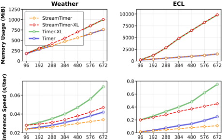
Model Efficiency To comprehensively evaluate model efficiency, it is essential to consider the input context length T, the number of variables N, and crucially, the prediction horizon L. Unlike 1D sequences, the computational overhead in multivariate time series forecasting is dictated by the interplay of these three dimensions. We provide a theoretical complexity analysis comparing StreamTimer against the baseline models, Timer and Timer-XL. Specifically, the complexity of Timer, which adopts channel independence, scales as O(NT 2L). Meanwhile, Timer-XL, which incorporates channel dependence to capture inter-variable correlations, sees its complexity escalate to O(N 2T 2L). Crucially, the computational burden of both architectures involves a multiplicative coupling with the prediction horizon L and quadratic terms of T, leading to significant overhead accumulation in longterm forecasting scenarios. In contrast, leveraging the streaming forecasting mechanism, StreamTimer effectively avoids the redundant re-computation of Keys and Values. As derived in Table 10, StreamTimer significantly optimizes the overall complexity to O(NTL). This indicates that the computational cost of StreamTimer scales linearly with the total sequence length, rather than multiplicatively. As shown in Figure 4, by eliminating these redundant operations, StreamTimer demonstrates an order-of-magnitude efficiency advantage, particularly in tasks involving extensive contexts and extended prediction horizons.
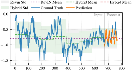
Visualization of Hybrid-Scale Normalization Figure 5 visualizes the effectiveness of the proposed normalization strategy. The blue and orange solid lines represent the ground truth and the model prediction, respectively. While RevIN relies on a static global mean (purple dotted line), which fails to capture temporal variations, our Hybrid-Scale Normalization utilizes local means (green and red dashed lines) that dynamically track local trends. Specifically, the red dashed line indicates that the model successfully infers the future distribution mean based on historical patterns. The alignment between the local statistics and the actual data demonstrates the method's precision in mitigating the impact of non-stationarity.
5 Conclusions
In this paper, we propose StreamTimer, a streaming inference framework designed to address the limitations of fixed lookback windows in time series forecasting. By reformulating the forecasting process into a continuous state update mechanism, we effectively leverage extremely long historical information without incurring additional computational burden. Our core technical innovations-particularly Cache-Consistent Normalization tailored for non-stationary data-effectively overcome the domain-specific barriers to applying KV caching in time series. Extensive experiments validate the efficiency of StreamTimer, demonstrating substantial reductions in both computational and memory costs while matching or even exceeding predictive performance. These results prove that decoupling context length from computational cost via streaming is both feasible and efficient, paving a new direction for the development of ultra-long sequence modeling and Time Series Foundation Models.
Acknowledgments
This work was supported in part by the Zhejiang Provincial Science and Technology Plan Project under Grant 2024C03261 and in part by Key Scientific Research Base for Digital Conservation of Cave Temples(Zhejiang University), National Cultural Heritage Administration.
Contribution Statement
Xiyu Meng and Yuhan Wu contributed equally to this work. Yabo Dong is the corresponding author.
@inproceedings{ijcai2026p327,
  title     = {StreamTimer: Efficient Inference for Long-Context Time Series Transformers},
  author    = {Meng, Xiyu and Wu, Yuhan and Xiao, Canran and Dong, Yabo and Xu, Duanqing},
  booktitle = {Proceedings of the Thirty-Fifth International Joint Conference on
               Artificial Intelligence, {IJCAI-26}},
  publisher = {International Joint Conferences on Artificial Intelligence Organization},
  editor    = {Diego Calvanese},
  pages     = {2942--2950},
  year      = {2026},
  month     = {8},
  note      = {Main Track},
  doi       = {10.24963/ijcai.2026/327},
  url       = {https://doi.org/10.24963/ijcai.2026/327},
}
TY - CPAPER TI - StreamTimer: Efficient Inference for Long-Context Time Series Transformers AU - Meng, Xiyu AU - Wu, Yuhan AU - Xiao, Canran AU - Dong, Yabo AU - Xu, Duanqing T2 - Proceedings of the Thirty-Fifth International Joint Conference on Artificial Intelligence, IJCAI-26 PB - International Joint Conferences on Artificial Intelligence Organization PY - 2026 SP - 2942 EP - 2950 DO - 10.24963/ijcai.2026/327 UR - https://doi.org/10.24963/ijcai.2026/327 ER -Copied
Machine-readable versions of this paper, for tools and AI agents:





