
Multi-View Ensemble for Time Series Anomaly Detection via Coupling Flows
Proceedings of the Thirty-Fifth International Joint Conference on Artificial Intelligence. Main Track. Pages 2988-2996.
https://doi.org/10.24963/ijcai.2026/332
Keywords
- Data Mining: Mining spatial and/or temporal data
Abstract
Time series anomaly detection faces a critical challenge that different anomaly types require different detection mechanisms, yet single methods are inherently limited by their design biases. We propose FlowFuse, a multi-view ensemble framework with coupling flow-based score fusion for time series anomaly detection. FlowFuse combines four complementary detection modules spanning temporal and frequency domains, as well as clustering and reconstruction paradigms, to extract multi-perspective anomaly scores. Rather than simple averaging, an ensemble of coupling flows models the joint distribution of these multi-view scores, learning complex inter-view dependencies through invertible transformations with alternating updates between temporal and frequency scores. The ensemble naturally quantifies detection uncertainty through prediction disagreement, which can optionally guide selective supervision when labels are available. Extensive experiments across 18 diverse benchmarks show that FlowFuse achieves state-of-the-art performance, demonstrating effectiveness across multiple anomaly types.
- [Bhatnagar et al., 2021] Aadyot Bhatnagar, Paul Kassianik, Chenghao Liu, Tian Lan, Wenzhuo Yang, Rowan Cassius, Doyen Sahoo, Devansh Arpit, Sri Subramanian, Gerald Woo, Amrita Saha, Arun Kumar Jagota, Gokulakrishnan Gopalakrishnan, Manpreet Singh, K C Krithika, Sukumar Maddineni, Daeki Cho, Bo Zong, Yingbo Zhou, Caiming Xiong, Silvio Savarese, Steven Hoi, and Huan Wang. Mer- lion: A machine learning library for time series. 2021.
- [Breunig et al., 2000] Markus M Breunig, Hans-Peter Kriegel, Raymond T Ng, and Jörg Sander. Lof: iden- tifying density-based local outliers. In Proceedings of the 2000 ACM SIGMOD international conference on Management of data, pages 93-104, 2000.
- [Campos et al., 2022] David Campos, Tung Kieu, Chenjuan Guo, Feiteng Huang, Kai Zheng, Bin Yang, and Chris- tian S. Jensen. Unsupervised time series outlier detec- tion with diversity-driven convolutional ensembles. Proc. VLDB Endow., 15(3):611-623, 2022.
- [Chandola et al., 2009] Varun Chandola, Arindam Banerjee, and Vipin Kumar. Anomaly detection: A survey. ACM computing surveys, 41(3):1-58, 2009.
- [Feng et al., 2021] Hsin-Yu Feng, Po-Ying Chen, and Janpu Hou. Sr-scatnet algorithm for on-device ecg time series anomaly detection. In SoutheastCon 2021, pages 1-5. IEEE, 2021.
- [Goldstein and Dengel, 2012] Markus Goldstein and An- dreas Dengel. Histogram-based outlier score (hbos): A fast unsupervised anomaly detection algorithm. KI-2012: poster and demo track, 1:59-63, 2012.
- [Guo et al., 2014] Chenjuan Guo, Christian S Jensen, and Bin Yang. Towards total traffic awareness. ACM SIGMOD Record, 43(3):18-23, 2014.
- [He et al., 2003] Zengyou He, Xiaofei Xu, and Shengchun Deng. Discovering cluster-based local outliers. Pattern recognition letters, 24(9-10):1641-1650, 2003.
- [Huang et al., 2022] Xuanwen Huang, Yang Yang, Yang Wang, Chunping Wang, Zhisheng Zhang, Jiarong Xu, Lei Chen, and Michalis Vazirgiannis. Dgraph: A large-scale financial dataset for graph anomaly detection. In NeurIPS, pages 22765-22777, 2022.
- [Huet et al., 2022] Alexis Huet, Jose Manuel Navarro, and Dario Rossi. Local evaluation of time series anomaly de- tection algorithms. In SIGKDD, pages 635-645, 2022.
- [Hundman et al., 2018] Kyle Hundman, Valentino Con- stantinou, Christopher Laporte, Ian Colwell, and Tom Soderstrom. Detecting spacecraft anomalies using lstms and nonparametric dynamic thresholding. In SIGKDD, pages 387-395, 2018.
- [Kingma and Welling, 2013] Diederik P Kingma and Max Welling. Auto-encoding variational bayes. arXiv preprint arXiv:1312.6114, 2013.
- [Lai et al., 2021] Kwei-Herng Lai, Daochen Zha, Junjie Xu, Yue Zhao, Guanchu Wang, and Xia Hu. Revisiting time series outlier detection: Definitions and benchmarks. In Proceedings of the conference on neural information pro- cessing systems datasets and benchmarks track (round 1), 2021.
- [Liu et al., 2008] Fei Tony Liu, Kai Ming Ting, and Zhi-Hua Zhou. Isolation forest. In 2008 eighth ieee international conference on data mining, pages 413-422. IEEE, 2008.
- [Liu et al., 2024] Yong Liu, Tengge Hu, Haoran Zhang, Haixu Wu, Shiyu Wang, Lintao Ma, and Mingsheng Long. itransformer: Inverted transformers are effective for time series forecasting. In ICLR, 2024.
- [Lu et al., 2011] Hua Lu, Bin Yang, and Christian S Jensen. Spatio-temporal joins on symbolic indoor tracking data. In 2011 IEEE 27th International Conference on Data Engi- neering, pages 816-827. IEEE, 2011.
- [Luo and Wang, 2024] Donghao Luo and Xue Wang. Mod- erntcn: A modern pure convolution structure for general time series analysis. In ICLR, 2024.
- [Ma et al., 2014] Yu Ma, Bin Yang, and Christian S Jensen. Enabling time-dependent uncertain eco-weights for road networks. In Proceedings of Workshop on Managing and Mining Enriched Geo-Spatial Data, pages 1-6, 2014.
- [Mathur and Tippenhauer, 2016] Aditya P Mathur and Nils Ole Tippenhauer. Swat: A water treatment testbed for research and training on ics security. In CySWater, pages 31-36, 2016.
- [Nam et al., 2024] Youngeun Nam, Susik Yoon, Yooju Shin, Minyoung Bae, Hwanjun Song, Jae-Gil Lee, and Byung Suk Lee. Breaking the time-frequency granularity discrepancy in time-series anomaly detection. In WWW, pages 4204-4215. ACM, 2024.
- [Nie et al., 2023] Yuqi Nie, Nam H. Nguyen, Phanwadee Sinthong, and Jayant Kalagnanam. A time series is worth 64 words: Long-term forecasting with transformers. In ICLR, 2023.
- [Niu et al., 2020] Zijian Niu, Ke Yu, and Xiaofei Wu. Lstm- based vae-gan for time-series anomaly detection. Sensors, 20(13):3738, 2020.
- [Qiu et al., 2025a] Xiangfei Qiu, Zhe Li, Wanghui Qiu, Shiyan Hu, Lekui Zhou, Xingjian Wu, Zhengyu Li, Chen- juan Guo, Aoying Zhou, Zhenli Sheng, et al. Tab: Unified benchmarking of time series anomaly detection methods. arXiv preprint arXiv:2506.18046, 2025.
- [Qiu et al., 2025b] Xiangfei Qiu, Xingjian Wu, Yan Lin, Chenjuan Guo, Jilin Hu, and Bin Yang. DUET: Dual clus- tering enhanced multivariate time series forecasting. In SIGKDD, pages 1185-1196, 2025.
- [Ren et al., 2019] Hansheng Ren, Bixiong Xu, Yujing Wang, Chao Yi, Congrui Huang, Xiaoyu Kou, Tony Xing, Mao Yang, Jie Tong, and Qi Zhang. Time-series anomaly detec- tion service at microsoft. In SIGKDD, pages 3009-3017, 2019.
- [Ruff et al., 2019] Lukas Ruff, Robert A Vandermeulen, Nico Görnitz, Alexander Binder, Emmanuel Müller, Klaus-Robert Müller, and Marius Kloft. Deep semi-supervised anomaly detection. arXiv preprint arXiv:1906.02694, 2019.
- [Sakurada and Yairi, 2014] Mayu Sakurada and Takehisa Yairi. Anomaly detection using autoencoders with non- linear dimensionality reduction. In MLSDA, pages 4-11, 2014.
- [Schölkopf et al., 1999] Bernhard Schölkopf, Robert C Williamson, Alex Smola, John Shawe-Taylor, and John Platt. Support vector method for novelty detection. In NeurIPS, volume 12, 1999.
- [Shentu et al., 2025] Qichao Shentu, Beibu Li, Kai Zhao, Yang Shu, Zhongwen Rao, Lujia Pan, Bin Yang, and Chenjuan Guo. Towards a general time series anomaly detector with adaptive bottlenecks and dual adversarial de- coders. In ICLR, 2025.
- [Su et al., 2019] Ya Su, Youjian Zhao, Chenhao Niu, Rong Liu, Wei Sun, and Dan Pei. Robust anomaly detection for multivariate time series through stochastic recurrent neu- ral network. In Proceedings of the 25th ACM SIGKDD international conference on knowledge discovery & data mining, pages 2828-2837, 2019.
- [Tatbul et al., 2018] Nesime Tatbul, Tae Jun Lee, Stan Zdonik, Mejbah Alam, and Justin Gottschlich. Precision and recall for time series. NeurIPS, 31, 2018.
- [Thill et al., 2017] Markus Thill, Wolfgang Konen, and Thomas Bäck. Time series anomaly detection with dis- crete wavelet transforms and maximum likelihood estima- tion. In ITISE, volume 2, pages 11-23, 2017.
- [Tuli et al., 2022] Shreshth Tuli, Giuliano Casale, and Nicholas R Jennings. Tranad: Deep transformer net- works for anomaly detection in multivariate time series data. arXiv preprint arXiv:2201.07284, 2022.
- [von Birgelen and Niggemann, 2018] Alexander von Birge- len and Oliver Niggemann. Anomaly detection and local- ization for cyber-physical production systems with self- organizing maps. IMPROVE-Innovative Modelling Ap- proaches for Production Systems to Raise Validatable Ef- ficiency: Intelligent Methods for the Factory of the Future, pages 55-71, 2018.
- [Wang et al., 2025] Hao Wang, Licheng Pan, Zhichao Chen, Degui Yang, Sen Zhang, Yifei Yang, Xinggao Liu, Haox- uan Li, and Dacheng Tao. FreDF: Learning to forecast in the frequency domain. In ICLR, 2025.
- [Wu et al., 2022] Haixu Wu, Tengge Hu, Yong Liu, Hang Zhou, Jianmin Wang, and Mingsheng Long. Timesnet: Temporal 2d-variation modeling for general time series analysis. arXiv preprint arXiv:2210.02186, 2022.
- [Wu et al., 2024] Xingjian Wu, Xiangfei Qiu, Zhengyu Li, Yihang Wang, Jilin Hu, Chenjuan Guo, Hui Xiong, and Bin Yang. Catch: Channel-aware multivariate time series anomaly detection via frequency patching. arXiv preprint arXiv:2410.12261, 2024.
- [Xu et al., 2021] Jiehui Xu, Haixu Wu, Jianmin Wang, and Mingsheng Long. Anomaly transformer: Time series anomaly detection with association discrepancy. arXiv preprint arXiv:2110.02642, 2021.
- [Yairi et al., 2001] Takehisa Yairi, Yoshikiyo Kato, and Koichi Hori. Fault detection by mining association rules from house-keeping data. In i-SAIRAS, volume 3, 2001.
- [Yang et al., 2023a] Sean Bin Yang, Jilin Hu, Chenjuan Guo, Bin Yang, and Christian S Jensen. Lightpath: Lightweight and scalable path representation learning. In SIGKDD, pages 2999-3010, 2023.
- [Yang et al., 2023b] Yiyuan Yang, Chaoli Zhang, Tian Zhou, Qingsong Wen, and Liang Sun. Dcdetector: Dual attention contrastive representation learning for time series anomaly detection. In Proceedings of the 29th ACM SIGKDD con- ference on knowledge discovery and data mining, pages 3033-3045, 2023.
- [Yeh et al., 2016] Chin-Chia Michael Yeh, Yan Zhu, Liud- mila Ulanova, Nurjahan Begum, Yifei Ding, Hoang Anh Dau, Diego Furtado Silva, Abdullah Mueen, and Eamonn Keogh. Matrix profile i: all pairs similarity joins for time series: a unifying view that includes motifs, discords and shapelets. In 2016 IEEE 16th international conference on data mining (ICDM), pages 1317-1322. Ieee, 2016.
- [Yue et al., 2022] Zhihan Yue, Yujing Wang, Juanyong Duan, Tianmeng Yang, Congrui Huang, Yunhai Tong, and Bixiong Xu. Ts2vec: Towards universal representation of time series. In Proceedings of the AAAI conference on ar- tificial intelligence, volume 36, pages 8980-8987, 2022.
- [Zamanzadeh Darban et al., 2024] Zahra Zamanzadeh Dar- ban, Geoffrey I Webb, Shirui Pan, Charu Aggarwal, and Mahsa Salehi. Deep learning for time series anomaly de- tection: A survey. ACM Computing Surveys, 57(1):1-42, 2024.
- [Zeng et al., 2023] Ailing Zeng, Muxi Chen, Lei Zhang, and Qiang Xu. Are transformers effective for time series fore- casting? In AAAI, volume 37, pages 11121-11128, 2023.
- [Zhuang et al., 2025] Zhihao Zhuang, Yingying Zhang, Kai Zhao, Chenjuan Guo, Bin Yang, Qingsong Wen, and Lunt- ing Fan. Noise matters: Cross contrastive learning for flink anomaly detection. Proc. VLDB Endow., 2025.
- [Zong et al., 2018] Bo Zong, Qi Song, Martin Renqiang Min, Wei Cheng, Cristian Lumezanu, Daeki Cho, and Haifeng Chen. Deep autoencoding gaussian mixture model for unsupervised anomaly detection. In Interna- tional conference on learning representations, 2018.
References were extracted automatically from the PDF and may contain errors.
Full text extracted automatically from the PDF; figures, tables and equations may differ. The PDF is the version of record.
1 Introduction
Time series anomaly detection has become a critical capability across diverse real-world applications, from industrial equipment monitoring and financial fraud detection to fault diagnosis, automotive maintenance, and transportation systems [Huang et al., 2022; von Birgelen and Niggemann, 2018; Guo et al., 2014; Lu et al., 2011; Yang et al., 2023a; Ma et al., 2014]. The ability to automatically identify anomalous patterns in time series data is essential for ensuring system reliability, operational safety, and service continuity [Mathur and Tippenhauer, 2016; Hundman et al., 2018]. The increasing complexity and scale of modern time series data demand advanced detection methods that can capture various anomaly types effectively [Xu et al., 2021; Wu et al., 2022; Zamanzadeh Darban et al., 2024].
Despite significant advances in anomaly detection techniques, a fundamental challenge continues to limit the performance of existing methods, that is, the inherent diversity of anomaly patterns and the inability of single detection mechanisms to handle them comprehensively [Qiu et al., 2025a; Zamanzadeh Darban et al., 2024]. Specifically, the first challenge stems from the diversity of time series anomaly types. Temporal anomalies manifest as either point anomalies affecting individual observations, including global and contextual anomalies [Chandola et al., 2009; Lai et al., 2021], or sequence anomalies spanning continuous segments, such as seasonal, trend, and shapelet anomalies [Qiu et al., 2025a; Yeh et al., 2016]. Researchers have developed various detection approaches, from statistical methods and classical machine learning to deep learning architectures [Breunig et al., 2000; Liu et al., 2008; Xu et al., 2021], demonstrating excellent detection capabilities. However, different anomaly types exhibit vastly different behavioral patterns, and single detection mechanisms, constrained by their theoretical foundations and design biases, struggle to simultaneously capture these diverse characteristics (see Section 4.4). This specialization inevitably limits the applicability of individual methods in complex real-world scenarios.
The second challenge concerns how to combine multiple detection methods effectively. While ensemble approaches offer a natural solution to the diversity problem, traditional score aggregation methods, such as averaging or weighted combination, fail to capture the complex, non-linear dependencies between different detection views [Campos et al., 2022]. For instance, when temporal methods detect anomalies that frequency methods correctly ignore, simple averaging dilutes the detection signal rather than leveraging the complementary information. When multiple views show moderate scores that individually seem unremarkable, their consistent deviation might indicate a true anomaly that a linear combination fails to identify [Campos et al., 2022]. What is needed is a principled approach to model the joint distribution of multi-view scores, understanding when different views agree, disagree, or provide complementary information.
We propose FlowFuse, a framework that addresses the above challenges through principled multi-view ensemble learning with coupling flow-based score fusion. For the diversity challenge, we strategically select four complementary detection perspectives spanning temporal vs. frequency domains, as well as clustering vs. reconstruction paradigms, extracting temporal scores and frequency scores to cover diverse anomaly types comprehensively. The coupling flow architecture learns complex dependencies among these multiview anomaly scores through invertible transformations that alternately update temporal and frequency representations, enabling effective detection across diverse anomaly patterns. An ensemble of coupling flows further enhances robustness through model averaging while naturally quantifying detection uncertainty via score disagreement. When labeled data becomes available, this uncertainty can guide a learned router to selectively refine anomaly scores, though the framework operates effectively with a simple average router in purely unsupervised settings.
We demonstrate FlowFuse's effectiveness through extensive experiments on 10 univariate and 8 multivariate time series datasets, showing consistent superiority over 18 state-ofthe-art baseline methods. FlowFuse achieves strong performance across multiple anomaly types, validating the effectiveness of principled multi-view fusion.
Our main contributions are summarized as follows:
- We propose FlowFuse, a multi-view ensemble framework that extracts complementary anomaly scores from temporal and frequency domains through four parallel detectors, and models their joint distribution using coupling flows to effectively capture different types of anomalies.
- We introduce coupling flow-based score fusion that learns complex inter-view dependencies through invertible transformations with alternating updates between temporal and frequency scores, enabling sophisticated modeling of how different detection methods complement each other beyond simple linear aggregation.
- Extensive experiments on 18 benchmarks demonstrate FlowFuse's consistent superiority over 18 state-of-the-art methods, particularly achieving strong performance across diverse anomaly types through the principled multi-view fusion approach.
2 RelatedWork
2.1 Anomaly Detection Paradigms
Statistical Distribution-based Methods
Statistical methods detect anomalies by finding data that differs from normal patterns [Chandola et al., 2009]. Classic approaches include distance-based methods [Breunig et al., 2000; Yeh et al., 2016; Liu et al., 2008] that identify outliers based on their proximity to normal data groups, density estimation [Goldstein and Dengel, 2012; Zong et al., 2018] that spots samples in low-density regions, and clustering-based methods [Yairi et al., 2001; He et al., 2003; Qiu et al., 2025b] that group normal patterns and identify deviations. Tests from the TAB benchmark [Qiu et al., 2025a] show these traditional methods often beat deep learning at finding pattern anomalies, likely because they directly measure geometry and are sensitive to local structures.
Reconstruction-based Methods
Reconstruction methods work on a simple idea: models trained on normal data make larger errors when they see abnormal patterns [Sakurada and Yairi, 2014; Kingma and Welling, 2013]. These methods have evolved with deep learning, starting with basic autoencoders [Niu et al., 2020; Sakurada and Yairi, 2014], then recurrent networks [Niu et al., 2020; Su et al., 2019; Bhatnagar et al., 2021], and now attention-based models [Xu et al., 2021; Shentu et al., 2025]. Deep learning methods, especially Transformers [Xu et al., 2021; Yang et al., 2023b; Wu et al., 2022; Nie et al., 2023; Liu et al., 2024], have succeeded greatly due to their powerful representation advantages and are good at finding point anomalies. They learn complex features that catch singlepoint errors and local context problems [Qiu et al., 2025a; Shentu et al., 2025]. However, these complex models can fail with simple outliers [Zeng et al., 2023] and struggle with pattern anomalies because they focus too much on local quality and miss long-term shifts.
Discriminative Learning Methods
Discriminative methods learn boundaries between normal and abnormal regions directly. One-class classification [Sch¨olkopf et al., 1999] builds tight boundaries around normal data in feature spaces. Contrastive learning [Yang et al., 2023b; Yue et al., 2022; Zhuang et al., 2025; Ruff et al., 2019] creates useful features by checking consistency across different views without needing anomaly labels. But these methods have problems: without real anomalies for training, they must create fake ones that might not match real patterns. The learned boundaries might only work for specific anomaly types seen during training, making new anomaly patterns hard to handle.
2.2 Joint Temporal-Frequency Domain Analysis
Frequency analysis finds anomalies that time-based methods miss, including broken cycles, warped harmonics, and spectral problems [Ren et al., 2019; Thill et al., 2017]. Different anomalies show up better in different domains: seasonal anomalies appear clearly in the frequency domain as broken patterns, while trend anomalies show better in the temporal domain as long-term shifts [Qiu et al., 2025a].
Early work focused on single-variable spectral analysis [Feng et al., 2021; Ren et al., 2019] using frequency maps and partial Fourier transforms to find anomalies. Modern methods [Wu et al., 2022; Yang et al., 2023b; Nam et al., 2024; Wu et al., 2024; Wang et al., 2025] try to combine temporal and frequency analysis but face several challenges: temporal and frequency details do not always match, highfrequency information gets lost during processing, and crosschannel relationships are hard to model [Wu et al., 2024]. Current fusion methods just combine features or merge them late, failing to model the complex links between temporal and frequency scores.
3 Methodology
3.1 ProblemFormulation
Consider a time series X = ⟨x1, x2, . . . , xT ⟩, where each point xt ∈ Rd represents a d-dimensional measurement at time t. The training data X is assumed to contain only normal behavior patterns [Chandola et al., 2009; Lai et al.,
2021]. Our goal is to build a detector that identifies anomalies in test sequences Xtest, producing binary labels Ytest = ⟨y1, y2, . . . , yT ′⟩ where yt ∈ {0, 1} indicates normal (0) or abnormal (1) behavior.
3.2 Framework Overview
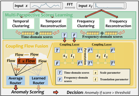
FlowFuse is a multi-view time series anomaly detection framework comprising three core stages:
- Multi-Perspective Scores Learning: The input time series is processed simultaneously in temporal and frequency domains through FFT transformation. Four parallel detectors (Temporal Clustering, Temporal Reconstruction, Frequency Clustering, and Frequency Reconstruction) extract complementary anomaly scores, yielding temporal scores T and frequency scores F.
- Coupling Flow Fusion: An ensemble of E coupling flows models the joint distribution of multi-view scores. Each coupling flow learns complex dependencies between temporal and frequency scores through alternating coupling layers with scale and translation transformations.
- Anomaly Scoring: In unsupervised settings, an average router performs ensemble averaging across all flows. When labeled data is available, a learned router adaptively weights ensemble members based on score uncertainty. The final anomaly decision is made by comparing scores against a threshold.
Figure 1 illustrates the overall architecture. The framework first extracts anomaly scores from four complementary perspectives-clustering and reconstruction methods in both temporal and frequency domains-to capture diverse anomaly characteristics. These multi-view scores are then processed by an ensemble of coupling flows that learn their joint distribution through invertible transformations, producing fused anomaly scores.
The key advantage of using multiple flows is that their score disagreement (variance) naturally quantifies detection uncertainty. High disagreement indicates samples near decision boundaries where the model has low confidence. This uncertainty measure serves dual purposes: it identifies the most informative samples for selective supervision, and it provides practitioners with confidence estimates for detection results. The design ensures the framework operates effectively in purely unsupervised settings while seamlessly incorporating supervision when available to enhance detection performance.
3.3 Multi-Perspective Scores Learning
The framework begins with standardization to ensure comparability across dimensions, followed by adaptive windowing that segments data using a sliding window approach with window length W and stride s, producing overlapping windows Wi ∈ RW×d . The window size W can be automatically determined through FFT-based periodicity detection to align with natural data cycles, or set manually based on domain knowledge. Each window is also transformed via FFT to obtain its frequency representation for parallel processing in both temporal and frequency domains. By default, we set W = 50 and s = 1 across all experiments.
The choice of four detection perspectives is guided by two orthogonal design dimensions:
Domain Dimension (Temporal vs. Frequency). Different anomaly types manifest distinctively across domains. Point anomalies and local contextual anomalies are more apparent in the temporal domain, while seasonal anomalies and harmonic distortions are more naturally captured in the frequency domain.
Paradigm Dimension (Clustering vs. Reconstruction). Clustering-based methods excel at detecting global outliers and novel patterns far from learned clusters. Reconstructionbased methods excel at detecting subtle local deviations through high reconstruction errors.
For each window, we compute anomaly scores from four complementary perspectives:
- Temporal Clustering: We apply K-means clustering to identify C = 24 typical temporal patterns (see Section 4.4) in the training data [Yairi et al., 2001; He et al., 2003]. For each test window, we compute its Euclidean distance to the nearest cluster center. Windows that fall far from all learned clusters likely represent anomalous patterns not seen during training.
- Temporal Reconstruction: We employ a Transformer model with inverted tokenization [Liu et al., 2024; Nie et al., 2023], where each variable's time series serves as a token rather than each time point. The model learns to reconstruct normal temporal patterns through self-attention mechanisms [Xu et al., 2021]. High reconstruction errors indicate deviations from learned normal dependencies.
- Frequency Clustering: After applying FFT to convert windows to the frequency domain, we perform K-means clustering on the magnitude spectra with the same number of clusters C. This captures typical frequency patterns and identifies anomalies with unusual spectral characteristics that temporal analysis might miss [Ren et al., 2019].
- Frequency Reconstruction: A specialized Transformer operates directly on frequency representations (both mag-
nitude and phase), learning to reconstruct normal spectral patterns. This method excels at detecting subtle frequency anomalies like broken periodicities, harmonic distortions, or abnormal frequency components [Thill et al., 2017; Nam et al., 2024; Wu et al., 2024].
Using the same number of clusters C across both temporal and frequency domains ensures balanced representational capacity and consistent granularity, enabling fair integration of clustering-based scores from different perspectives. This multi-view approach leverages the observation that different anomaly types manifest distinctively across domains and detection paradigms. Point anomalies typically show high reconstruction errors, while pattern anomalies are better captured by clustering distances [Liu et al., 2008].
Since we use overlapping sliding windows with stride s, each timestamp may appear in multiple windows. We aggregate these window-level scores to point-level through averaging:
where Wt denotes all windows containing timestamp t [Yeh et al., 2016; Tatbul et al., 2018], and v ∈ {1, 2, 3, 4} indexes the four views. The resulting score matrix St ∈ Rd×4 for each timestamp provides a comprehensive characterization of potential anomalies from multiple perspectives, where each row corresponds to one dimension and each column represents one of the four detection views.
Given the score matrix St ∈ Rd×4 , we partition it along the column dimension into:
- Temporal scores: Tt = St[:, 1:2] ∈ Rd×2 (clustering + reconstruction)
- Frequency scores: Ft = St[:, 3:4] ∈ Rd×2 (clustering + reconstruction)
3.4 Coupling Flow Fusion
Traditional score aggregation methods fail to capture the complex dependencies between different detection methods. Table 1 summarizes the limitations of common approaches.
| Method | Non-linear Modeling | Cross-view Interaction | Distribution Learning |
|---|---|---|---|
| Average | ✗ | ✗ | ✗ |
| Maximum | ✗ | ✗ | ✗ |
| Learned Weights | ✗ | ✗ | ✗ |
| MLP Fusion | ✓ | ✓ | ✗ |
| Coupling Flow (Ours) | ✓ | ✓ | ✓ |
Linear methods (averaging, maximum, learned weights) treat views independently, ignoring their correlations. While MLP-based fusion can model non-linear interactions, it lacks principled density estimation and cannot determine whether a score pattern is normal or anomalous based on the learned distribution. Consider two scenarios: (1) A sample with high temporal but low frequency scores might indicate a temporal anomaly that frequency methods correctly ignore, and averaging dilutes this signal. (2) Moderate scores across all views might indicate a true anomaly through consistent deviation; maximum selection misses this pattern.
Coupling flows address these limitations by modeling the joint distribution p(S) of multi-view scores through invertible transformations with tractable likelihood computation. Samples with low likelihood under the learned normal distribution are identified as anomalies. Since the entire process operates without anomaly labels, this approach performs unsupervised modeling of the complete joint distribution.
Before fusion, all scores are standardized within each variable to zero mean and unit variance, ensuring comparability across different detection methods. Each coupling flow fe : Rd×4 → Rd×4 consists of Lc coupling layers that progressively transform the complex score distribution to a standard Gaussian distribution in latent space.
Coupling Layer Architecture. Each coupling layer applies conditional affine transformations through an alternating scheme. Given the temporal and frequency partitions [T(ℓ) t ,F(ℓ) t ] at layer ℓ, a single coupling block performs:
Step 1: Update frequency scores conditioned on temporal scores:
where sθ, tθ : Rd×2 → Rd×2 are scale and translation networks parameterized by θ, and ⊙ denotes element-wise multiplication.
Step 2: Update temporal scores conditioned on updated frequency scores:
where sϕ, tϕ : Rd×2 → Rd×2 are parameterized by ϕ.
This alternating structure enables bidirectional modeling of dependencies between temporal and frequency domains. The key insight is that by using the updated values from the previous half-step (e.g., F(ℓ+ 12 ) t instead of F(ℓ) t ), the flow can learn complex interactions-how temporal scores relate to frequency scores that have already been contextualized by temporal information.
The complete coupling flow consists of Lc such blocks stacked sequentially:
where zt ∈ Rd×4 is the latent representation. Each layer progressively refines the representation, with later layers capturing higher-order dependencies between views.
Ensemble Strategy. We train an ensemble of E coupling flows {f1, . . . , fE} with different random initializations and data subsets to create diversity. Each flow independently optimizes the negative log-likelihood of observed score patterns:
where z(e) t = fe(St) is the latent representation, ∥ · ∥F denotes the Frobenius norm, and Jfe is the Jacobian matrix of the flow transformation. The first term encourages latent representations to follow a standard Gaussian distribution, while the Jacobian determinant ensures invertibility.
The ensemble improves robustness through model averaging, provides more accurate density estimation with lower variance, and naturally quantifies detection uncertainty through score disagreement ut = VarEe=1 [re(St)]. High variance indicates samples near decision boundaries where individual flows disagree. We adopt E = 4 and Lc = 2 as default across all experiments.
To obtain interpretable anomaly scores, we convert likelihoods to percentile ranks. During training, we store the likelihood distribution for each flow. At test time, for sample St:
where I[·] is the indicator function and re(St) ∈ [0, 1].
3.5 Anomaly Scoring
The final anomaly score adapts to the availability of supervision through two routing strategies. In the unsupervised setting, we use an average router that performs ensemble averaging:
When labeled data becomes available, FlowFuse can optionally employ a learned router that leverages the ensemble's uncertainty measure. We select the top-K highest-uncertainty samples where K = ⌈ptrain · Ntrain⌉, and train a lightweight routing network gψ : Rd×4 → RE that assigns weights to ensemble members:
The router is trained using ranking loss on anomaly-normal pairs from the high-uncertainty subset:
where ϕ(St) = ∑Ee=1 we(St) · re(St) is the router-weighted score. This focuses limited labels on ambiguous regions where supervision has maximum impact.
The ensemble average ¯ r(St) provides robust anomaly scores by aggregating anomaly scores from diverse coupling flows. The weighted score ϕ(St) adaptively combines ensemble members based on the input score pattern, improving detection in previously ambiguous regions. This design ensures FlowFuse operates effectively across the full spectrum from purely unsupervised to semi-supervised settings.
4 Experiment
4.1 Experimental Settings
Datasets
We evaluate FlowFuse on 18 diverse benchmarks covering 10 univariate and 8 multivariate datasets across multiple domains including spacecraft telemetry, server monitoring, healthcare, movement analysis, and industrial systems. These datasets exhibit varied characteristics in dimensionality (155 channels), sequence lengths (785-1,416,825 points), and anomaly ratios (0.20%-15.57%), ensuring robust validation across different operational contexts. Table 2 summarizes all dataset statistics with original sources.
| Dataset | Domain | Dim | Series | Avg Total Length | Avg Test Length | Avg AR (%) | Train AR (%) |
|---|---|---|---|---|---|---|---|
| GAIA | AIOps | 1 | 184 | 9,777 | 8,799 | 1.26 | 0.19 |
| GHL | Machinery | 1 | 1 | 200,001 | 180,001 | 0.43 | 0.00 |
| KDD21 | Multiple | 1 | 243 | 65,903 | 47,294 | 0.58 | 0.00 |
| MGAB | Synthetic | 1 | 6 | 100,000 | 90,000 | 0.20 | 0.00 |
| NASA-MSL | Spacecraft | 1 | 22 | 5,167 | 2,897 | 3.85 | 0.00 |
| NAB | Multiple | 1 | 45 | 7,115 | 3,557 | 9.84 | 6.55 |
| OPPORTUNITY | Movement | 1 | 462 | 31,359 | 28,223 | 4.12 | 19.11 |
| NASA-SMAP | Spacecraft | 1 | 35 | 10,539 | 7,930 | 2.20 | 0.00 |
| SVDB | Health | 1 | 52 | 230,400 | 207,360 | 4.87 | 5.48 |
| YAHOO | Multiple | 1 | 346 | 1,570 | 785 | 0.63 | 0.46 |
| LTDB | Health | 2 | 5 | 100,000 | 87,285 | 15.57 | 11.72 |
| MITDB | Health | 2 | 6 | 141,667 | 106,250 | 2.72 | 0.00 |
| MSL | Spacecraft | 55 | 1 | 132,046 | 73,729 | 5.88 | 0.00 |
| SMD | Server | 38 | 1 | 1,416,825 | 708,420 | 2.08 | 0.00 |
| NYC | Transport | 3 | 1 | 17,520 | 4,416 | 0.57 | 0.00 |
| PSM | Server | 25 | 1 | 220,322 | 87,841 | 11.07 | 0.00 |
| SMAP | Spacecraft | 25 | 1 | 562,800 | 427,617 | 9.72 | 0.00 |
| SVDB | Health | 2 | 6 | 110,133 | 86,373 | 3.14 | 5.48 |
Dataset types distinguished by row color: Cyan = 10 Univariate (GAIA-YAHOO); Yellow = 8 Multivariate (LTDB-SVDB).
Table 2: Summary of evaluation datasets. AR denotes anomaly ratio.
Baselines
We compare against 18 state-of-the-art methods spanning three major anomaly detection paradigms: statistical distribution-based approaches (6 methods), reconstructionbased methods (10 methods), and discriminative learning approaches (2 methods), as detailed in Table 4. The baselines encompass non-learning statistical methods, traditional machine learning algorithms, and modern deep learning architectures.
Setup
We utilize TAB [Qiu et al., 2025a] for unified evaluation, with all baseline results derived from the same framework. To ensure fair comparison and demonstrate robustness, we employ a single set of hyperparameters for all univariate datasets and another for all multivariate datasets, without dataset-specific tuning. We adopt two evaluation metrics: Affiliated F1score [Huet et al., 2022] for label-based evaluation and AUROC for score-based evaluation. Hyperparameter configurations are detailed in Section 4.4.
4.2 Main Results
Table 3 presents evaluation results on both univariate and multivariate datasets, distinguished by background color (cyan for univariate, yellow for multivariate). FlowFuse achieves the best performance on the majority of benchmarks, demonstrating strong generalization across diverse anomaly detection scenarios.
For univariate time series, FlowFuse obtains impressive results on challenging datasets with complex temporal patterns (e.g., GHL, SMAP, YAHOO), while maintaining consistent superiority in ranking quality as measured by AUC-ROC. On multivariate benchmarks, our method delivers robust performance by effectively capturing cross-dimensional dependen-
| Dataset | Metric | Ours | Modern | DualTF | iTrans | ATrans | DC | TranAD | ConAD | Patch | DLin | VAE | DAGMM | KNN | KMeans | OCSVM | IF | DP | LOF | |
|---|---|---|---|---|---|---|---|---|---|---|---|---|---|---|---|---|---|---|---|---|
| GAIA GHL MGAB | Aff-F A-R Aff-F | 0.871 0.872 0.975 0.998 0.895 0.887 0.793 | 0.904 0.821 0.723 0.493 0.718 0.534 0.678 0.561 0.896 | 0.753 0.564 0.682 0.374 0.698 0.569 0.675 0.576 0.766 0.537 0.782 0.550 0.710 | 0.907 0.823 0.709 0.498 0.767 0.605 0.691 0.501 0.865 0.724 0.832 | 0.697 0.446 0.652 0.476 0.698 0.499 0.671 0.500 0.743 | 0.711 0.411 0.669 0.498 0.686 0.493 | 0.790 0.756 0.577 0.020 0.723 0.528 0.670 0.592 0.902 | 0.683 0.486 0.667 0.500 0.685 0.502 0.667 0.522 0.673 0.500 0.701 | 0.902 0.819 0.735 0.500 | 0.897 0.801 0.730 | 0.727 0.748 | 0.598 0.648 0.465 0.020 | 0.759 0.821 0.679 0.751 0.678 0.638 0.666 0.560 | 0.781 0.738 0.598 0.747 0.822 0.778 0.688 | 0.725 0.726 0.667 0.751 0.669 0.590 | 0.731 0.695 0.687 0.500 0.675 0.554 0.664 | 0.673 0.755 0.667 0.888 0.667 0.532 0.667 0.515 0.673 | 0.737 0.817 0.679 0.751 0.675 0.584 0.667 0.509 0.772 | HBOS 0.689 0.687 0.638 0.662 0.666 0.564 0.665 |
| A-R | 0.751 | 0.616 0.858 | 0.528 | 0.555 0.087 | ||||||||||||||||
| KDD21 | Aff-F A-R | 0.713 0.529 | 0.726 0.538 | 0.652 0.540 | 0.640 0.538 | |||||||||||||||
| Aff-F A-R | 0.773 | 0.673 0.504 | 0.669 0.559 | 0.668 0.567 | 0.664 0.555 | 0.620 0.545 | 0.605 | 0.666 0.550 | 0.487 | 0.586 | ||||||||||
| MSL | Aff-F A-R | 0.922 0.803 0.828 | 0.726 0.838 | 0.426 | 0.757 0.469 | 0.883 0.727 | 0.903 0.710 | 0.686 0.652 | 0.609 0.609 | 0.775 0.673 | 0.894 0.725 | 0.795 0.666 | 0.658 0.561 | 0.636 0.680 | 0.614 | 0.733 0.607 | ||||
| NAB | Aff-F A-R | 0.640 0.788 | 0.612 0.733 | 0.411 | 0.614 0.709 | 0.469 0.728 | 0.714 0.506 | 0.546 | 0.506 0.770 | 0.848 0.605 | 0.850 0.608 | 0.739 0.556 | 0.620 0.572 0.628 | 0.730 0.563 0.656 | 0.818 0.626 0.734 | 0.722 0.584 | 0.711 0.535 | 0.531 0.667 | 0.695 0.545 | 0.744 0.570 |
| OPP | Aff-F A-R Aff-F | 0.664 0.967 | 0.215 0.913 | 0.686 | 0.224 0.928 | 0.665 0.764 0.480 | 0.679 0.503 0.760 | 0.762 0.559 0.851 | 0.504 0.680 | 0.732 0.217 0.906 | 0.737 0.304 | 0.674 0.514 0.595 | 0.578 0.569 | 0.461 0.717 | 0.285 0.886 | 0.654 0.487 0.698 | 0.654 0.242 | 0.260 0.674 | 0.671 0.545 0.711 | 0.653 0.522 |
| SMAP SVDB | A-R Aff-F A-R | 0.899 0.833 0.780 | 0.694 0.733 0.573 | 0.535 0.745 0.586 | 0.752 0.718 0.576 | 0.686 0.504 0.671 | 0.487 0.685 0.460 | 0.520 0.730 0.549 | 0.502 0.682 0.500 | 0.707 0.727 0.569 | 0.906 0.615 0.728 | 0.596 0.683 | 0.586 0.611 | 0.594 0.710 | 0.802 0.735 | 0.586 0.698 0.567 | 0.655 0.513 0.672 0.544 | 0.655 0.682 0.531 | 0.551 0.709 0.516 | 0.647 0.526 0.700 |
| YAHOO | Aff-F A-R | 0.914 0.936 | 0.793 0.804 | 0.748 0.467 | 0.897 0.891 | 0.477 | 0.629 0.490 | 0.755 0.697 | 0.678 0.488 | 0.800 0.828 | 0.580 0.825 0.843 | 0.570 0.615 0.756 | 0.549 0.453 0.707 | 0.520 0.661 0.734 | 0.683 0.604 0.589 | 0.675 0.639 | 0.897 0.924 | 0.669 0.862 | 0.664 0.754 | 0.553 0.653 0.678 |
| LTDB | Aff-F A-R | 0.794 0.833 0.925 | 0.777 0.619 0.803 | 0.455 0.589 | 0.756 0.579 | 0.702 0.505 0.700 0.424 | 0.710 0.494 0.689 | 0.790 0.590 | 0.752 0.576 0.694 | 0.767 0.587 0.813 | 0.764 0.599 0.722 | 0.670 0.610 0.713 | 0.653 0.545 0.689 | 0.768 0.632 | 0.724 0.738 | 0.754 0.615 | 0.644 0.559 | 0.724 0.551 | 0.763 0.621 0.700 | 0.759 0.611 |
| MITDB | Aff-F A-R Aff-F | 0.767 0.738 0.645 0.794 | 0.663 0.726 0.621 | 0.843 0.693 0.258 0.499 | 0.806 0.679 0.705 0.589 | 0.685 0.502 | 0.503 0.674 0.500 | 0.848 0.691 0.724 0.478 | 0.488 0.671 0.548 | 0.676 0.714 0.621 | 0.583 0.723 0.601 | 0.667 0.642 0.530 | 0.682 0.723 0.569 | 0.709 0.692 0.696 | 0.834 0.692 0.580 | 0.700 0.689 0.641 | 0.709 0.618 0.584 0.524 | 0.678 0.598 0.677 0.488 | 0.627 0.701 0.557 | 0.687 0.681 0.680 |
| MSL SMD | A-R Aff-F A-R | 0.749 0.946 0.808 | 0.839 0.721 0.693 | 0.679 0.703 0.676 | 0.817 0.745 0.683 0.594 | 0.674 0.509 0.732 0.859 | 0.674 0.500 0.674 0.526 | 0.789 0.663 | 0.023 0.491 0.714 0.443 | 0.830 0.736 0.805 0.667 | 0.834 0.708 0.725 0.699 | 0.450 0.641 0.767 0.661 | 0.023 0.527 0.694 | 0.623 0.696 0.716 0.644 | 0.603 0.686 0.713 | 0.524 0.742 0.602 0.667 0.456 | 0.626 0.664 0.648 0.475 | 0.674 0.672 0.668 | 0.682 0.645 0.652 0.464 | 0.574 0.629 0.626 0.675 |
| NYC PSM | Aff-F A-R Aff-F A-R | 0.739 0.635 0.551 | 0.696 0.823 0.587 | 0.723 0.725 0.544 | 0.855 0.583 0.746 0.636 | 0.634 0.499 0.501 | 0.671 0.499 0.681 0.500 | 0.796 0.676 0.748 0.635 | 0.648 0.533 0.430 0.364 | 0.836 0.583 0.441 0.787 | 0.832 0.559 0.391 0.727 | 0.295 0.642 0.697 | 0.573 0.463 0.637 | 0.466 0.695 0.744 | 0.646 0.833 0.735 0.732 | 0.531 0.619 0.503 | 0.620 0.542 | 0.476 0.694 0.539 | 0.694 0.730 | 0.446 0.658 0.714 |
| SMAP | Aff-F A-R | 0.468 | 0.616 0.434 | 0.674 0.465 | 0.577 0.409 | 0.692 | 0.538 0.369 | 0.694 | 0.629 | 0.607 | 0.487 0.412 | 0.430 0.573 | 0.630 0.629 | 0.517 0.405 | 0.393 | 0.512 0.487 | 0.681 0.429 | 0.642 0.626 | 0.509 0.585 | |
| SVDB | Aff-F A-R | 0.896 0.913 | 0.746 | 0.585 0.555 | 0.752 | 0.533 | 0.692 | 0.733 | 0.820 | 0.723 | 0.708 | 0.734 | 0.735 0.568 | |||||||
| 0.593 | 0.595 | 0.585 | 0.692 0.527 | 0.580 | ||||||||||||||||
| 0.701 0.491 | 0.711 0.464 | 0.577 | 0.651 | 0.610 | 0.570 | 0.564 | 0.839 | 0.533 |
Dataset types distinguished by row color: Cyan = 10 Univariate (GAIA-YAHOO); Yellow = 8 Multivariate (LTDB-SVDB).
| Paradigm | Method | Abbrev. |
|---|---|---|
| Statistical Distribution-based | • LOF [Breunig et al., 2000] • KNN • Isolation Forest [Liu et al., 2008] • HBOS [Goldstein and Dengel, 2012] • OC-SVM [Sch¨olkopf et al., 1999] • K-Means [Yairi et al., 2001] | LOF KNN IF HBOS OCSVM KMeans |
| Reconstruction-based | • VAE [Kingma and Welling, 2013] • DAGMM [Zong et al., 2018] • DeepPoint [Bhatnagar et al., 2021] • TranAD [Tuli et al., 2022] • Anomaly Transformer [Xu et al., 2021] • DualTF [Nam et al., 2024] • PatchTST [Nie et al., 2023] •ModernTCN [Luo andWang, 2024] • DLinear [Zeng et al., 2023] • iTransformer [Liu et al., 2024] | VAE DAGMM DP TranAD ATrans DualTF Patch Modern DLin iTrans |
| Discriminative Learning | • DCdetector [Yang et al., 2023b] • ContraAD [Zhuang et al., 2025] | DC ConAD |
| Variations | LTDB | MSL | SMAP | SVDB | Avg. | |
|---|---|---|---|---|---|---|
| Simple Averaging | 0.745 | 0.683 | 0.433 | 0.798 | 0.665 | |
| Multi- w/o Temporal Clustering | 0.721 | 0.652 | 0.412 | 0.785 | 0.643 | |
| View w/o Temporal Reconstruction | 0.726 | 0.715 | 0.368 | 0.800 | 0.652 | |
| Scores w/o Frequency Clustering | 0.755 | 0.698 | 0.527 | 0.801 | 0.695 | |
| w/o Frequency Reconstruction | 0.768 | 0.710 | 0.522 | 0.785 | 0.696 | |
| FlowFuse (Full) | 0.794 | 0.738 | 0.551 | 0.896 | 0.745 | |
Table 5: Ablation studies for FlowFuse in terms of Aff-F1.
cies through the coupling flow mechanism, achieving top results on LTDB, MITDB, NYC, and SVDB.
Compared to recent deep learning methods such as ModernTCN, DualTF, and Anomaly Transformer, FlowFuse demonstrates more stable performance across different data characteristics. While these baseline methods often excel on specific datasets but struggle on others, our approach maintains competitive results throughout all 18 benchmarks, validating the effectiveness of multi-view ensemble fusion.
4.3 Ablation Studies
To validate the contribution of each component in FlowFuse, we conduct comprehensive ablation studies on four representative datasets. Table 5 presents the results.
The results demonstrate that: (1) coupling flow fusion significantly outperforms simple averaging (+8.0% on average), validating the importance of modeling non-linear score dependencies; (2) each multi-view component contributes to overall performance, with temporal views showing larger impact than frequency views on most datasets; (3) the full model achieves the best results, confirming the complementary nature of all four detection perspectives.
4.4 Further Analysis
Method-Specific Detection Bias
To illustrate multi-view fusion rationale, we analyze 35 methods spanning three detection paradigms (listed in our repository) on datasets grouped by anomaly types. Figure 2 presents VUS-PR performance distributions across six anomaly categories, each subfigure visualizing method performance variation for a specific type.
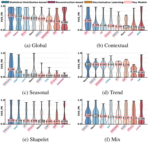
Notably, we observe distinct paradigm tendencies: deep learning methods (e.g., iTransformer [Liu et al., 2024], DLinear [Zeng et al., 2023]) work effectively for point anomalies (global, contextual; Figure 2(a)(b)), while statistical approaches (e.g., KMeans, DWT [Thill et al., 2017], HBOS) are more suitable for subsequence anomalies (seasonal, shapelet; Figure 2(c)(e)). Additionally, even top-performing methods achieve only moderate performance on mixed anomalies (Figure 2(f)), lower than their performance on single-type anomalies.
This observation supports FlowFuse's multi-view fusion design. Integrating complementary perspectives via coupling flows, FlowFuse maintains stable performance across all six categories, alleviating constraints of type-specialized detection methods. The complete list of 35 methods and their implementations is available in our repository.
Optional Supervised Enhancement
When labeled data is available, FlowFuse can optionally refine detection through uncertainty-guided supervision. Table 6 shows performance with varying label ratios.
The results reveal that: (1) unsupervised FlowFuse already achieves strong baseline performance; (2) small amounts of labeled data (1-5%) yield substantial improvements, with diminishing returns at higher ratios; (3) performance saturates quickly, validating the uncertainty-guided sample selection strategy that focuses supervision on the most informative samples.
| Dataset | Unsup. (0%) | Label Ratio (%) | ||||
|---|---|---|---|---|---|---|
| 1 | 5 | 20 | 50 | 100 | ||
| NAB | 0.640 | 0.680 | 0.700 | 0.710 | 0.700 | 0.703 |
| SVDB | 0.780 | 0.810 | 0.820 | 0.820 | 0.820 | 0.820 |
| YAHOO | 0.936 | 0.941 | 0.945 | 0.944 | 0.945 | 0.945 |
| LTDB | 0.833 | 0.847 | 0.853 | 0.858 | 0.860 | 0.857 |
Parameter Sensitivity
We investigate the sensitivity of FlowFuse to two key hyperparameters: the number of clusters C and the number of coupling flows E. Figure 3 presents the results on four benchmark datasets.
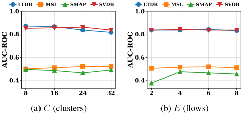
For the number of clusters C, FlowFuse maintains stable performance across the range of 8 to 32, with less than 3% variation for most datasets. For the number of flows E, performance improves from E = 2 to E = 4 then saturates, indicating diminishing returns from additional ensemble members. We adopt E = 4 as the default. Overall, FlowFuse exhibits robust performance across its hyperparameter space without requiring precise tuning.
5 Conclusion
In this paper, we proposed FlowFuse, a multi-view ensemble framework that addresses anomaly diversity through coupling flow-based score fusion. By modeling the joint distribution of four complementary detection perspectives spanning temporal and frequency domains, as well as clustering and reconstruction paradigms, FlowFuse captures complex inter-view dependencies that linear aggregation cannot express. An ensemble of coupling flows provides robustness and natural uncertainty quantification, which enables targeted supervision when labels are available. Experiments on 18 benchmarks demonstrate state-of-the-art performance across diverse anomaly types, validating that principled multi-view fusion enables more comprehensive anomaly detection.
Ethical Statement
Our work uses only publicly available benchmark datasets without personally identifiable information. The proposed anomaly detection framework is for beneficial system reliability and safety monitoring applications, and no human subjects were involved in this research.
Acknowledgments
This work was partially supported by the National Natural Science Foundation of China (62372179) and the InnoHK funding.
Contribution Statement
Wanghui Qiu and Chenxi Liu contributed equally to this work as co-first authors. Bin Yang is the corresponding author.
@inproceedings{ijcai2026p332,
  title     = {Multi-View Ensemble for Time Series Anomaly Detection via Coupling Flows},
  author    = {Qiu, Wanghui and Liu, Chenxi and Hu, Shiyan and Li, Zhengyu and Guo, Chenjuan and Yang, Bin},
  booktitle = {Proceedings of the Thirty-Fifth International Joint Conference on
               Artificial Intelligence, {IJCAI-26}},
  publisher = {International Joint Conferences on Artificial Intelligence Organization},
  editor    = {Diego Calvanese},
  pages     = {2988--2996},
  year      = {2026},
  month     = {8},
  note      = {Main Track},
  doi       = {10.24963/ijcai.2026/332},
  url       = {https://doi.org/10.24963/ijcai.2026/332},
}
TY - CPAPER TI - Multi-View Ensemble for Time Series Anomaly Detection via Coupling Flows AU - Qiu, Wanghui AU - Liu, Chenxi AU - Hu, Shiyan AU - Li, Zhengyu AU - Guo, Chenjuan AU - Yang, Bin T2 - Proceedings of the Thirty-Fifth International Joint Conference on Artificial Intelligence, IJCAI-26 PB - International Joint Conferences on Artificial Intelligence Organization PY - 2026 SP - 2988 EP - 2996 DO - 10.24963/ijcai.2026/332 UR - https://doi.org/10.24963/ijcai.2026/332 ER -Copied
Machine-readable versions of this paper, for tools and AI agents:





