
Do Not Discretize, Optimize: Almost Greedy Fictitious Play
Proceedings of the Thirty-Fifth International Joint Conference on Artificial Intelligence. Main Track. Pages 3505-3513.
https://doi.org/10.24963/ijcai.2026/390
Keywords
- Machine Learning: Game Theory
- Game Theory and Economic Paradigms: Noncooperative games
Abstract
Our work evolves around Fictitious Play, one of the first iterative methods that is known to converge to a Nash equilibrium in zero-sum games. In recent years, there has been a revived interest, due to applications in various machine learning problems, which has motivated a line of work on its convergence properties and on proposing new variants of the initial algorithm. Our paper is along this direction and introduces one new variant, which we refer to as Almost Greedy Fictitious Play. The proposed algorithm greedily attempts to find the optimal stepsize at each iteration but its search space is constrained and includes almost all the line between the cumulative mixed strategy and the current best response. Our main result is that the method achieves an instance dependent convergence rate of O(1/T) with respect to the duality gap. This matches the rate of Continuous Fictitious Play, and offers an alternative to discretization. We complement our theoretical findings with experiments that demonstrate the effectiveness of the method.
- [Abernethy et al., 2021] Jacob Abernethy, Kevin A Lai, and Andre Wibisono. Fast convergence of fictitious play for di- agonal payoff matrices. In Proceedings of the 2021 ACM- SIAM Symposium on Discrete Algorithms (SODA), pages 1387-1404. SIAM, 2021.
- [Anagnostides and Sandholm, 2024] Ioannis Anag- nostides and Tuomas Sandholm. Convergence of $\text{log}(1/\epsilon)$ for gradient-based algorithms in zero-sum games without the condition number: A smoothed analysis. In Advances in Neural Information Processing Systems 38: Annual Conference on Neural Information Processing Systems 2024, NeurIPS 2024, Vancouver, BC, Canada, December 10 -15, 2024, 2024.
- [Baudin and Laraki, 2022a] Lucas Baudin and Rida Laraki. Fictitious play and best-response dynamics in identical in- terest and zero-sum stochastic games. In International Conference on Machine Learning, ICML 2022, 17-23 July 2022, Baltimore, Maryland, USA, volume 162 of Proceed- ings of Machine Learning Research, pages 1664-1690. PMLR, 2022.
- [Baudin and Laraki, 2022b] Lucas Baudin and Rida Laraki. Smooth fictitious play in stochastic games with perturbed payoffs and unknown transitions. In Advances in Neural Information Processing Systems 35: Annual Conference on Neural Information Processing Systems 2022, NeurIPS 2022, New Orleans, LA, USA, November 28 -December 9, 2022, 2022.
- [Brandt et al., 2010] Felix Brandt, Felix Fischer, and Paul Harrenstein. On the rate of convergence of fictitious play. In International Symposium on Algorithmic Game Theory, pages 102-113. Springer, 2010.
- [Brown, 1949] George W Brown. Some notes on computa- tion of games solutions. Technical report, The Rand Cor- poration, 1949.
- [Brown, 1951] George W Brown. Iterative solution of games by fictitious play. Act. Anal. Prod Allocation, 13(1):374, 1951.
- [Chen et al., 2022] Yurong Chen, Xiaotie Deng, Chenchen Li, David Mguni, Jun Wang, Xiang Yan, and Yaodong Yang. On the convergence of fictitious play: A decompo- sition approach. In Proceedings of the Thirty-First Inter- national Joint Conference on Artificial Intelligence, IJCAI 2022, Vienna, Austria, 23-29 July 2022, pages 179-185. IJCAI
- [Cloud et al., 2023] Alex Cloud, Albert Wang, and Wesley Kerr. Anticipatory fictitious play. In Proceedings of the Thirty-Second International Joint Conference on Artificial Intelligence, IJCAI 2023, 19th-25th August 2023, Macao, SAR, China, pages 73-81. ijcai.org, 2023. IJCAI
- [Daskalakis and Pan, 2014] Constantinos Daskalakis and Qinxuan Pan. A counter-example to karlin's strong conjecture for fictitious play. In 2014 IEEE 55th Annual Symposium on Foundations of Computer Science, pages 11-20. IEEE, 2014.
- [Fasoulakis et al., 2025] Michail Fasoulakis, Evangelos Markakis, Georgios Roussakis, and Christodoulos San- torinaios. A descent-based method on the duality gap for solving zero-sum games. In Proceedings of the Thirty-Fourth International Joint Conference on Artificial Intelligence, IJCAI 2025, Montreal, Canada, August 16-22, 2025, pages 3839-3847. ijcai.org, 2025.
- [Frank and Wolfe, 1956] Marguerite Frank and Philip Wolfe. An algorithm for quadratic programming. Naval research logistics quarterly, 3(1-2):95-110, 1956.
- [Fudenberg and Kreps, 1993] Drew Fudenberg and David M Kreps. Learning mixed equilibria. Games and economic behavior, 5(3):320-367, 1993.
- [Fudenberg and Levine, 1995] Drew Fudenberg and David K Levine. Consistency and cautious fictitious play. Journal of Economic Dynamics and Control, 19(5-7):1065-1089, 1995.
- [Gidel et al., 2017] Gauthier Gidel, Tony Jebara, and Simon Lacoste-Julien. Frank-wolfe algorithms for saddle point problems. In Proceedings of the 20th International Con- ference on Artificial Intelligence and Statistics, AISTATS 2017, 20-22 April 2017, Fort Lauderdale, FL, USA, vol- ume 54 of Proceedings of Machine Learning Research, pages 362-371. PMLR, 2017.
- [Goldman and Tucker, 1956] Alan J Goldman and Albert W Tucker. Theory of linear programming. Linear inequalities and related systems, 38:53-97, 1956.
- [Goodfellow et al., 2014] Ian J. Goodfellow, Jean Pouget- Abadie, Mehdi Mirza, Bing Xu, David Warde-Farley, Sherjil Ozair, Aaron C. Courville, and Yoshua Bengio. Generative adversarial nets. In Advances in Neural In- formation Processing Systems 27: Annual Conference on Neural Information Processing Systems 2014, December 8-13 2014, Montreal, Quebec, Canada, pages 2672-2680, 2014.
- [Harris, 1998] Christopher Harris. On the rate of conver- gence of continuous-time fictitious play. Games and Eco- nomic Behavior, 22(2):238-259, 1998.
- [Heinrich et al., 2015] Johannes Heinrich, Marc Lanctot, and David Silver. Fictitious self-play in extensive-form games. In International conference on machine learning, pages 805-813. PMLR, 2015.
- [Hofbauer and Sandholm, 2002] Josef Hofbauer and William H Sandholm. On the global convergence of stochastic fictitious play. Econometrica, 70(6):2265- 2294, 2002.
- [Karlin, 1959] Samuel Karlin. Mathematical methods and theory in games, programming and economics. Addison- Wesley, Reading, 1959.
- [Krishna and Sjöström, 1997] Vijay Krishna and Tomas Sjöström. Learning in games: Fictitious play dynamics. In Cooperation: Game-Theoretic Approaches, pages 257- 273. Springer, 1997.
- [Lazarsfeld et al., 2025a] John Lazarsfeld, Georgios Pil- iouras, Ryann Sim, and Stratis Skoulakis. Optimism with- out regularization: Constant regret in zero-sum games. In Advances in Neural Information Processing Systems 38 (NeurIPS 2025), volume 38, San Diego, CA, USA, 2025.
- [Lazarsfeld et al., 2025b] John Lazarsfeld, Georgios Pil- iouras, Ryann Sim, and Andre Wibisono. Fast and furious symmetric learning in zero-sum games: Gradient descent as fictitious play. In The Thirty Eighth Annual Conference on Learning Theory, 30-4 July 2025, Lyon, France, vol- ume 291 of Proceedings of Machine Learning Research, pages 3527-3577. PMLR, 2025.
- [Ma et al., 2017] Wei-Chiu Ma, De-An Huang, Namhoon Lee, and Kris M Kitani. Forecasting interactive dynamics of pedestrians with fictitious play. In Proceedings of the IEEE Conference on Computer Vision and Pattern Recog- nition, pages 774-782, 2017.
- [Marden et al., 2009] Jason R Marden, Gürdal Arslan, and Jeff S Shamma. Joint strategy fictitious play with iner- tia for potential games. IEEE Transactions on Automatic Control, 54(2):208-220, 2009.
- [Miyasawa, 1961] Koichi Miyasawa. On the convergence of the learning process in a 2 x 2 non-zero-sum two-person game. Research Memorandum 33, Economic Research Program, Princeton University, 1961.
- [Monderer and Sela, 1996] Dov Monderer and Aner Sela. A 2×2 game without the fictitious play property. Games and Economic Behavior, 14(1):144-148, 1996.
- [Monderer and Shapley, 1996a] Dov Monderer and Lloyd S Shapley. Fictitious play property for games with identi- cal interests. Journal of economic theory, 68(1):258-265, 1996.
- [Monderer and Shapley, 1996b] Dov Monderer and Lloyd S Shapley. Potential games. Games and economic behavior, 14(1):124-143, 1996.
- [Muller et al., 2020] Paul Muller, Shayegan Omidshafiei, Mark Rowland, Karl Tuyls, Julien Pérolat, Siqi Liu, Daniel Hennes, Luke Marris, Marc Lanctot, Edward Hughes, Zhe Wang, Guy Lever, Nicolas Heess, Thore Graepel, and Rémi Munos. A generalized training approach for multia- gent learning. In 8th International Conference on Learn- ing Representations, ICLR 2020, Addis Ababa, Ethiopia, April 26-30, 2020. OpenReview.net, 2020.
- [Nash, 1951] John Nash. Non-cooperative games. Annals of Mathematics, 54(2):286-295, 1951.
- [Ostrovski and van Strien, 2013] Georg Ostrovski and Se- bastian van Strien. Payoff performance of fictitious play. CoRR, abs/1308.4049, 2013.
- [Panageas et al., 2023] Ioannis Panageas, Nikolas Patris, Stratis Skoulakis, and Volkan Cevher. Exponential lower bounds for fictitious play in potential games. In Ad- vances in Neural Information Processing Systems 36: An- nual Conference on Neural Information Processing Sys- tems 2023, NeurIPS 2023, New Orleans, LA, USA, De- cember 10 -16, 2023, 2023.
- [Robinson, 1951] Julia Robinson. An iterative method of solving a game. Annals of mathematics, 54(2):296-301, 1951.
- [Sayin et al., 2022] Muhammed O Sayin, Francesca Parise, and Asuman Ozdaglar. Fictitious play in zero-sum stochastic games. SIAM Journal on Control and Optimiza- tion, 60(4):2095-2114, 2022.
- [Shapley, 1964] Lloyd S Shapley. Some topics in two-person games. Advances in Game Theory.(AM-52), pages 1-28, 1964.
- [Vinyals et al., 2019] Oriol Vinyals, Igor Babuschkin, Woj- ciech M Czarnecki, Michaël Mathieu, Andrew Dudzik, Junyoung Chung, David H Choi, Richard Powell, Timo Ewalds, Petko Georgiev, et al. Grandmaster level in star- craft ii using multi-agent reinforcement learning. Nature, 575(7782):350-354, 2019.
- [von Neumann, 1928] John von Neumann. Zur theorie der gesellschaftsspiele. Mathematische Annalen, 100(1):295- 320, 1928.
- [Wang, 2025] Yuanhao Wang. Tie-breaking agnostic lower bound for fictitious play. arXiv preprint arXiv:2507.09902, 2025.
- [Wei et al., 2021] Chen-Yu Wei, Chung-Wei Lee, Mengxiao Zhang, and Haipeng Luo. Linear last-iterate convergence in constrained saddle-point optimization. In 9th Inter- national Conference on Learning Representations, ICLR 2021, Virtual Event, Austria, May 3-7, 2021. OpenRe- view.net, 2021.
- [Yang and Wang, 2020] Yaodong Yang and Jun Wang. An overview of multi-agent reinforcement learning from game theoretical perspective. arXiv preprint arXiv:2011.00583, 2020.
- [Yang et al., 2018] Yaodong Yang, Rui Luo, Minne Li, Ming Zhou, Weinan Zhang, and Jun Wang. Mean field multi- agent reinforcement learning. In Proceedings of the 35th International Conference on Machine Learning, ICML 2018, Stockholmsmässan, Stockholm, Sweden, July 10-15, 2018, volume 80 of Proceedings of Machine Learning Re- search, pages 5567-5576. PMLR, 2018.
References were extracted automatically from the PDF and may contain errors.
Full text extracted automatically from the PDF; figures, tables and equations may differ. The PDF is the version of record.
1 Introduction
Computing Nash equilibria in two-player bilinear zero-sum games is a cornerstone of Algorithmic Game Theory with a research trajectory spanning several decades. While zerosum games are solvable via linear programming, such centralized approaches often prove computationally prohibitive in large-scale problems. This has led to a resurgence of interest in iterative methods suitable for machine learning applications such as formulating Generative Adversarial Networks (GANs), [Goodfellow et al., 2014]. In this context, the goal is to design simple iterative algorithms that converge efficiently to a Nash equilibrium, where no player has an incentive to deviate.
To this end, we revisit the classic Fictitious Play algorithm, [Brown, 1949]. This is one of the first algorithms ever proposed for zero-sum games, based on a very intuitive idea. At every iteration each player selects a best response to the empirical average of the other player's history. The new strategy profile at each iteration is then updated to the new empirical average, where the probability of each pure strategy equals its selection frequency so far. Alternatively, we can think of the update rule as selecting a particular convex combination between the (mixed) strategy of the previous iteration and the pure best response strategy identified in the current iteration.
Motivated by the latter formulation of Fictitious Play, one can think of defining greedy variants as follows: if at iteration t, we are at the profile (xt, yt) and the best response of the two players are i, j respectively, we could choose in a greedy manner the step size ηt, which is the probability we assign to the best responses, while keeping a probability of 1 - ηt for (xt, yt). One natural metric for making such a choice is the Duality Gap, which represents the sum of regrets of the two players. Therefore, we could pick the stepsize so as to minimize the duality gap over all possible convex combinations, i.e., over ηt ∈ [0, 1]. We refer to this variant as Greedy Fictitious Play.
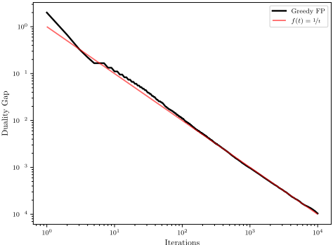
In order to highlight some further intuition on this variant, we illustrate how Greedy Fictitious Play runs for the classic Rock-Paper-Scissors (RPS) game in Figure 1. We also show the stepsizes ηt computed during the first 10 iterations in Table 1. The encouraging news from this illustration is that the duality gap seems to be dropping at a rate of 1/t over time. Let us also take a closer look at the evolution of the step sizes. Under our initialization, both players start by playing Rock. Given this, at iteration 1, the theoretically optimal greedy choice is to set η1 = 2/3. In this case, the next profiles would be 1/3 Rock and 2/3 Paper. Now the best response is not unique: it can be either Paper or Scissors. Assuming we are breaking the ties lexicographically, the best response would again be Paper for each player, resulting in η2 = 0 and the algorithm cannot further progress.
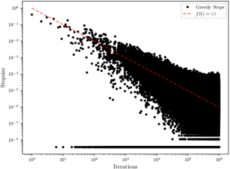
However, due to numerical precision issues, the algorithm selects a slightly larger stepsize which leads to Scissors being selected as a unique best response, instead of Paper. This also occurs in the next few iterations. The next interesting thing to observe is at iteration 5. There, theoretically, the correct step size would have been ηt = 0, and the algorithm would get stuck. But, again due to the numerical precision, the computed step size is slightly positive, and this added noise eventually helps the method to get unstuck. This also occurs in subsequent iterations, as shown in Figure 2, and it motivates the question of whether we could introduce this added noise explicitly in the method.
Iterations
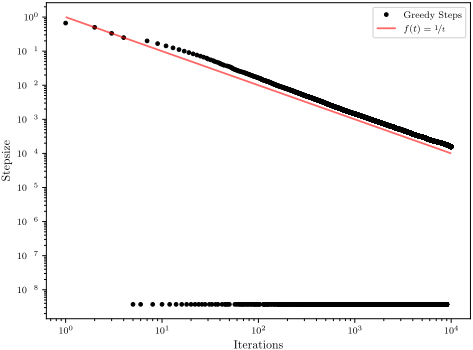
Figure 2: The steps the algorithm selected greedily
1.1 Contributions
Motivated by the previous considerations, we study a slight variation of the algorithm discussed previously, which we term Almost Greedy Fictitious Play (AGFP). The only difference with Greedy Fictitious Play is that we do not optimize the selection of the stepsize ηt over [0, 1], but instead over [δ, 1], for some appropriately selected noise δ.
We study this method both theoretically and experimentally. We first analyze the convergence rate of the method w.r.t. the standard duality gap metric. In particular, for a game with payoff matrix A, we prove that it converges to an approximate Nash equilibrium at a rate of O( 1 κAT ), where κA is a condition-like number, formally defined in Definition 5. Such game-dependent quantities appear often in the convergence analysis of other algorithms (e.g. in the gradient descent family), where the general goal is to move from a O( 1 T ) rate to the improved O(cT ) (see for instance [Wei et al., 2021]). In our case, this constant is necessary even for the sublinear rate.
| t | Greedy stepsize |
| 1 | 0.666666668 |
| 2 | 0.500000004 |
| 3 | 0.333333340 |
| 4 | 0.250000004 |
| 5 | 3.7 × 10⁻⁹ |
| 6 | 3.7 × 10⁻⁹ |
| 7 | 0.200000007 |
| 8 | 3.7 × 10⁻⁹ |
| 9 | 0.166666675 |
| 10 | 3.7 × 10⁻⁹ |
We then turn to an experimental evaluation where our results convey an even better picture. We have tested our method in random games, and we first observe that it is a faster method than the classic FP algorithm. Furthermore, as demonstrated in Section 4, the convergence rate seems to be in the order of O(n/T ), where n is the dimension of the game (replaced by max{n, m} if the payoff matrix is m×n). This matches the rate of Continuous Fictitious Play and offers an alternative to other related methods. Overall, we view our approach as a promising idea that motivates even further research on FP-type algorithms.
1.2 RelatedWork
The literature on Fictitious Play is quite extensive and impossible to exhaustively list here. We discuss however below what we feel are the most relevant works.
As mentioned, the algorithm was originally proposed by Brown, [1949; 1951] and, in her seminal work in [1951], Robinson proved the convergence of the dynamics for zerosum games via an inductive argument. The proof implied by her rate was exponential in the dimensions of the payoff matrix. Shortly after, Karlin [1959] conjectured that the true rate is polynomial, and in fact O( 1 √t ). [Brandt et al., 2010] showed that exponential time may pass until the first time an equilibrium action is being played but this does not imply that the conjecture is false. [Daskalakis and Pan, 2014] disproved the conjecture by constructing an exponentially slow dynamic for the identity matrix, with their lower bound essentially matching Robinson's upper bound. Critically, their idea hinged on an adversarial tie-breaking rule. This left room to explore more natural tie-breaking rules, e.g. lexicographic, under which [Abernethy et al., 2021] proved that Karlin's conjecture holds, albeit only for diagonal matrices. Another class for which Karlin's conjecture is now verified is a generalization of the Rock-Paper-Scissors game, due to [Lazarsfeld et al., 2025b]. Very recently, [Wang, 2025] constructed a game for which Fictitious Play converges in O(t-1/3 ). Beyond the zero-sum world, a series of convergence or non-convergence results has been produced over the years, starting with [Miyasawa, 1961] who proved convergence for 2×2 games under a specific tie-breaking rule. The first non-convergence result is a 3 × 3 game due to [Shapley, 1964]. Three decades later, [Monderer and Sela, 1996]
showed that without a correct tie-breaking even 2 × 2 games may fail to exhibit convergence. A popular class of games were convergence was proved is potential games by Monderer and Shapley, [1996a; 1996b], albeit under an exponential worst case rate, [Panageas et al., 2023].
Regarding variants of Fictitious Play, we should start our exposition with Continuous time Fictitious Play, which converges at a rate of O( 1 T ), as shown by [Harris, 1998]. The author claimed that, as a result, the discrete dynamics enjoy the same performance, but it turned out that discretizing the dynamics is non-trivial and slows down the algorithm (see the discussion by [Abernethy et al., 2021] as well). For recent progress of Continuous Fictitious Play see [Ostrovski and van Strien, 2013] and the references therein. A second noteworthy variant is that of Stochastic Fictitious Play [Fudenberg and Kreps, 1993], which replaces the best response with a softmax function. The convergence of the method was established by [Hofbauer and Sandholm, 2002]. We also point the reader to [Fudenberg and Levine, 1995], that defined the notion of consistency, in an attempt to explain how the selection of the best response affects the algorithm. For a survey of some of these results, the work of [Krishna and Sj¨ostr¨om, 1997] can be consulted. In the last couple of years, newly proposed variants include Anticipatory Fictitious Play [Cloud et al., 2023], where each player best responds to the history of the game and the action that the opponent would have made in the next iteration of Fictitious Play, and Optimistic Fictitious Play [Lazarsfeld et al., 2025a], that adapts the popular notion of Optimism into Fictitious Play.
Regarding applications, Fictitious Play has been studied in the context of control theory: [Ma et al., 2017; Marden et al., 2009] and in stochastic games: [Baudin and Laraki, 2022a; Sayin et al., 2022; Baudin and Laraki, 2022b]. It has also inspired algorithms in Reinforcement Learning, e.g. [Muller et al., 2020; Yang et al., 2018]. It has been adapted to extensive form games as Fictitious Self-Play [Heinrich et al., 2015], which in turn was one of the components of the recent AI breakthrough that achieved Grandmaster level in the game of Starcraft [Vinyals et al., 2019]. For a survey about the MARL setting we point to [Yang and Wang, 2020] and for a more recent work about Fictitious Play in multiplayer games to [Chen et al., 2022].
We complete this section with a brief mention to the FrankWolfe method, [1956]. There is an inherent connection between the algorithm and Fictitious Play, given that Fictitious Play can be seen as an instantiation of Frank-Wolfe with stepsize 1/(t+1). In the same light, our proposed variant is connected with Frank-Wolfe with an optimal stepsize. We point the reader to [Gidel et al., 2017] for more information, and stress that the lack of strong convexity that is present in the Frank-Wolfe analyses is precisely what complicates our proof in the sequel.
2 Preliminaries
Notation. Let [n] = {1, . . . , n}, ∆n = {x ∈ Rn : xi ≥ 0, ∑ni=1 xi = 1} be the n-dimensional probability simplex and ei the ith elementary basis vector of Rn . A zero-sum game with m (resp. n) pure strategies for the row (resp. column) player is described by a payoff matrix A ∈ Rm×n . Pure strategies correspond to basis vectors and mixed strategies to points in the players' respective simplices. Finally, a strategy profile is a point in ∆m ×∆n.
Definition 1 (Nash equilibrium, [1951]). A strategy profile (x∗ , y∗ ) is a Nash equilibrium of the zero-sum game (A, -A) if and only if
A Nash equilibrium is a profile where no player has a unilateral incentive to deviate. A common distance measure of a profile (x, y) to a Nash equilibrium is the following.
Definition 2 (Duality Gap). For a strategy profile (x, y) the Duality Gap function is defined as
From Von Neumann's Duality theorem [1928] it follows that the duality gap is nonnegative and, crucially,
We are also interested in approximate Nash equilibria, and we will use the standard version of approximation as defined below.
Definition 3 (ϵ-Nash equilibrium). A strategy profile (x, y) is an ϵ-Nash equilibrium (in short, ϵ-NE), if and only if, for any i ∈ [m], j ∈ [n], it holds that
One can also easily see that when ψ(x, y) ≤ ϵ, then (x, y) is an ϵ-Nash equilibrium.
2.1 Fictitious Play
Fictitious Play describes an iterative process where each player best responds to the empirical average of the other player's history. The final output is the averages of the actions. Alternatively, we can view Fictitious Play as a dynamic that maintains a running average of the aforementioned best responses. We will present the second formalism, as it leads naturally to our approach. Let (xt, yt) be the strategy profile produced at time t. Then at the next iteration, the update is performed as follows.
3 Almost Greedy Fictitious Play
We begin by introducing our algorithm. The pseudocode can be seen as Algorithm 1. The main idea behind our FP variant is that after we compute the pure best responses at a round t, each player plays a convex combination between the previous iterate and the best response (as in Fictitious Play). But the difference now is that the coefficients of the convex combination are selected by optimizing the duality gap function.
Algorithm 1 Almost-Greedy Fictitious Play
Input: Matrix A
Parameter: Number of iterations T and parameter δ
Output: Strategy profile (x, y)
- 1: Pick an initial state z0 = (x0, y0).
- 2: for t = 1, . . . , T do
- 3: Pick (i, j) ∈ BR(yt-1) ×BR(xt-1)
- 4: ηt = arg min η∈[δ,1] ψ(z(η)),
where z(η) = (1 - η)zt-1 + η(ei, ej )
- 5: zt = (1-ηt)zt-1 +ηt(ei, ej)
- 6: end for
- 7: return zT = (xT , yT )
In particular, the coefficient ηt in the algorithm's pseudocode is the minimizer of the duality gap within the interval [δ, 1], where δ is an appropriately small but positive parameter (as implied by our analysis in the sequel) . A more greedy choice would be to minimize over the entire interval [0, 1]. However, we cannot guarantee a non-zero optimal step at each iteration. Hence, the need for some noise δ, which can also be seen as a form of an implicit regularization. Given this, we refer to our FP variant as Almost Greedy Fictitious Play.
3.1 Convergence Analysis
To prove that the algorithm eventually converges, first we must identify under which conditions the duality gap of the next iterate decreases. The following lemma highlights an important case where this happens.
Lemma 1 (Decreasing step). If it (the best response of the row player against yt) remains a best response against yt+1 and respectively jt also remains a best response against xt+1, the duality gap decreases. More specifically, it holds that
where ηt is the selected step at time t.
Proof. We calculate
The proof is completed by rearranging the terms.
The next lemma shows a type of updates under which a pure strategy remains a best response when going from iteration t to t + 1, if it was a unique best response at t.
Lemma 2 (Stability of unique best responses). Let j be a pure strategy of the column player. If i∗ is the unique best response against a strategy y, then there exists a ¯ θ > 0 such that i∗ is a best response against y′ = (1-θ)y+θej for any θ ∈ [0, ¯ θ].
Proof. Fix j. We will argue by comparing the payoffs of the strategies i∗ and i of the row player, against strategy y′ = (1 - θi)y + θiej, for any i ∈ [n]. For clarity, we first carry out the analysis parametrically, using θi in the definition of y′ , when we compare with strategy i. We will later extract an upper bound for all the θi's.
where bi > 0 regardless of i, since i∗ is the unique best response against y. Now, if aij is also nonnegative for any i we have established that the right-hand side expression is positive, hence i∗ is a better response than i against y′ . In other words, when aij ≥ 0, i∗ is a better response than i for any θi ∈ [0, 1]. Now, assume that for some i, we have aij < 0. Then i∗ is at least as good a response as i, when aijθi + bi ≥ 0. This implies that it suffices to have θi upper bounded as follows.
For completeness, when aij ≥ 0, we define ¯ θi(i∗ ) = 1. To complete the proof, we set ¯ θ(i∗ ) = mini ¯ θi(i∗ ). Then, i∗ remains a best response against y′ , for any θ ∈ [0, ¯ θ(i∗ )], potentially tied with other strategies.
The above lemma offers a crucial insight in identifying situations where Lemma 1 can be exploited but it is too strict, as it concerns unique best responses. To relax it, we need the following definition, which captures what we will target when best responses will not be unique.
Definition 4 (Linearly indistinguishable responses). Let y1, y2 be strategies of the column player. We say that two pure strategies i1, i2 of the row player are linearly indistinguishable (l. ind.) w.r.t. y1, y2, if
Definition 4 trivially implies that the strategies i1, i2 produce the same payoff against any strategy on the line between y1 and y2. The next observation essentially extends Lemma 2 for the case of non-unique best responses and guides us for the choice of δ in Algorithm 1.
Observation 1 (Stability of l.ind. best responses). Consider a (possibly mixed) strategy y and a pure strategy j of the column player. If there are multiple best responses against y but they are linearly indistinguishable w.r.t y and j, then there exist a ¯ θ > 0 such that they are best responses against any convex combination y′ = (1 - θ)y + θej for θ ∈ [0, ¯ θ].
Proof Sketch. Let i∗1 , i∗2 be two l. ind. best responses w.r.t. y and j. We follow the same reasoning as in the proof of Lemma 2, and compare e⊤i∗1 Ay′ against e⊤i Ay′ for any i ̸∈ BR(y). This implies that there exists ¯ θ(i∗1 ) so that i∗1 is a best response to y′ for any θ ∈ [0, ¯ θ(i∗1 )]. Similarly there exists ¯ θ(i∗2 ) so that i∗2 satisfies the same property. We can now take ¯ θ = min{¯ θ(i∗1 ), ¯ θ(i∗2 )}, and we are done.
Next, we deal with the case where the optimal stepsize would have been in [0, δ), but instead we select δ. We call such a stepsize a tie-breaking one, because its role is not to reduce the duality gap but merely to allow the algorithm to find a good direction where the best responses are not unique (or l. ind.).
Lemma 3 (Tie-breaking step). There is a sufficiently small δ such that the following holds: Suppose we run Algorithm 1 using δ, and at time t it sets ηt = δ to produce (xt, yt). Let j be the best response to yt-1 found at time t. Then at time t + 1, if there are multiple best responses of the row player to yt, then they are linearly indistinguishable w.r.t. yt and j. Similarly for the column player.
Proof. Let (xt-1, yt-1) be a pair of iterates where the minimizer over the line was actually less than δ, and instead Algorithm 1 selected δ and let (xt, yt) be the next pair, produced based on the choice of best responses i, j, so that j ∈ BR(xt-1). This means that yt = (1 - δ)yt-1 + δej. Let us focus on the row player. Assume that i1, i2 are best responses against yt. We claim that there exists a sufficiently small δ > 0 such that i1, i2 are also best responses against yt-1. This follows by arguments similar to the proof of Lemma 2. Suppose now that i1 and i2 are not l.ind. w.r.t. yt-1 and j. Note that since i1, i2 are best responses against y and they are not l. ind., it must hold that Ai1j -Ai2j ̸= 0. If we set in Equation (⋆) y′ = yt, i∗ = i1, and i = i2, we obtain
This is a contradiction, since i1, i2 are both best responses to yt, hence, there is no pair of non l.ind. strategies in BR(yt).
The issue now is that while the tie-breaking step guarantees us a drop direction in the next iteration, it may have increased the duality gap. The next lemma describes the trade-off and it essentially boils down to the fact that as long as the duality gap is large, the effect of δ will be negligible.
Lemma 4 (Bounded increase after decrease). If at time t AGFP did not take a decreasing step, there exists a sufficiently small δ such that ψ(zt+1) < ψ(zt-1).
Proof. If at time t-1 the algorithmdid not make a decreasing step, it has performed a tie-breaking one. Then Lemma 3 and the choice of δ guarantees the decrease condition for time t, via either Lemma 1 or Observation 1, depending on whether the outcome of the tie-breaking leads to a unique best response or multiple l. ind. responses. Hence, the step at time t is decreasing, i.e. ψ(zt) = (1 - ηt-1)ψ(zt-1). By the convexity of ψ we have that
where Amax denotes the maximum entry of the matrix. Combining the two relations and as long as δ ≤ ηt-1ψ(zt-1) 4Amax gives
which completes the proof.
If we were minimizing a strongly-convex strongly-concave function, we would have had all the ingredients to obtain the claimed rate, by relating η with ψ via the strong convexity constants. Unfortunately, this is not the case for our problem. To make progress, we define a quantity that depends on the matrix A.
Definition 5 (Condition-like number). For a zero-sum game (A, -A) we define
where for a point (x, y) that is not a Nash equilibrium
Essentially, this constant is a local measure that relates the separation between best and non-best responses and the duality gap. While we were unable to bound this quantity, we note that it cannot go to zero as the duality gap decreases, at least in non-degenerate games. This follows from the strictcomplementarity slackness of [Goldman and Tucker, 1956] and indicates that the convergence could be accelerating as we approach the equilibrium, since strict slackness does not apply when far from it.
Theorem 1 (Last-iterate convergence). For sufficiently small δ, AGFP converges to a O (√ δ κA )-Nash equilibrium of a zero-sum game (A,-A) at a rate of O ( 1 κAT ).
Proof. We begin with the rate part of the proof, and relate ηt to ψ(zt). We invoke Lemma 2 or Observation 1 to obtain ¯ θx, ¯ θy for the two players, and let ¯ θ = min{¯ θx, ¯ θy}. Note that the nominators of both ¯ θx, ¯ θy can be lower bounded by min{ℓx, ℓy}, as defined above, and the denominators can be upper bounded by 2Amax. Hence, it holds that
where for the equality we substituted from Definition 5.
Combining this bound with Lemma 4 we reach
This recurrence is standard and gives us the claimed rate. For the approximation part, note that Lemma 4 breaks when δ > ηtψ(zt) =⇒ δ > κA Amax ψ2 (zt), concluding the proof.
Corollary 1 (Adaptive δs). There is an adaptive choice δt, i.e. one δ per iteration, such that the algorithmmaintains the same convergence rate asymptotically.
Proof. The conditions for δt in order for Theorem 1 to hold are determined by the proofs of Lemma 3 and Lemma 4. All necessary quantities can be determined by the previous iteration, e.g., Lemma 4 imposes an upper bound dependent on ηt-1ψ(zt-1). By setting each δt to respect these bounds, we can guarantee the convergence holds for any horizon T.
4 Experiments
Given the rising popularity of Fictitious Play in practical applications, we conclude the main body of our paper with a series of experiments that demonstrate the effectiveness of our approach.
Stepsize selection and implemention details. The problem of optimizing the duality gap along the direction specified by a pair of best responses corresponds to minimizing a convex and piecewise linear function. This can be solved exactly in O((m+ n)) time, since there are at most m (resp. n) changes for the x (resp. y) player. Despite being of polynomial time, this would cause a significant time overhead in high dimensional games since the computation of each part requires a matrix-vector multiplication. Instead, we follow an approach similar to that of [Fasoulakis et al., 2025], who perform a ternary search since the function is unimodal. We take their approach one step further, and perform a binary search directly on the slopes of the pieces. That method solves up to machine accuracy (roughly 10-16 for 64bit machines) in about 50 iterations. More importantly, the approach also suits our goal of satisfying ηt ≥ δ, by setting the termination criterion to accuracy δ. Finally, all the algorithms of this section were developed in Python using the library NumPy and tested on a home computer with an Apple M4 chip and 16GB RAM.
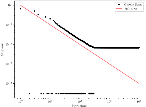
The effect of δ. In our original experiment on the RockPaper-Scissor game we set δ = 10-8 , which can also be deduced by the "small steps" in Figure 2 (due to binary search, those were 2-28 ). To show that the algorithm indeed gets stuck in approximate equilibrium point, we repeat the experiment with δ = 10-4 . The results are presented in Figure 3. Notice how the duality gap plateaus a bit under 10-2 = O(√δ). This phenomenon aligns with the statement of Theorem 1, when not accounting for the constant κA.
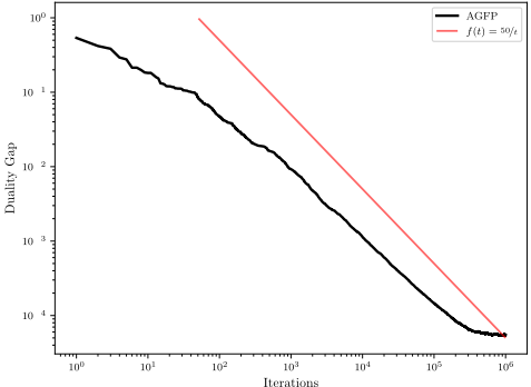
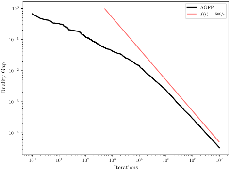
Performance in randomgames. Wemove forward by testing our method in randomly generated games. More specifically, we sample the entries of the matrix independently from a standard Gaussian distribution and normalize them in [0, 1]. Since we have already tested the "small" Rock-PaperScissors game, we first test at a moderate game of size 50×50 using δ = 10-8 . The results are presented in Figures 4 and 5. At first sight, it seems that the convergence of O( 1 T ) fails. However, upon closer inspection, we can see that the line gets parallel with the previous reference, until we approach the point of plateauing (around 10-4 ).
Before exploring further the effect of the dimension in the dynamics, we have to comment about the optimal steps in the random case. We observe that the nice picture of the RockPaper-Scissors games changes: the stepsizes are still decreasing, but they do not fit the line 1/t well. Still, it seems as they are distributed around it.
Iterations
Iterations
Figure 4: AGFP in a 50 × 50 random Gaussian game
The effect of the dimension. In the Rock-Paper-Scissors game, which is 3 × 3, we experimentally observed the rate to be 1 T . Then, in the 50 × 50 random Gaussian game we observe 50 T . We increase the dimension of the experiment by an order of magnitude and test our method on a 500 × 500 Gaussian game, setting δ = 10-11 and increasing the number of iterations to get a clearer image. Indeed, in Figure 6 we once again see a rate that scales as O( n T ). While all the illustrations presented here are for square matrices, we observed that in the non-square case, the duality gap scales with the maximum of the dimension.
About κA. The final remark of this section is that in all our random game experiments the convergence seems slow at first but then accelerates to match n T . This phenomenon matches our prediction when discussing κ after its Definition.
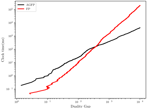
Wall-clock time. Standard Fictitious Play is observed to converge at a rate O( 1 √T ). Our proposed method improves this rate, but at the expense of increased computational overhead per iteration. To assess whether this trade-off yields a net benefit in practice, we benchmark the wall-clock timeto-accuracy performance of both algorithms. The results are presented in Figure 7 for a 50 × 50 Gaussian game with δ = 10-10 . We observe that already at an approximation of 10-3 our algorithm is faster, while for 10-4 the difference is striking. The classical algorithm requires around 195 seconds, while our method just over 4, a 50× improvement.
5 Discussion and FutureWork
We began our exploration with the Rock-Paper-Scissors game. It is only natural to conclude with it. We start with the standard 3 × 3 game. Note that under our symmetric and pure initialization, the only time where the best response was unique was at the first step. At any other time, two of three strategies yielded the same playoff, since all three can only occur at the equilibrium. We conjecture that if the algorithm had memory, then the tie-breaking where it picks a different best response than the previous iteration converges at the rate of 1 T with the stepsize sequence η∗ 1 = 2/3 and η∗ t = 1/t, t ≥ 2.
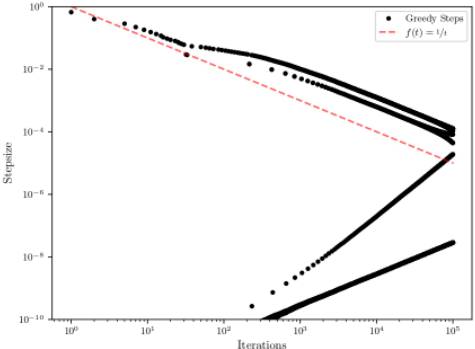
Now, the next interesting question is whether that sequence is the optimal one for RPS in higher dimensions. The immediate answer is negative, but there is more to that. In Figure 8 we present the steps the algorithm selects for an RPS game in higher dimension, where we clipped the noisy steps due to δ = 10-11 . We still see a decreasing line that is close to 1/t but now there are two increasing straight lines as well. We do not have a theoretical justification for this phenomenon and leave it as an open question. Another avenue for future work is to study our algorithm, and especially the condition-like number, in the smooth regime. [Anagnostides and Sandholm, 2024] provided a similar treatment to gradient-based algorithms. Finally, we must note that interesting pursuits are to adapt our idea to non zero-sum games. It seems especially promising to explore the direction of potential games. Since those games admit a pure Nash equilibrium, once the best response direction is this point, our algorithmwill jump to it.
Acknowledgments
We would like to thank Michail Fasoulakis, Ioannis Kakatelis and Nikoleta Sevastaki for useful discussions. This work was partially supported by the framework of the H.F.R.I call "Basic research Financing (Horizontal support of all Sciences)" under the National Recovery and Resilience Plan "Greece 2.0" funded by the European Union - NextGenerationEU (H.F.R.I. Project Number: 15877) and by the project MIS 5154714 of the National Recovery and Resilience Plan "Greece 2.0" funded by the European Union under the NextGenerationEU Program.
@inproceedings{ijcai2026p390,
  title     = {Do Not Discretize, Optimize: Almost Greedy Fictitious Play},
  author    = {Markakis, Evangelos and Santorinaios, Christodoulos},
  booktitle = {Proceedings of the Thirty-Fifth International Joint Conference on
               Artificial Intelligence, {IJCAI-26}},
  publisher = {International Joint Conferences on Artificial Intelligence Organization},
  editor    = {Diego Calvanese},
  pages     = {3505--3513},
  year      = {2026},
  month     = {8},
  note      = {Main Track},
  doi       = {10.24963/ijcai.2026/390},
  url       = {https://doi.org/10.24963/ijcai.2026/390},
}
TY - CPAPER TI - Do Not Discretize, Optimize: Almost Greedy Fictitious Play AU - Markakis, Evangelos AU - Santorinaios, Christodoulos T2 - Proceedings of the Thirty-Fifth International Joint Conference on Artificial Intelligence, IJCAI-26 PB - International Joint Conferences on Artificial Intelligence Organization PY - 2026 SP - 3505 EP - 3513 DO - 10.24963/ijcai.2026/390 UR - https://doi.org/10.24963/ijcai.2026/390 ER -Copied
Machine-readable versions of this paper, for tools and AI agents:





