
Identification of Probabilities of Causation: From Recursive to Closed-Form Bounds
Proceedings of the Thirty-Fifth International Joint Conference on Artificial Intelligence. Main Track. Pages 4063-4070.
https://doi.org/10.24963/ijcai.2026/452
Keywords
- Uncertainty in AI: Causality, structural causal models and causal inference
- Knowledge Representation and Reasoning: Causality
- Uncertainty in AI: Graphical models
Abstract
Probabilities of causation (PoCs) are fundamental quantities for counterfactual analysis and personalized decision making. However, existing analytical results are largely confined to binary settings. This paper extends PoCs to multi-valued treatments and outcomes by deriving closed form bounds for a representative family of discrete PoCs within Structural Causal Models, using standard experimental and observational distributions. We introduce the notion of equivalence classes of PoCs, which reduces arbitrary discrete PoCs to this family, and establish a replaceability principle that transfers bounds across value permutations. For the resulting bounds, we prove soundness in all dimensions and empirically verify tightness in low dimensional cases via Balke's linear programming method; we further conjecture that this tightness extends to all dimensions. Simulations indicate that our closed form bounds consistently tighten recent recursive bounds while remaining simpler to compute. Finally, we illustrate the practical relevance of our results through toy examples.
- [Balke, 1995] Alexander Abraham Balke. Probabilistic counterfactuals: semantics, computation, and applica- tions. University of California, Los Angeles, 1995.
- [Dawid et al., 2017] A Philip Dawid, Monica Musio, and Rossella Murtas. The probability of causation. Law, Prob- ability and Risk, 16(4):163-179, 2017.
- [de Aguas et al., 2025] Johan de Aguas, Sebastian Krum- scheid, Johan Pensar, and Guido Biele. The probability of tiered benefit: Partial identification with robust and stable inference. arXiv preprint arXiv:2502.10049, 2025.
- [Galles and Pearl, 1998] David Galles and Judea Pearl. An axiomatic characterization of causal counterfactuals. Foundations of Science, 3:151-182, 1998.
- [Halpern, 2000] Joseph Y Halpern. Axiomatizing causal reasoning. Journal of Artificial Intelligence Research, 12:317-337, 2000.
- [Li and Pearl, 2019] Ang Li and Judea Pearl. Unit selec- tion based on counterfactual logic. In Proceedings of the Twenty-Eighth International Joint Conference on Artificial Intelligence, 2019.
- [Li and Pearl, 2022a] Ang Li and Judea Pearl. Bounds on causal effects and application to high dimensional data. In Proceedings of the AAAI Conference on Artificial Intelli- gence, volume 36, pages 5773-5780, 2022.
- [Li and Pearl, 2022b] Ang Li and Judea Pearl. Unit selec- tion with causal diagram. In Proceedings of the AAAI con- ference on artificial intelligence, volume 36, pages 5765- 5772, 2022.
- [Li and Pearl, 2024] Ang Li and Judea Pearl. Probabilities of causation with nonbinary treatment and effect. In Pro- ceedings of the AAAI Conference on Artificial Intelligence, volume 38, pages 20465-20472, 2024.
- [Mueller and Pearl, 2022] Scott Mueller and Judea Pearl. Personalized decision making -a conceptual introduction. Technical Report R-513, Department of Computer Sci- ence, University of California, Los Angeles, CA, 2022.
- [Mueller et al., 2021] Scott Mueller, Ang Li, and Judea Pearl. Causes of effects: Learning individual responses from population data. arXiv preprint arXiv:2104.13730, 2021. IJCAI
- [Mueller, 2025] Scott Mueller. Personalized and Situation- Specific Decision Making. University of California, Los Angeles, 2025.
- [Pearl, 1999] Judea Pearl. Probabilities of causation: Three counterfactual interpretations and their identification. Syn- these, pages 93-149, 1999.
- [Tian and Pearl, 2000] Jin Tian and Judea Pearl. Probabil- ities of causation: Bounds and identification. Annals of Mathematics and Artificial Intelligence, 28(1-4):287-313, 2000.
- [Zhang et al., 2022] Junzhe Zhang, Jin Tian, and Elias Bareinboim. Partial counterfactual identification from observational and experimental data. In International Conference on Machine Learning, pages 26548-26558.
- PMLR, 2022.
References were extracted automatically from the PDF and may contain errors.
Full text extracted automatically from the PDF; figures, tables and equations may differ. The PDF is the version of record.
1 Introduction
In fields such as healthcare, finance, and energy, probabilities of causation can enable effective, accurate, and explainable decision-making in complex scenarios. This causalitybased approach addresses key challenges, including selection bias, counterfactual reasoning, individualized decisionmaking, and proper credit assignment-ensuring that outcomes are attributed to the treatments or factors that actually caused them. For example, Li and Pearl [2019] proposed a unit selection framework that uses a linear combination of probabilities of causation to identify individuals who are most likely to respond as desired, while also evaluating the associated rewards and costs. Similarly, Mueller and Pearl [2022] demonstrated how probabilities of causation can guide personalized medical decisions in alignment with the ethical principle of "do no harm."
The development of probabilities of causation began in the early 2000s, when Pearl [1999] first introduced three key binary measures: the probability of necessity (PN), the probability of sufficiency (PS), and the probability of necessity and sufficiency (PNS) in the Structural Causal Models (SCMs) [Galles and Pearl, 1998; Halpern, 2000]. Tian and Pearl [2000] then derived tight bounds for these quantities using Balke's linear programming method [Balke, 1995]. Decades later, Li and Pearl [2019; 2022b] formally proved the validity of these bounds. Building on this foundation, Muller et al. [2021], along with Dawid et al. [2017], further narrowed the bounds by incorporating covariate information and leveraging underlying causal structures.
The aforementioned studies are all restricted to binary treatments and outcomes, which poses significant limitations for real-world applications. In contrast, extending probabilities of causation to the non-binary case enables a more detailed and informative assessment. For example, in a binary setting, physicians can only determine whether a medication is effective or not, leading to a simple yes-or-no prescription decision. However, with multi-valued treatments xi (e.g., different dosage levels, where 1 ≤ i ≤ n and n ∈ N), doctors can evaluate which dosage level yields the optimal therapeutic effect for a particular patient. This finer-grained understanding supports more personalized and effective treatment decisions.
Efforts to address non-binary cases have continued in recent work. Zhang et al. [2022], as well as Li and Pearl [2022a], proposed numerical methods for computing nonbinary probabilities of causation using nonlinear programming techniques.
More recently, Li and Pearl [2024] introduced recursiveform but un-tight theoretical bounds for non-binary probabilities. Relatedly, de Aguas et al. [2025] studied probabilities of tiered benefit and harm for ordinal outcomes, focusing on cross-threshold causal effects and semiparametric inference. Despite these advances, existing approaches still face important limitations: numerical methods can become computationally demanding as the numbers of treatment and outcome values grow, while recursive analytical bounds may lose sharpness through repeated bounding steps. This lack of sharpness can directly affect downstream decision-making, since bounds that straddle a meaningful decision threshold may leave the relevant conclusion unresolved.
To address these limitations, we derive closed-form, nonrecursive bounds for arbitrary non-binary probabilities of causation in general SCMs, using standard experimental and observational distributions. Our approach first identifies a representative family of non-binary PoCs that is sufficient to express arbitrary discrete PoC queries, and then derives bounds for this family through equivalence classes and a replaceability principle. We prove the soundness of the proposed bounds in all dimensions and empirically verify their tightness in low-dimensional cases, specifically when the treatment and outcome take three or four possible values, using Balke's linear programming framework [Balke, 1995]. While a complete proof of tightness in the general n-dimensional case remains open.
1.1 Key Contributions
- We derive closed-form bounds for multi-valued PoCs in SCMs from only experimental and observational data.
- We introduce equivalence classes and a replaceability principle to reduce arbitrary PoC queries and transfer bounds across value permutations.
- We prove soundness for all dimensions, verify tightness in low dimensions, and show consistent tightening over Li-Pearl method with improved computational simplicity.
2 Preliminaries
We begin by reviewing the basic definitions of probabilities of causation and the associated notation in Structural Causal Models (SCMs) [Galles and Pearl, 1998; Halpern, 2000]. Readers already familiar with SCMs may choose to skip this section.
Counterfactuals are well defined within the SCM framework. A counterfactual statement such as "Variable Y would have the value y had X been x" is denoted as Yx = y. Here, the subscript x refers to a hypothetical event, which is welldefined in SCMs. For brevity, we will use yx, yx′ , y′x , and y′x′ throughout the paper to represent the events Yx = y, Yx′ = y, Yx = y′ , and Yx′ = y′ , respectively. Unless otherwise specified, we assume that experimental data are available in the form of causal effects (e.g., P(yx)), while observational data are provided as joint probabilities (e.g., P(x, y)). In our notation, X denotes the treatment variable and Y denotes the outcome or effect.
Let X and Y be two binary variables in a causal model M, where x denotes the proposition X = true, x′ denotes X = false, y denotes Y = true, and y′ denotes Y = false. The three basic binary probabilities of causation-PN, PS, and PNS-are defined as follows [Pearl, 1999]:
Definition 1 (Probabilities of Causation). [Pearl, 1999]
PNS stands for the probability that y would respond to x both ways, and therefore measures both the sufficiency and necessity of x to produce y.
Tian and Pearl [2000] then derived tight bounds for the PN, PS, and PNS using Balke's linear programming approach [Balke, 1995]. These bounds were later given a formal theoretical proof by Li and Pearl [2019; 2022b].
The tight bounds for binary PNS, PN, and PS, are given as follows:
Regarding non-binary probabilities of causation, Li and Pearl [2024] recently provided eight theorems establishing theoretical (though not tight) recursive-form bounds for cases where both the treatment and the effect are non-binary. Specifically, when the treatment variable X takes m values and the outcome variable Y takes n values, the following set of non-binary probabilities of causation are defined and bounded. (We omit the detailed bounds here; interested readers may refer to [Li and Pearl, 2024] for full derivations.)
Probability of preservation(i, j):
Probability of replacement(i, j, k):
Probability of substitute(i, j, k):
Probability of necessity(i, j, k, p):
Probability of necessity and sufficiency(k):
Probability of substitute(k,p):
Probability of replacement(k,q):
Probability of necessity(k, p, q):
In this paper, we will provide tighter bounds for a subset of the modified probabilities defined above and demonstrate that these selected probabilities are sufficient to represent all discrete probabilities of causation within SCMs.
3 Main Results
In this section, we first simplify the definitions of the Probability of Necessity and Sufficiency(k), Probability of Substitute(k,p), Probability of Replacement(k,q), and Probability of Necessity(k,p,q) defined by Li and Pearl [2024] into their most concise forms, while retaining their ability to represent all discrete probabilities of causation in Structural Causal Models (SCMs).
3.1 Probability of necessity and sufficiency(k)
The Probability of Necessity and Sufficiency(k) is simplified to the form P(y1x1 , . . . , ykxk ), where |X| = |Y | = n, the cardinalities of the state spaces of X and Y are both n, and the values of X and Y are arranged in increasing order within the probability expression. This simplification yields the most straightforward closed-form representation. We will later demonstrate that this simplification preserves generality. The closed-form bounds for the modified Probability of Necessity and Sufficiency(k) are presented in the following theorem. All theorem proofs are provided in the appendix.
Theorem 2 (Probability of necessity and sufficiency(k) (PNS(k))). Suppose variable X has n values x1, ..., xn and Y has n values y1, ..., yn, k ≤ n, then the probability of necessity and sufficiency(k) P (y1x1 , ..., ykxk ) is bounded as following:
Note that PNS(k) is a nonbinary, higher-order generalization of the original PNS. For example, PNS(2)-which reduces to the binary PNS-represents the probability that y1 would respond to x1 and y2 would respond to x2, formally written as P(y1x1 , y2x2 ). Bounds for similar probabilities, such as P(y2x1 , y1x2 ), can also be derived by leveraging the replaceability property of the probabilities of causation, as described in Theorem 7.
The proof of soundness, specifying when the bounds are attained with equality, is provided in the appendix. We will also present toy examples to illustrate how our results enhance decision-making capabilities. While some may argue that the previous definition of PNS(k) is more general, we will later demonstrate their equivalence in expressive power in Theorem 6.
3.2 Probability of substitute(k, p)
Similar to the Probability of Necessity and Sufficiency(k), the Probability of Substitute(k, p) is simplified as stated in the following theorem:
Theorem 3 (Probability of substitute(k, p) (PSub(k, p))). Suppose variable X has n values x1, ..., xn and Y has n values y1, ..., yn, k ≤ n, then the probability P(y1x1 , ..., ykxk , xp), s.t., p ̸= j for 1 ≤ j ≤ k is bounded as following:
3.3 Probability of replacement(k, q)
Then, the Probability of replacement(k, q) is simplified as stated in the following theorem:
Theorem 4 (Probability of replacement(k, q) (PRep(k, q))). Suppose variable X has n values x1, ..., xn and Y has n values y1, ..., yn, k ≤ n, then the probability P(y1x1 , ..., ykxk , yq) is bounded as following:
3.4 Probability of necessity(k, p, q)
Finally, the Probability of necessity(k, p, q) is simplified as stated in the following theorem:
Theorem 5 (Probability of necessity(k, p, q) (PN(k, p, q))). Suppose variable X has n values x1, ..., xn and Y has n values y1, ..., yn, k ≤ n, then the probability P(y1x1 , ..., ykxk , xp, yq), s.t., p ̸= j for 1 ≤ j ≤ k is bounded as following:
3.5 Equivalence Class in Probability of Causation
We now proceed to demonstrate the generality of the above modified probabilities of causation through the next two theorems.
Theorem 6 (Equivalence classes in probabilities of causation). Suppose variable X has n values x1, ..., xn, Y has m values y1, ..., ym:
- Case 1: Let Y ′ have n values y′1 , ..., y′n . W.L.O.G., let k ≤ m < n.
Then the bounds of the probability, P(y1x1 , ..., ykxk ), is exactly the same as the bounds of the probability, P (y′1x1 , ..., y′kxk ), where
and,
- Case 2: Let X′ have m values x′1 , ..., x′m. W.L.O.G., let k ≤ m < n.
Then the bounds of the probability, P(y1x1 , ..., ykxk ), is exactly the same as the bounds of the probability, P (y′1x1 , ..., y′kxk ), where
and,
3.6 Replaceability in Probability of Causation
Theorem 7 (Replaceability in probabilities of causation). Suppose variable X has n values x1, ..., xn and Y has n values y1, ..., yn, then the bounds of the probability, P(y1x1 , ..., yi-1xi-1 , yˆixi , yi+1xi+1 , ..., ykxk ), can be obtained by replacing yixi with yˆixi for any i, such that 1 ≤ i,ˆi ≤ n, in the bounds of the probability, P(y1x1 , ..., ykxk ).
Note that both theorems apply to the cases of PNS(k), Psub(k, p), PRep(k, q), and PN(k, p, q). For instance, to derive the bounds for P(yx, yx′ , y′′ x′′ | x′′′ , y′′′ ), we can first apply PN(3, 4, 4) to obtain P(yx, y′x′ , y′′ x′′ , x′′′ , y′′′ ). If |X| ̸= |Y |, we should first apply Theorem 6. Then, using the replaceability property of probabilities of causation (Theorem 7), we can convert P(yx, y′x′ , y′′ x′′ , x′′′ , y′′′ ) into P (yx, yx′ , y′′ x′′ , x′′′ , y′′′ ). Finally, dividing by P(x′′′ , y′′′ ) yields the desired conditional probability: P(yx, yx′ , y′′ x′′ | x′′′ , y′′′ ).
4 Examples
In this section, we will discuss several examples to demonstrate the effectiveness and usefulness of our results.
4.1 Cross-Treatment Heterogeneity inMedicine
Consider patients with hypertension who are eligible for three alternative treatment options. Standard clinical summaries report average improvement rates for each treatment, yet they fail to identify patients who would benefit from one treatment but be harmed by another. Since the same patient cannot receive all treatments simultaneously, and responses observed at different times may be confounded by disease progression, such cross-treatment responses are inherently counterfactual, motivating the use of multi-valued probabilities of causation.
Let X denote the treatment assigned to a patient, where x1, x2, and x3 correspond to Treatment 1, Treatment 2, and Treatment 3, respectively. Let Y denote the clinical outcome category, with y1, y2, and y3 indicating poor outcome, moderate outcome, and good outcome.
We focus on the probability of causation P(y3x1 , y1x2 , y2x3 ), which quantifies the fraction of patients who would achieve a good outcome under Treatment 1, a poor outcome under Treatment 2, and only a moderate outcome under Treatment 3. Such cross-treatment response patterns cannot be inferred from marginal outcome rates alone.
To obtain the required estimates, clinicians conduct a randomized clinical trial with 900 patients, where each patient is assigned to one of the three treatments. The experimental data are summarized in Table 1.
| Treatment 1 | Treatment 2 | Treatment 3 | |
|---|---|---|---|
| poor | 46 | 270 | 40 |
| moderate | 23 | 8 | 223 |
| good | 231 | 22 | 37 |
| Overall | 300 | 300 | 300 |
Notably, each marginal experimental probability appearing in the target conjunction, namely P(y3x1 ), P(y1x2 ), and P(y2x3 ), exceeds 0.5. This might suggest that the joint probability P(y3x1 , y1x2 , y2x3 ) is also large. However, this inference is not justified without causal bounds that account for cross-world dependencies.
In addition, clinicians collected observational data from 900 patients whose treatment choices were self-selected, as summarized in Table 2.
By plugging both the experimental and observational data into Theorem 2 together with the replaceability property (Theorem 7), we obtain the following bounds:
In contrast, the recursive bounds obtained using the method of Li and Pearl [2024] yield [0.428, 0.588], which leaves substantial ambiguity as to whether this response type constitutes a majority of patients.
Our tighter lower bound resolves this ambiguity by showing that more than half of patients exhibit this cross-treatment response pattern, indicating a large subgroup for which Treatment 1 is beneficial, Treatment 2 is harmful, and Treatment 3 is intermediate. Such risk-relevant heterogeneity is invisible to marginal outcome comparisons and highlights how tighter multi-valued PoC bounds can guide heterogeneityaware treatment selection.
4.2 Personalized Decision-Making in Educational Interventions
An education platform provides academic support at multiple intensity levels for learners preparing for certification exams. While the platform advertises that increased instructional intensity leads to better learning outcomes on average, advisors are concerned that overly aggressive intervention may harm some learners.
Consider a learner with stable but unexceptional performance. The advisor seeks to assess whether moderate support would be beneficial, while intensive support could instead be detrimental. Such questions are central to personalized education policy, where one-size-fits-all strategies may be suboptimal.
| Treatment 1 | Treatment 2 | Treatment 3 | |
|---|---|---|---|
| poor | 131 | 45 | 38 |
| moderate | 68 | 22 | 483 |
| good | 1 | 51 | 61 |
| Overall | 200 | 118 | 582 |
| Intensive | Moderate | Light | None | |
|---|---|---|---|---|
| Fail | 195 | 11 | 80 | 100 |
| Pass | 51 | 266 | 198 | 147 |
| Excellent | 54 | 23 | 22 | 53 |
| Overall | 300 | 300 | 300 | 300 |
Let X denote the level of academic support, ranging from intensive (x1), moderate (x2), light (x3) to none (x4). Let Y denote the learner's grade at the end of the term, where y1 indicates fail the exam (e.g., grade F), y2 indicates pass the exam, and y3 indicates excellent performance (e.g., grade A).
The advisor's query is captured by the probability of causationP(y1x1 , y2x2 , y2x3 | x4, y2), which asks: among learners who currently pass without support, what is the probability that they would still pass under light or moderate support, but fail under intensive intervention?
To answer this question, the advisor obtains historical data collected by the platform over several academic terms, during which learners participated in different intensity levels while following comparable curricula and assessment standards. The data include both experimental studies (where 1200 learners were assigned to different intervention levels) and observational records (where 1200 learners self-selected their level of support). These results are summarized in Tables 3 and 4.
Based on an observational study, the platform reports that higher levels of intervention are associated with improved performance on average: 16.1%, 7.3%, 5.8%, and 3.2% of learners achieve excellent performance under intensive instruction, moderate instruction, light instruction, and no additional support, respectively, suggesting that intensive training may be beneficial. However, such averages do not address individual-level risks.
We therefore consider:
which quantifies the probability that increasing intervention intensity would negatively affect learners who are currently stable without support.
Applying the experimental and observational estimates to Theorem 5 and Theorem 7, we obtain:
| Intensive | Moderate | Light | None | |
|---|---|---|---|---|
| Fail | 67 | 11 | 53 | 46 |
| Pass | 129 | 17 | 53 | 436 |
| Excellent | 193 | 87 | 70 | 38 |
| Overall | 389 | 115 | 176 | 520 |
which is strictly tighter than the bounds obtained using the method of Li and Pearl [2024]: [0, 0.363].
Since P(x4, y2) = 436 1200 , this yields:
which is substantially more informative than the vacuous bound [0, 1] obtained by Li and Pearl [2024] method.
These results allow academic advisors to conclude that, for a non-negligible subset of learners, intensive intervention poses a significant risk of adverse outcomes, while moderate support remains safe.
5 Simulated Results
In this section, we empirically demonstrate that the conjectured closed-form bounds yield tighter estimates than the recursive bounds of Li and Pearl [2024]. Here we focus on the probability of necessity and sufficiency (PNS) to provide a simple and visually direct illustration of how much improvement is obtained in practice. Our generated data satisfy the consistency relation between experimental and observational distributions. We uniformly generate each interventional distribution P(Yxj = yi) first, and then uniformly generate observational distributions subject to compatibility constraints with the experimental data. In particular, following Tian-Pearl's bounds, for any i, j ∈ {1, . . . , n}, we require P(xj , yi) ≤ P(yixj ) ≤ 1 - P(xj , yi′ ), for all i′ ̸= i.
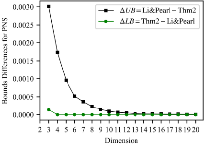
Dimension sweep (n ∈ [3, 20]). We fix k = 3 (i.e., X and Y each take three values) and vary the dimensionality n ∈ [3, 20], focusing on the probability of necessity and sufficiency PNS(k). For each n, we randomly generate 10,000 ground-truth instances of PNS(3), i.e., P(y1x1 , y2x2 , y3x3 ). For every instance, we construct compatible observational and experimental sample distributions. Our data-generation procedure enforces the standard feasibility constraint P(xi, yi) ≤ P(yixi ) ≤ 1-P(xi)+P(xi, yi). For each n, we compute the average improvement of our bounds over the 10,000 instances and plot the resulting differences in Figure 1. Across all dimensions, the improvements are never negative. Moreover, the average improvement decreases as n increases, which is expected because probability mass is spread over more categories, making typical values of P (xi, yi) and P (yixi ) smaller.
| n, k | Avg. inc. LB | Avg. dec. UB | Li-Pearl PNS gap | Thm. 2 PNS gap | Bounds narrower |
|---|---|---|---|---|---|
| 3, 3 | 0.0002 | 0.0029 | 0.1691 | 0.1661 | 1737 |
| 4, 4 | 0.0000 | 0.0024 | 0.1006 | 0.0983 | 1652 |
| 5, 5 | 0.0000 | 0.0018 | 0.0669 | 0.0651 | 1628 |
| 5, 4 | 0.0000 | 0.0015 | 0.0789 | 0.0775 | 1186 |
| 4, 3 | 0.0000 | 0.0018 | 0.1257 | 0.1239 | 1088 |
| 5, 3 | 0.0000 | 0.0009 | 0.0952 | 0.0943 | 746 |
Per-instance comparisons. To further illustrate the improvement at the level of individual instances, we consider several representative settings, n ∈ {3, 4, 5}, k ∈ {3, 4, 5} (chosen for convenience of presentation). For each setting, we generate 10,000 compatible sample distributions and compute bounds by both methods. For sample i, let [ai, bi] denote the bounds from our theorem and [ci, di] denote the bounds from Li and Pearl [2024]. We summarize the following quantities:
- Average increase in the lower bound : ∑ (ai-ci) 10000
- Average decrease in the upper bound : ∑ (di-bi) 10000
- Average gap from Li and Pearl: ∑ (di-ci) 10000
- Average gap from theorem 2 : ∑ (bi-ai) 10000
- Count of sample distributions where Theorem 2 yields narrower bounds : ∑ fi where, fi = 1 if (ai > ci) or (bi < di) and fi = 0 otherwise.
Table 5 reports these summary statistics across different dimensions. Notably, the bounds are narrowed in approximately 10%-20% of the samples.
Visualizing per-instance improvements. To complement the aggregate trends in Fig. 1 and the summary statistics in Table 5, we further examine per-instance behavior to illustrate how bound tightening manifests at the level of individual samples across dimensions.
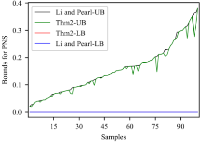
Figure 2: PNS bounds over 100 instances for n = k = 3.
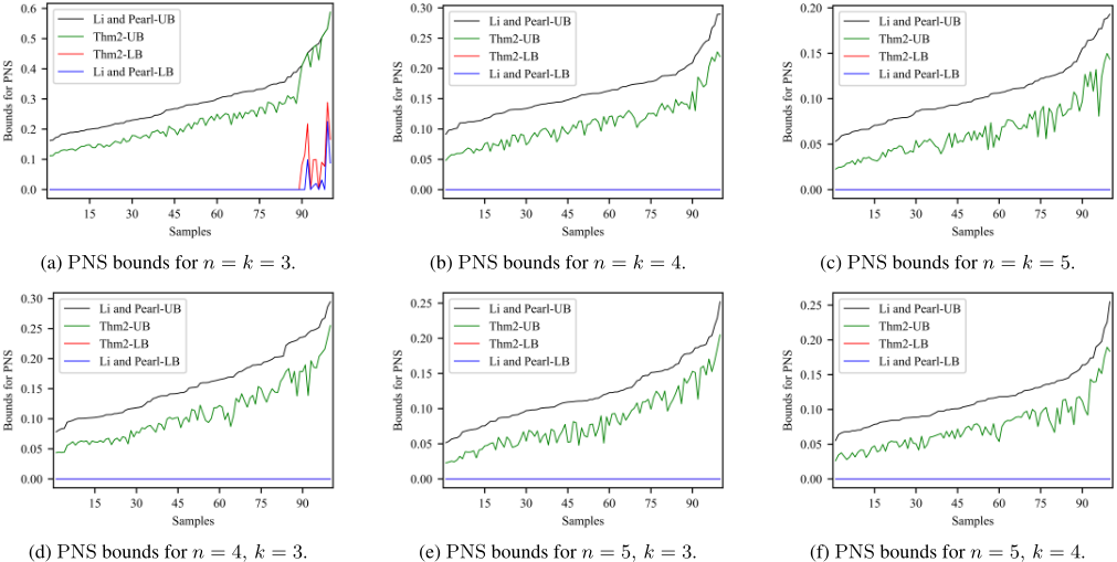
Figure 2 shows the lower and upper bounds for 100 representative instances with n = k = 3, comparing the bounds from Theorem 2 and from Li and Pearl [2024]. Extending this analysis, Fig. 3 reports results across multiple (n, k) settings. For each configuration, we generate 10,000 compatible sample distributions and select the 100 instances with the largest discrepancies between the two methods, ordered by their PNS bounds to facilitate comparison.
As dimensionality increases, the lower bounds increasingly concentrate near zero. This behavior is expected, since probability mass is spread over a larger number of categories, reducing typical values of terms such as P(xi, yi) and P(yixi ), and thereby limiting potential improvements in the lower bounds.
Importantly, this does not diminish the advantage of the proposed approach. Instead, with increasing n, the relative separation between the bounds produced by Theorem 2 and those of Li and Pearl becomes more pronounced, driven mainly by systematic reductions in the upper bounds. This trend is particularly evident in Fig. 3a-3c, where n = k and the relative gap widens as dimensionality grows.
Moreover, Fig. 3d-3f show that this separation persists when n ̸= k, indicating that the closed-form bounds remain accurate beyond the diagonal (n = k) regime. Overall, these results demonstrate that the proposed closed-form expressions are not only computationally simpler, but also consistently tight across a wide range of dimensional configurations.
6 Conclusion
We studied multi-valued probabilities of causation (PoCs) in general Structural Causal Models using experimental and observational distributions, without imposing structural restrictions. Our main contribution is a closed-form framework that reduces arbitrary discrete PoCs to a representative family with analytically derived bounds. Equivalence classes and replaceability transfer these bounds across value permutations and mismatched treatment-outcome cardinalities, yielding a compact toolkit for non-binary PoCs.
We established soundness in all dimensions and empirically verified tightness in low-dimensional settings via Balke's linear programming when feasible. Simulations show that our bounds consistently tighten the recursive bounds of Li and Pearl [2024] while being simpler to compute and suitable for repeated queries. These results suggest that the proposed bounds may be complete in general, although a formal tightness proof for all dimensions remains open.
Our examples show that multi-valued PoCs capture crossworld response patterns that marginal comparisons cannot reveal. In both medical and educational settings, they quantify latent response types-such as individuals who benefit under one intervention but may be harmed under another-thereby supporting heterogeneity-aware and personalized decisions.
Several open directions remain. A general completeness proof is still open beyond the low-dimensional cases verified here. Future work may incorporate covariates and causal graphs to sharpen identification, and seek interpretable nonbinary structural assumptions for stronger bounds. In particular, extending monotonicity-type ideas such as Monotonic Incremental Treatment Effect (MITE) [Mueller, 2025] under partial-order constraints is a promising direction.
@inproceedings{ijcai2026p452,
  title     = {Identification of Probabilities of Causation: From Recursive to Closed-Form Bounds},
  author    = {Shu, Xin and Wang, Shuai and Li, Ang},
  booktitle = {Proceedings of the Thirty-Fifth International Joint Conference on
               Artificial Intelligence, {IJCAI-26}},
  publisher = {International Joint Conferences on Artificial Intelligence Organization},
  editor    = {Diego Calvanese},
  pages     = {4063--4070},
  year      = {2026},
  month     = {8},
  note      = {Main Track},
  doi       = {10.24963/ijcai.2026/452},
  url       = {https://doi.org/10.24963/ijcai.2026/452},
}
TY - CPAPER TI - Identification of Probabilities of Causation: From Recursive to Closed-Form Bounds AU - Shu, Xin AU - Wang, Shuai AU - Li, Ang T2 - Proceedings of the Thirty-Fifth International Joint Conference on Artificial Intelligence, IJCAI-26 PB - International Joint Conferences on Artificial Intelligence Organization PY - 2026 SP - 4063 EP - 4070 DO - 10.24963/ijcai.2026/452 UR - https://doi.org/10.24963/ijcai.2026/452 ER -Copied
Machine-readable versions of this paper, for tools and AI agents:





