
Counterfactual Estimation via Temporal-Aware Intervention Networks
Proceedings of the Thirty-Fifth International Joint Conference on Artificial Intelligence. Main Track. Pages 4079-4087.
https://doi.org/10.24963/ijcai.2026/454
Keywords
- Machine Learning: Causality
- Knowledge Representation and Reasoning: Causality
- Uncertainty in AI: Causality, structural causal models and causal inference
Abstract
Accurate estimation of time-varying treatment effects is crucial for optimizing interventions in personalized medicine. However, observational data often contains complex confounding bias and temporal complexities, making counterfactual estimation challenging. We propose Counterfactual Estimation via Temporal-Aware Intervention Networks (TAIN), a novel model that introduces an Intervention-aware Functional Convolution kernel to emphasize the role of treatments and capture complex temporal treatment interactions. TAIN addresses confounding bias from a domain generalization perspective, approximating the unknown target domain using adversarial examples and incorporating Sharpness-Aware Minimization to derive a generalization bound. This approach is more suitable for longitudinal settings compared to existing methods inspired by domain adaptation techniques due to inherent differences between static and longitudinal contexts. Experiments on simulated datasets demonstrate TAIN's superior performance compared to state-of-the-art models for counterfactual estimation over time.
- [Bai et al., 2018] Shaojie Bai, J Zico Kolter, and Vladlen Koltun. An empirical evaluation of generic convolutional and recurrent networks for sequence modeling. arXiv preprint arXiv:1803.01271, 2018.
- [Ban et al., 2025a] Taiyu Ban, Lyuzhou Chen, Derui Lyu, Xiangyu Wang, Qinrui Zhu, and Huanhuan Chen. Llm- driven causal discovery via harmonized prior. IEEE Trans- actions on Knowledge and Data Engineering, 2025.
- [Ban et al., 2025b] Taiyu Ban, Changxin Rong, Xiangyu Wang, Lyuzhou Chen, Xin Wang, Derui Lyu, Qinrui Zhu, and Huanhuan Chen. Differentiable structure learning with ancestral constraints. In Forty-second International Conference on Machine Learning, 2025.
- [Bica et al., 2020a] Ioana Bica, Ahmed Alaa, and Mihaela Van Der Schaar. Time series deconfounder: Estimating treatment effects over time in the presence of hidden con- founders. In International conference on machine learn- ing, pages 884-895. PMLR, 2020.
- [Bica et al., 2020b] Ioana Bica, Ahmed M Alaa, James Jor- don, and Mihaela van der Schaar. Estimating counterfac- tual treatment outcomes over time through adversarially balanced representations. In International Conference on Learning Representations, 2020.
- [Chen et al., 2023] Yehu Chen, Annamaria Prati, Jacob Montgomery, and Roman Garnett. A multi-task gaussian process model for inferring time-varying treatment effects in panel data. In International Conference on Artificial In- telligence and Statistics, pages 4068-4088. PMLR, 2023.
- [Chen et al., 2025] Lyuzhou Chen, Taiyu Ban, Derui Lyu, Yijia Sun, Kangtao Hu, Xiangyu Wang, and Huanhuan Chen. Continuous structure constraint integration for ro- bust causal discovery. In The 28th International Confer- ence on Artificial Intelligence and Statistics, 2025.
- [Chevillon, 2007] Guillaume Chevillon. Direct multi-step estimation and forecasting. Journal of Economic Surveys, 21(4):746-785, 2007.
- [Cho et al., 2014] Kyunghyun Cho, Bart van Merrienboer, Dzmitry Bahdanau, and Yoshua Bengio. On the proper- ties of neural machine translation: Encoder-decoder ap- proaches. In Proceedings of SSST-8, Eighth Workshop on Syntax, Semantics and Structure in Statistical Transla- tion, page 103. Association for Computational Linguistics, 2014.
- [Foret et al., 2021] Pierre Foret, Ariel Kleiner, Hossein Mobahi, and Behnam Neyshabur. Sharpness-aware mini- mization for efficiently improving generalization. In Inter- national Conference on Learning Representations, 2021.
- [Frauen et al., 2023] Dennis Frauen, Tobias Hatt, Valentyn Melnychuk, and Stefan Feuerriegel. Estimating average causal effects from patient trajectories. In Proceedings of the AAAI Conference on Artificial Intelligence, pages 7586-7594, 2023.
- [Ganin et al., 2016] Yaroslav Ganin, Evgeniya Ustinova, Hana Ajakan, Pascal Germain, Hugo Larochelle, Franc ¸ois Laviolette, Mario March, and Victor Lempitsky. Domain- adversarial training of neural networks. Journal of ma- chine learning research, 17(59):1-35, 2016.
- [Geng et al., 2017] Changran Geng, Harald Paganetti, and Clemens Grassberger. Prediction of treatment response for combined chemo-and radiation therapy for non-small cell lung cancer patients using a bio-mathematical model. Scientific reports, 7(1):13542, 2017.
- [Goodfellow et al., 2015] Ian J. Goodfellow, Jonathon Shlens, and Christian Szegedy. Explaining and harnessing adversarial examples. In 3rd International Conference on Learning Representations, ICLR 2015, San Diego, CA, USA, May 7-9, 2015, Conference Track Proceedings, 2015.
- [Hariton and Locascio, 2018] Eduardo Hariton and Joseph J Locascio. Randomised controlled trials-the gold stan- dard for effectiveness research. BJOG: an international journal of obstetrics and gynaecology, 125(13):1716, 2018.
- [Hassanpour and Greiner, 2019] Negar Hassanpour and Russell Greiner. Counterfactual regression with impor- tance sampling weights. In IJCAI, pages 5880-5887, 2019. IJCAI
- [He et al., 2016] Kaiming He, Xiangyu Zhang, Shaoqing Ren, and Jian Sun. Deep residual learning for image recog- nition. In Proceedings of the IEEE conference on computer vision and pattern recognition, pages 770-778, 2016.
- [Hess et al., 2024] Konstantin Hess, Valentyn Melnychuk, Dennis Frauen, and Stefan Feuerriegel. Bayesian neu- ral controlled differential equations for treatment effect estimation. In The Twelfth International Conference on Learning Representations, 2024.
- [Huang and Ning, 2012] Xuelin Huang and Jing Ning. Anal- ysis of multi-stage treatments for recurrent diseases. Statistics in medicine, 31(24):2805-2821, 2012.
- [Huang et al., 2024] Qiang Huang, Chuizheng Meng, Defu Cao, Biwei Huang, Yi Chang, and Yan Liu. An empir- ical examination of balancing strategy for counterfactual estimation on time series. In Forty-first International Con- ference on Machine Learning, 2024.
- [Johansson et al., 2016] Fredrik Johansson, Uri Shalit, and David Sontag. Learning representations for counterfactual inference. In International conference on machine learn- ing, pages 3020-3029. PMLR, 2016.
- [Johansson et al., 2022] Fredrik D Johansson, Uri Shalit, Nathan Kallus, and David Sontag. Generalization bounds and representation learning for estimation of potential out- comes and causal effects. The Journal of Machine Learn- ing Research, 23(1):7489-7538, 2022.
- [Li et al., 2021] Rui Li, Stephanie Hu, Mingyu Lu, Yuria Utsumi, Prithwish Chakraborty, Daby M. Sow, Piyush Madan, Jun Li, Mohamed Ghalwash, Zach Shahn, and Li-wei Lehman. G-net: a recurrent network approach to g-computation for counterfactual prediction under a dynamic treatment regime. In Proceedings of Machine Learning for Health, volume 158 of Proceedings of Ma- chine Learning Research, pages 282-299. PMLR, 04 Dec 2021.
- [Lim et al., 2018] Bryan Lim, Ahmed Alaa, and Mihaela van der Schaar. Forecasting treatment responses over time using recurrent marginal structural networks. Advances in neural information processing systems, 31, 2018.
- [Matsuura and Harada, 2020] Toshihiko Matsuura and Tat- suya Harada. Domain generalization using a mixture of multiple latent domains. In Proceedings of the AAAI conference on artificial intelligence, pages 11749-11756, 2020.
- [Melnychuk et al., 2022] Valentyn Melnychuk, Dennis Frauen, and Stefan Feuerriegel. Causal transformer for estimating counterfactual outcomes. In International Conference on Machine Learning, pages 15293-15329.
- PMLR, 2022.
- [Meng et al., 2023] Chuizheng Meng, Yihe Dong, Sercan Ö Arık, Yan Liu, and Tomas Pfister. Costar: Improved tem- poral counterfactual estimation with self-supervised learn- ing. arXiv preprint arXiv:2311.00886, 2023.
- [Motiian et al., 2017] Saeid Motiian, Marco Piccirilli, Don- ald A Adjeroh, and Gianfranco Doretto. Unified deep su- pervised domain adaptation and generalization. In Pro- ceedings of the IEEE international conference on com- puter vision, pages 5715-5725, 2017.
- [Muandet et al., 2013] Krikamol Muandet, David Balduzzi, and Bernhard Schölkopf. Domain generalization via in- variant feature representation. In International conference on machine learning, pages 10-18. PMLR, 2013.
- [Nie et al., 2020] Lizhen Nie, Mao Ye, Dan Nicolae, et al. VCNet and functional targeted regularization for learning causal effects of continuous treatments. In Proceedings of the 9th International Conference on Learning Representa- tions, 2020.
- [Oord et al., 2016] Aaron van den Oord, Sander Diele- man, Heiga Zen, Karen Simonyan, Oriol Vinyals, Alex Graves, Nal Kalchbrenner, Andrew Senior, and Koray Kavukcuoglu. Wavenet: A generative model for raw au- dio. arXiv preprint arXiv:1609.03499, 2016.
- [Robins and Hernan, 2008] James Robins and Miguel Her- nan. Estimation of the causal effects of time-varying ex- posures. Chapman & Hall/CRC Handbooks of Modern Statistical Methods, pages 553-599, 2008.
- [Robins, 1986] James Robins. A new approach to causal inference in mortality studies with a sustained exposure period-application to control of the healthy worker sur- vivor effect. Mathematical modelling, 7(9-12):1393-1512, 1986.
- [Roemhild et al., 2022] Roderich Roemhild, Tobias Bollen- bach, and Dan I Andersson. The physiology and genetics of bacterial responses to antibiotic combinations. Nature Reviews Microbiology, 20(8):478-490, 2022.
- [Rubin, 1978] Donald B Rubin. Bayesian inference for causal effects: The role of randomization. The Annals of statistics, pages 34-58, 1978.
- [Seedat et al., 2022] Nabeel Seedat, Fergus Imrie, Alexis Bellot, Zhaozhi Qian, and Mihaela van der Schaar. Continuous-time modeling of counterfactual outcomes us- ing neural controlled differential equations. In Interna- tional Conference on Machine Learning, pages 19497- 19521. PMLR, 2022.
- [Shalit et al., 2017] Uri Shalit, Fredrik D Johansson, and David Sontag. Estimating individual treatment effect: gen- eralization bounds and algorithms. In International con- ference on machine learning, pages 3076-3085. PMLR, 2017.
- [Shi et al., 2021] Yuge Shi, Jeffrey Seely, Philip HS Torr, N Siddharth, Awni Hannun, Nicolas Usunier, and Gabriel Synnaeve. Gradient matching for domain generalization. arXiv preprint arXiv:2104.09937, 2021.
- [Taieb and Atiya, 2015] Souhaib Ben Taieb and Amir F Atiya. A bias and variance analysis for multistep-ahead time series forecasting. IEEE transactions on neural net- works and learning systems, 27(1):62-76, 2015.
- [Wang et al., 2024] Xin Wang, Shengfei Lyu, Lishan Yang, Yibing Zhan, and Huanhuan Chen. A dual-module frame- work for counterfactual estimation over time. In Forty-first International Conference on Machine Learning, 2024.
- [Wang et al., 2025] Xin Wang, Shengfei Lyu, Kangyang Luo, Lishan Yang, Huanhuan Chen, and Chunyan Miao. Enhancing counterfactual estimation: a focus on tempo- ral treatments. In Proceedings of the Thirty-Fourth Inter- national Joint Conference on Artificial Intelligence, pages 6442-6450, 2025. IJCAI
- [Xu et al., 2020] Minghao Xu, Jian Zhang, Bingbing Ni, Teng Li, Chengjie Wang, Qi Tian, and Wenjun Zhang. Ad- versarial domain adaptation with domain mixup. In Pro- ceedings of the AAAI conference on artificial intelligence, pages 6502-6509, 2020.
- [Zhang et al., 2024] Ruipeng Zhang, Ziqing Fan, Jiangchao Yao, Ya Zhang, and Yanfeng Wang. Domain-inspired sharpness-aware minimization under domain shifts. In The Twelfth International Conference on Learning Representa- tions, 2024.
References were extracted automatically from the PDF and may contain errors.
Full text extracted automatically from the PDF; figures, tables and equations may differ. The PDF is the version of record.
1 Introduction
Precise estimation of time-varying treatment effects is crucial in domains like personalized medicine, where optimizing individual interventions relies on accurate estimating counterfactual outcomes [Huang and Ning, 2012]. Randomized Controlled Trials, despite being the gold standard for causal inference [Hariton and Locascio, 2018], are limited by high costs and ethical concerns. Consequently, research has shifted focus to advanced methods tackling confounding bias and temporal complexities in observational data for accurate counterfactual estimation.
Time-varying confounders often introduce complex confounding bias in observational data, leading to inaccurate estimates. Recent studies [Bica et al., 2020b; Melnychuk et al., 2022; Wang et al., 2024] have addressed this issue by learning representations to break the association between historical information and treatment assignment, drawing inspiration from domain adaptation techniques used in static causal inference settings [Shalit et al., 2017; Hassanpour and Greiner, 2019; Johansson et al., 2022]. However, domain adaptation's effectiveness in longitudinal settings remains questionable due to inherent differences between the contexts.
Due to the unobservability of counterfactuals, we aim to train a model on the factual (source) domain that generalizes well to the counterfactual (target) domain. In static settings (Figure 1(a)), the target domain during testing is consistent with training and can be sampled, aligning with domain adaptation [Ganin et al., 2016]. However, in longitudinal settings, the historical information of length t generated under the training intervention policy (Figure 1(b)) differs from the τ -step intervened historical information under a different testing policy (Figure 1(c)). The unknown data generation process makes the target distribution unobservable during testing, possibly explaining why current balancing methods fail in longitudinal settings [Huang et al., 2024].
Another key challenge in longitudinal settings lies in modeling temporal treatment interactions. Take antibiotic treatments as an example - [Roemhild et al., 2022] have shown that the effectiveness of current antibiotics strongly depends on previously administered ones, making it critical to understand these temporal interactions for optimal treatment. While recent work ACTIN [Wang et al., 2024] attempts to capture such interactions using a dual-module architecture, it follows previous approaches [Bica et al., 2020b; Melnychuk et al., 2022] in treating treatments merely as regular inputs. This fails to emphasize treatments' special role in determining outcomes. Though the importance of emphasizing treatments has been demonstrated in static settings by VCNet [Nie et al., 2020], how to properly model treatment interactions over time remains an open challenge.
To address these challenges, we propose a novel model called Temporal-Aware Intervention Networks (TAIN) for counterfactual estimation over time. In order to emphasize the role that treatments play, we draw inspiration from VCNet, which allows the weights of the prediction head to be functions of the treatment. TAIN introduces an Interventionaware 1 Functional Convolution (IFC) kernel, ensuring that
1 In causal inference, "intervention" is a broad term. We primarily use "treatment" for medical interventions, although the terms are used interchangeably herein.
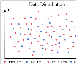
(a) Static setting
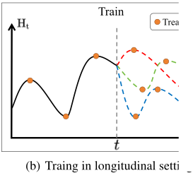
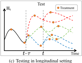
the convolutional kernel at each time step depends on the related treatment. Specifically, we employ Radial Basis Functions (RBFs) as basis functions to fit nonlinear functions of treatments, enhancing the model's ability to handle complex temporal treatment interactions. Furthermore, since the target domain is unobservable in longitudinal settings, we revisit confounding bias from the perspective of domain generalization. TAIN approximates the unknown target domain by generating adversarial examples using the Fast Gradient Sign Method (FGSM) [Goodfellow et al., 2015]. By incorporating Sharpness-Aware Minimization (SAM) [Foret et al., 2021], a technique for enhancing model generalization performance, we derive a generalization bound for the model under certain conditions. The objective function proposed based on this theoretical analysis can more effectively mitigate time-varying confounding bias. Our main contributions are summarized as follows:
- We propose a novel Intervention-aware Functional Convolution (IFC) kernel to capture complex temporal treatment interactions by designing convolutional kernels as functions of treatments.
- We revisit time-varying confounding bias from domain generalization perspective and derive a generalization bound using adversarial examples with SAM.
- Extensive experiments on synthetic datasets demonstrate TAIN's superior performance in counterfactual estimation over time.
2 ProblemFormulation
Consider an i.i.d. observational dataset D containing detailed information for N patients, denoted as D = {x(i) t , a(i) t , y(i) t T (i) t=1 ∪v(i)}N i=1 . For each patient i, we observe time-varying covariates X(i) t ∈ X, treatments A(i) t ∈ A, and outcomes Y(i) t ∈ Y at discrete time steps T (i) , along with static covariates V(i) ∈ V such as gender and age. For notational simplicity, we omit the patient-specific superscript (i) when the context is clear.
Building upon the potential outcome framework [Rubin, 1978] and its extension to time-varying treatments [Robins and Hernan, 2008], we aim to estimate time-varying counterfactual outcomes [Bica et al., 2020b; Lim et al., 2018; Li et al., 2021]. Let ¯Ht = ( ¯Xt, ¯At-1, ¯Yt,V) denote the patient's historical information, where ¯Xt = (X1, · · · ,Xt), ¯Yt = (Y1, · · · ,Yt), and ¯At-1 = (A1, · · · ,At-1). Our objective is to estimate the potential outcome Yt+τ [¯at:t+τ-1] following a treatment sequence ¯at:t+τ-1 = (at, · · · , at+τ-1), conditioned on the historical information ¯Ht:
To identify treatment effects from observational data, we rely on the assumptions of consistency, sequential ignorability, and sequential overlap, as established in prior works [Lim et al., 2018; Bica et al., 2020b; Melnychuk et al., 2022; Wang et al., 2024] and detailed in Appendix B.
3 RelatedWork
3.1 Causal inference with longitudinal data
Recently, significant progress has been made in the field of longitudinal data analysis by incorporating neural network techniques for counterfactual estimation. For instance, RMSN [Lim et al., 2018] combines two propensity networks and employs an inverse probability weighting (IPTW) based training method in its prediction model. G-Net [Li et al., 2021] enhances the traditional G-computation technique through a deep learning framework. Similarly, CRN [Bica et al., 2020b], which is also based on RNN networks, focuses on learning balanced representations to mitigate confounding bias. In contrast to these works, CT [Melnychuk et al., 2022] proposes utilizing a more powerful transformer model to better handle long-term dependencies, while ACTIN [Wang et al., 2024] introduces a dual-module framework that effectively enhances the ability of simple models to handle complex temporal treatment interactions. It is worth noting that CRN, CT, and ACTIN all adopt the idea of domain adaptation to learn balanced representations by eliminating the association between historical information and current treatment assignments to alleviate confounding bias.
X
Treatment
Time There have been significant advances in causal inference based on longitudinal data, albeit with different settings from ours [Bica et al., 2020a; Frauen et al., 2023; Seedat et al., 2022; Meng et al., 2023; Hess et al., 2024]. These works primarily focus on addressing time-varying confounding factors in longitudinal observational data. For instance, the Time Series Deconfounder [Bica et al., 2020a] and DeepACE [Frauen et al., 2023] utilize deep learning models to adjust for timevarying confounders, while TE-CDE [Seedat et al., 2022] and BNCDE [Hess et al., 2024] propose differential equationbased approaches for irregularly sampled data. A detailed discussion of these related works is provided in Appendix A.
3.2 Domain generalization
Domain generalization (DG) aims to learn a model that can perform well on unseen target domains, which is crucial for addressing distribution shift problems in real-world scenarios [Muandet et al., 2013]. Many methods have been proposed to tackle this issue, including learning domain-invariant representations [Motiian et al., 2017; Matsuura and Harada, 2020], data augmentation-based approaches [Xu et al., 2020], and robustness training-based methods [Shi et al., 2021; Foret et al., 2021; Zhang et al., 2024]. Despite the significant progress made by these methods in tasks such as image classification, their application to time series data remains challenging. Compared to static data, the dynamic generative process of time series data makes their distribution more complex, which may be the reason why the strategy of learning domain-invariant representations is less effective in mitigating time-varying confounding bias. The flatness-related methods, such as Sharpness-Aware Minimization (SAM) [Foret et al., 2021], adopted in this paper aim to address the effects of domain shifts by identifying flat minima, seeking regions in the loss landscape where small perturbations in the input have minimal impact on the model's predictions. By leveraging flat minima, these methods enhance the model's robustness to domain variations. This approach represents one possible solution path, offering a domain generalization perspective for mitigating time-varying confounding bias.
4 Method
4.1 Intervention-aware Functional Convolution
To enhance the model's ability to emphasize the role of treatments and capture potentially complex temporal interactions, we propose an Intervention-aware Functional Convolution (IFC) kernel. Explicitly encoding treatment information within the functional convolution operation enables IFC to better understand treatment impact on patient outcomes over time. This intervention-aware approach facilitates the learning of intricate relationships between treatments and covariates, ultimately improving the model's capacity for predicting counterfactual outcomes accurately.
In our proposed IFC, we employ a one-dimensional dilated convolution kernel that differs from traditional approaches [Oord et al., 2016] by incorporating the corresponding treatment as a function at each time step. Specifically, the output at time step t can be computed as:
In the equation, F(t) ∈ Rdout denotes the output at time step t, where dout is the output dimension. The convolution kernel size is denoted by k, while d denotes the dilation factor. Wi ∈ Rdout×din is the i-th convolution weight matrix, where din is the input dimension. The intervention function ϕ(at) takes the treatment at at time step t as input. zt-i ∈ Rdin is the input at time step t - i, and b ∈ Rdout denotes the bias.
Radial Basis Functions (RBFs) are widely used as basis functions for approximating nonlinear functions and capturing complex interactions between variables. In this study, we explore two types of RBFs, Gaussian and Multiquadric, as the basis functions in the IFC kernel to capture the temporal treatment interactions.
Let c ∈ Rdc denote the centers of the RBFs. The Gaussian RBF for the i-th dimension of the treatment a and the j-th center c is defined as:
where ζ is the width parameter controlling the spread of the Gaussian function. Similarly, the Multiquadric RBF for the i-th dimension of a and the j-th center c is:
where σ is a constant parameter controlling the shape of the Multiquadric function.
The overall basis function ϕ(a) is obtained by summing the weighted RBF values over all dimensions of the treatment and all centers:
where ψ(ai , cj ) can be either the Gaussian RBF or the Multiquadric RBF, and {wij} are the learnable weights associated with each RBF. By incorporating these RBF-based basis functions into the IFC, the model can learn the complex, nonlinear relationships in the temporal dynamics of treatment effects, enabling more accurate estimation of counterfactual outcomes.
4.2 Addressing Confounding Bias from a Domain Generalization Perspective
Existing methods for causal inference with time-varying treatments often borrow ideas from the static setting and aim to address confounding bias through the lens of domain adaptation. Specifically, these approaches seek to learn representations that align the conditional distributions P(Φ(¯Ht)|At = aj) across different treatment assignments aj, thereby removing the association between timedependent confounders present in the patient history ¯Ht and time-varying treatments At [Lim et al., 2018; Bica et al., 2020b; Melnychuk et al., 2022; Wang et al., 2024]. However, for this alignment to successfully remove confounding bias, it is assumed that the distribution of the observed histories ¯Ht remains consistent between training and testing (see Remark C.5 for a detailed explanation). In the longitudinal setting, this assumption may not hold, limiting the effectiveness of these methods in real-world scenarios. To illustrate this, we can derive the distribution of ¯Ht in the training phase as:
where Ptrain(As| ¯Hs) denotes the probability of treatment assignment at step s given the history ¯Hs, which is typically determined by doctors following specific treatment policies during training.
However, during the testing phase, given a history ¯Ht-τ , we may encounter a new sequence of treatments ¯At-τ:t-1 of length τ, which results in a trajectory of length t. The distribution of this trajectory can be expressed as:
where Ptest(As| ¯Hs) represents the treatment assignment policy employed during the testing phase (e.g., random assignment), which generally differs from the policy used during training.
The testing phase involves trajectories ¯Ht of length t, formed by applying different treatment subsequences of length τ , whose distribution often differs from that observed during training. This discrepancy between the distributions of ¯Ht in the training and testing phases poses a significant challenge for methods that rely on the assumption of distributional consistency, leading to the inability to maintain consistent conditional distributions P(Φ(¯Ht)|At = aj) across different treatment assignments aj in the testing phase.
In contrast to previous work, this paper proposes a novel perspective on addressing confounding bias through the lens of domain generalization. Let ut = [ ¯Ht,At] ∈ U, h : U → Y be a hypothesis function for counterfactual estimation, and l : Y × Y → R+ be a loss function. We denote the source (observed) domain of ut as DS, which follows the factual distribution PS(ut) = P(¯Ht|At)P(At), and the target domain as DT , which follows the counterfactual distribution PT (ut) = Ptest(¯Ht|At)Ptest(At). Let RS := Eut∼PS [l(h(ut), yt)] denote the factual risk of a hypothesis h, and similarly, let RT denote the counterfactual risk. Our goal is to find a hypothesis h that minimizes RT .
Previous works [Bica et al., 2020b; Melnychuk et al., 2022; Wang et al., 2024] have often approached this problem from the perspective of domain adaptation. However, based on our earlier analysis, for the target domain DT , we not only lack knowledge of the potential outcomes but also of its distribution, making it infeasible to sample from the observed data. In other words, we are faced with a domain generalization problem, where the model have to generalize to unseen distributions during testing. To address this challenge, we propose a novel approach that constructs a upper bound on the counterfactual risk based on Sharpness-Aware Minimization (SAM) and adversarially generated samples. The specific details are provided in the next section.
4.3 Generalization Bound on Counterfactual Risk
In order to derive a upper bound on the counterfactual risk RT , we first introduce the concept of SAM [Foret et al., 2021]. SAM is a novel optimization technique that seeks to find a flat minimum of the loss function, which has been shown to improve the generalization performance of deep learning models. The key idea behind SAM is to minimize the maximum loss within a neighborhood of the current model parameters, rather than just the loss at the current parameters. Formally, given a model hθ parameterized by θ, SAM solves the following optimization problem:
where ϵ is a small perturbation to the model parameters, and ρ is a hyperparameter that controls the size of the neighborhood around θ. By solving this minimax optimization problem, SAM finds a set of parameters θ∗ that minimize the maximum loss within a ρ-neighborhood of θ∗ , resulting in a flatter loss landscape and improved generalization. Additionally, [Foret et al., 2021] point out that the factual risk can be bounded as shown in Lemma 4.1.
Lemma 4.1 (Sharpness-Aware Minimization [Foret et al., 2021]). The source risk RS(hθ) is bounded using the following PAC-Bayes generalization bound for any ρ with probability 1 - δ:
where n is the training set size used for calculation of empirical risk ˆRS(hθ), k is the number of parameters and ∥θ∥2 is the norm of the weight parameters.
Given that our primary objective is to optimize the counterfactual error, we first introduce the generalization bounds proposed by [Shalit et al., 2017] based on domain adaptation to bridge the gap between the factual and counterfactual risks.
Lemma 4.2 (Generalization Bound via IPM [Shalit et al., 2017]). Let Φ : U → R be a one-to-one representation function, with inverse Ψ. Let h : U → Y and f : R → Y be hypothesis and H, F be the sets of all possible hypothesis (i.e. Hypothesis Space) over U and R respectively. Let G be a family of functions g : R → Y. Define the Integral Probability Metric(IPM) of two distributions:
where r = Φ(u). Suppose there exists a constant BΦ > 0, such that ∀h ∈ H, y ∈ Y, 1 BΦ l(f(r), y) ∈ G. Then we have:
However, as analyzed in Section 4.2, we cannot sample from the distribution P Φ T , rendering the bound provided in Equation 11 impractical for direct application. To address this issue, we propose to generate adversarial examples using the Fast Gradient Sign Method (FGSM) [Goodfellow et al., 2015] and provide the following lemma to upper bound IPMG (P Φ S , P Φ T ).
Lemma 4.3 (Generalization Bound via Adversarial Distribution). Let P Φ S and P Φ T be the source and target distributions of the representation r, respectively. Consider the following conditions:
- For all f ∈F and y∈Y, the loss function l(f(r), y) ∈ G;
- G is a set of Lipschitz functions, i.e., there exists L > 0 such that for all g ∈ G and r1, r2 ∈ R, |g(r1)-g(r2)| ≤ L|r1 - r2|;
- Er∼P Φ A |r| + Er∼P Φ S |r| <∞;
- ∀f∈F,maxy ∣∣∣Er∼P Φ A [l(f (r),y)]-Er∼P Φ S [l(f(r),y)]∣∣∣>0.
Let the adversarial samples be generated by radv = r + ϵ · sign(∇rl(f(r), y)) and radv ∼ P Φ A , where ϵ = argmaxϵ[l(f(radv), y)) - l(f(r), y))]. If conditions (1)-(4) hold, then there exists a constant MΦ > 0 such that
Here, MΦ is a bounded constant determined by the Lipschitz regularity of G and the moments of the representation distributions; see Appendix D.
Lemma 4.3 indicates that under certain conditions, we can approximate IPMG(P Φ S , P Φ T ) using IPMG(P Φ S , P Φ A ), where P Φ A denotes the distribution of adversarial examples generated from the source distribution P Φ S . Among these conditions, the third one ensures that the adversarial and target distributions are absolutely integrable, a property satisfied by probability distributions with finite variance. This condition guarantees that the expected values of functions under these distributions are well-defined and finite. Furthermore, the fourth condition is reasonable because adversarial examples are generated to maximize the model's loss, implying that the loss incurred by the adversarial distribution is likely to be strictly greater than that of the source distribution. This condition ensures that the adversarial distribution provides a meaningful upper bound on the target risk.
Under these conditions, Lemma 4.3 provides a tractable way to approximate the distributional discrepancy between the source and target domains using the IPM between the source distribution and its adversarially perturbed counterpart. This approximation allows us to optimize the representation Φ to minimize the distributional discrepancy, even without having access to samples from the target domain. To further improve the model's generalization ability on unseen domains, we derive an upper bound on the factual risk by combining the results from Lemmas 4.1, 4.2, and 4.3.
Theorem 4.4 (Generalization Bound via SAM and Adversarial Distribution). Under the conditions of Lemma 4.2 and Lemma 4.3, we have:
(13)
where αΦ = BΦMΦ > 0 is a theoretical constant.
In the following, we introduce how to leverage the IFC kernel to construct models for counterfactual estimation over time, and optimize them based on theoretical results.
4.4 Counterfactual Estimation
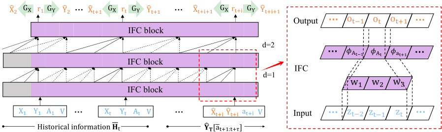
As shown in Figure 2, we propose the Temporal Adaptive Convolutional Intervention Network (TAIN). Following the methodology of [Bai et al., 2018], TAIN consists of a representation module Φ(·), which employs residual connections [He et al., 2016] to concatenate multiple IFC blocks:
When input z and output F(z) dimensions match, B is an identity map. Otherwise, B becomes a 1 × 1 convolution to align dimensions.
TAIN employs an autoregressive recursive strategy [Chevillon, 2007; Taieb and Atiya, 2015] for multi-step prediction, which has also been adopted by [Li et al., 2021; Wang et al., 2024]. During the training process, we need to predict the output and time-varying covariates at the next time step. TAIN defines a feedforward neural network GY to decode the predicted output from the representation Φ(ut).
For notational simplicity, we denote Φ(ut) as rt. We use the Mean Squared Error (MSE) to define the following loss function:
TAIN employs two feedforward neural networks, GX and JX, for covariate prediction. Specifically, GX is responsible for decoding the expected covariates from rt. Drawing inspiration from [Wang et al., 2024], we utilize JX to design a smoothing mechanism. This mechanism, influenced by the gating mechanism in GRUs [Cho et al., 2014], aims to adapt to the varying trends of different covariates. Analogously, we define the following loss function:
where η = Sigmoid(JX(rt)) is the smoothing factor. Following G-formula [Robins, 1986], we estimate the expected outcomes as:
where ¯Lt represents the history of outputs and covariates up to time t. During the prediction phase, we approximate this expectation by sampling the predicted values from Gaussian distributions with means equal to the model predictions and standard deviation σ. Based on Theorem 4.4, we propose the following objective function:
where R(θ) is the regularization term.
5 Experiments
We compare our method against state-of-the-art models for counterfactual estimation over time: RMSN [Lim et al., 2018], CRN [Bica et al., 2020b], G-Net [Li et al., 2021], CT [Melnychuk et al., 2022], ACTIN [Wang et al., 2024], and CTD-NKO [Wang et al., 2025]. To ensure fair comparison, we perform hyperparameter tuning for all baselines (see details in Appendix F), and report RMSE following the standard protocol [Melnychuk et al., 2022] to measure prediction errors against ground-truth counterfactual outcomes.
5.1 Experiments with FS-Tumor data
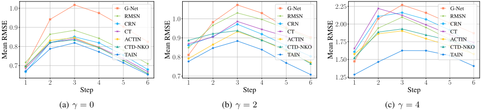
Data. The fully-synthetic tumor (FS-Tumor) growth dataset, constructed using a pharmacokinetic-pharmacodynamic model [Geng et al., 2017], provides a realistic simulation of the combined effects of chemotherapy and radiotherapy on lung cancer patients. This dataset has gained significant attention in the research community and has been extensively utilized for evaluating various causal inference methods in studies such as [Lim et al., 2018; Bica et al., 2020b; Melnychuk et al., 2022; Wang et al., 2024]. One notable feature of this advanced bio-mathematical model is the inclusion of a parameter γ, which allows for the control of time-varying confounding in the dataset. By adjusting the value of γ, researchers can simulate scenarios where historical data have varying degrees of influence on treatment allocation. As γ increases, the confounding bias becomes more pronounced, as past information plays a more dominant role in determining the course of treatment.
| τ = 1 | τ = 2 | τ = 3 | τ = 4 | τ = 5 | τ = 6 | |
|---|---|---|---|---|---|---|
| RMSN | 1.85±0.56 | 3.03±0.76 | 3.50±0.83 | 3.86±0.79 | 4.59±1.44 | 5.21±1.38 |
| CRN | 1.67±0.39 | 2.56±0.78 | 3.07±0.90 | 3.52±0.89 | 4.19±1.53 | 4.77±1.48 |
| G-Net | 2.06±0.54 | 2.92±0.84 | 3.48±1.03 | 3.80±1.01 | 4.42±1.48 | 5.11±1.52 |
| CT | 1.85±0.49 | 2.81±0.83 | 3.30±0.87 | 3.63±0.87 | 4.20±1.35 | 4.85±1.37 |
| ACTIN | 0.89±0.31 | 1.48±0.61 | 1.94±0.69 | 2.58±0.84 | 3.31±1.22 | 4.24±1.83 |
| CTD-NKO | 0.76±0.53 | 1.70±0.87 | 2.28±1.16 | 2.72±1.26 | 3.18±1.59 | 3.95±1.85 |
| TAIN | 0.39±0.10 | 0.60±0.16 | 0.82±0.30 | 1.13±0.40 | 1.31±0.48 | 1.63±0.58 |
In the original dataset, both radiotherapy and chemotherapy interventions are binary. However, in real-world clinical settings, these treatments often involve varying dosages. To better reflect this complexity, we have adapted the interventions to be continuous rather than binary. This modification allows for a more nuanced representation of treatment intensities, aligning our simulations more closely with clinical realities. For a detailed description of the dataset generation process, please refer to Appendix D.
Results. Figure 3 illustrates the performance comparison between TAIN and the baseline models on the FS-Tumor dataset. The results demonstrate that TAIN exhibits superior or highly competitive performance across different levels of time-varying confounding (γ = 0, 2, and 4) and prediction steps (1 to 6 steps). In most cases, TAIN and the baseline models share a similar performance trend, typically reaching a peak RMSE around the 3rd step and then showing a decreasing trend in long-term predictions. It is noteworthy that this trend does not stem from a reduction in the difficulty of long-term prediction tasks, but rather may be attributed to the reduction of tumor size after the application of treatment interventions, leading to a decrease in RMSE.
It is especially important to note that as confounding bias becomes more severe, treatment allocation grows increasingly imbalanced, complicating the capture of temporal treatment interactions. In such scenarios, the benefits of TAIN are pronounced, demonstrating the superiority of its distinctive IFC approach. For more comprehensive experimental results on the FS-Tumor dataset, please refer to Appendix D.
5.2 Experiments with CISDData
Data. The Continuous Intervention Synthetic Dataset (CISD) [Wang et al., 2024] is a synthetic time series dataset designed to simulate the effects of continuous interventions. In this dataset, the generation of treatment variables relies on nonlinear transformations of historical covariate data and the addition of noise, reflecting confounding bias through a Beta distribution. Furthermore, the generation of covariate and outcome variables significantly depends on complex nonlinear transformations that not only capture the dynamic influence of historical covariates and treatment data but also enhance the realism of the dataset. These nonlinear processing techniques make the CISD dataset a useful tool for investigating the intricate dynamic effects of continuous interventions, making it particularly suitable for simulating treatment effects in real-world scenarios. For a detailed description of the dataset generation process, please refer to Appendix D.
| τ = 1 | τ = 2 | τ = 3 | τ = 4 | τ = 5 | τ = 6 | |
|---|---|---|---|---|---|---|
| ACTIN | 1.58 ± 0.47 | 1.86 ± 0.92 | 1.90 ± 1.02 | 1.79 ± 0.97 | 1.69 ± 0.94 | 1.58 ± 0.89 |
| ACTINw/o balancing | 1.58 ± 0.47 | 1.88 ± 0.99 | 1.92 ± 1.06 | 1.79 ± 0.97 | 1.67 ± 0.91 | 1.54 ± 0.84 |
| TAIN | 1.29 ± 0.50 | 1.46 ± 0.65 | 1.63 ± 0.78 | 1.62 ± 0.81 | 1.55 ± 0.81 | 1.41 ± 0.76 |
| TAIN w/o DG | 1.26 ± 0.47 | 1.53 ± 0.70 | 1.69 ± 0.84 | 1.68 ± 0.87 | 1.61 ± 0.87 | 1.47 ± 0.82 |
Results. Table 1 presents the τ-step prediction results on the CISD dataset. Compared to the FS-Tumor dataset, CISD has a higher dimensionality of covariates, resulting in more complex temporal treatment interactions. As the number of prediction steps increases, this complexity leads to greater challenges in making accurate predictions, which can be observed from the performance of different models. The results demonstrate that TAIN consistently outperforms other baseline models across all prediction steps. As the number of prediction steps increases, TAIN shows a clearer advantage over baseline models, demonstrating its effectiveness in capturing temporal treatment interactions through the IFC approach. In contrast, models like ACTIN treat treatments as general inputs, limiting their ability to model nonlinear complexities.
5.3 Ablation Studies
To further investigate the effectiveness of our proposed theory, we conducted an ablation study on the FS-Tumor dataset with γ = 4. We compared the performance of the TAIN model with and without the domain generalization strategy to evaluate the impact of the proposed theory on alleviating confounding bias. To contrast with balancing strategies from the perspective of domain adaptation, we also selected ACTIN as a representative for the ablation experiment.
The ablation study results demonstrate the effectiveness of the domain generalization (DG) strategy in TAIN for addressing confounding bias. As shown in Table 2, TAIN with DG consistently outperforms its counterpart without DG for longer time steps (τ ≥ 2), with improvements ranging from 0.06 to 0.07 across τ = 2 to τ = 6. In contrast, while ACTIN also shows improvements with its balancing component, the gains are relatively smaller compared to TAIN's DG strategy. This comparison highlights that our proposed domain generalization approach is more effective at handling the distribution shift between training and testing phases, particularly when dealing with confounding bias. The superior performance of TAIN can be attributed to its explicit consideration of the unique challenge in counterfactual estimation: the unavailability of target domain distributions during testing, which is directly addressed through our framework. Additional analyses on the SAM radius ρ and the RBF-based treatment representation are provided in Appendix F.
6 Conclusion
In this paper, we propose TAIN for longitudinal counterfactual estimation under confounding bias and temporal complexity. By encoding treatment information into the IFC kernel, TAIN highlights treatment effects and captures temporal treatment interactions. It also mitigates time-varying confounding bias by bounding counterfactual estimation error from a domain generalization perspective. Theoretical and empirical results demonstrate its effectiveness, with future work extending evaluation to real-world datasets.
Ethical Statement
This study requires no institutional ethics approval. All results are based on simulated and publicly available datasets.
Acknowledgments
This research was supported in part by the National Nature Science Foundation of China (No. 62137002, 62406302, 62576327), in part by the Natural Science Foundation of Anhui province (No. 2408085QF195), in part by the USTC Research Funds of the Double First-Class Initiative (Grant No. YD9110002085), in part by the Research Funds of Centre for Leading Medicine and Advanced Technologies of IHM (Grant No. 2025IHM01030), and, in part, by Jinan-NTU Green Technology Research Institute (GreenTRI).
@inproceedings{ijcai2026p454,
  title     = {Counterfactual Estimation via Temporal-Aware Intervention Networks},
  author    = {Wang, Xin and Luo, Chi and Lyu, Shengfei and Wan, Yi and Zhou, Xiren and Wang, Xiangyu and Chen, Huanhuan},
  booktitle = {Proceedings of the Thirty-Fifth International Joint Conference on
               Artificial Intelligence, {IJCAI-26}},
  publisher = {International Joint Conferences on Artificial Intelligence Organization},
  editor    = {Diego Calvanese},
  pages     = {4079--4087},
  year      = {2026},
  month     = {8},
  note      = {Main Track},
  doi       = {10.24963/ijcai.2026/454},
  url       = {https://doi.org/10.24963/ijcai.2026/454},
}
TY - CPAPER TI - Counterfactual Estimation via Temporal-Aware Intervention Networks AU - Wang, Xin AU - Luo, Chi AU - Lyu, Shengfei AU - Wan, Yi AU - Zhou, Xiren AU - Wang, Xiangyu AU - Chen, Huanhuan T2 - Proceedings of the Thirty-Fifth International Joint Conference on Artificial Intelligence, IJCAI-26 PB - International Joint Conferences on Artificial Intelligence Organization PY - 2026 SP - 4079 EP - 4087 DO - 10.24963/ijcai.2026/454 UR - https://doi.org/10.24963/ijcai.2026/454 ER -Copied
Machine-readable versions of this paper, for tools and AI agents:





