
Dual Branch Mutual Teaching for Long-Tailed Partial Label Learning
Proceedings of the Thirty-Fifth International Joint Conference on Artificial Intelligence. Main Track. Pages 4741-4749.
https://doi.org/10.24963/ijcai.2026/528
Keywords
- Machine Learning: Weakly supervised learning
Abstract
In Partial Label Learning (PLL), each instance is associated with a candidate label set, with exactly one label being true. While most studies implicitly assume balanced class distributions, real-world data often exhibit severe class imbalance distributions, leading to the Long-Tailed Partial Label Learning (LT-PLL) problem. In response, prevailing strategies typically manifest the label space to retrieve more tail samples for improved pseudo-label accuracy. However, hard-to-distinguish tail samples can significantly hinder representation learning and, in turn, affect the quality of pseudo-labels. To address this, we propose a novel Distribution-aware Dual-branch Contrastive Learning framework, DEACON, that decouples representation of head and tail labels via a dual-branch mutual-teaching design, enabling disambiguation across different shot-level groups with tailored representations. DEACON comprises two modules: (i)-a instance-balanced branch trained with a vanilla contrastive objective; (ii)-a label-balanced branch trained with a novel reweighted loss that adjusts the contrastive strength through the conditioned von-Mises Fisher density. The two branches mutually teach each other using their pseudo-labels, and we ensemble their predictions to improve overall performance. Extensive experiments on various benchmarks show that our method consistently outperforms state-of-the-art baselines.Code and appendix can be found in https://github.com/YukiNozzzz/DEACON.
- [Briggs et al., 2012] Forrest Briggs, Xiaoli Z. Fern, and Ra- viv Raich. Rank-loss support instance machines for MIML instance annotation. In Proc. of KDD, pages 534-542, 2012.
- [Chen and He, 2021] Xinlei Chen and Kaiming He. Explor- ing simple siamese representation learning. In Proc. of CVPR, pages 15750-15758, 2021.
- [Chen et al., 2018] Ching-Hui Chen, Vishal M. Patel, and Rama Chellappa. Learning from ambiguously labeled face images. IEEE Trans. Pattern Anal. Mach. Intell., pages 1653-1667, 2018.
- [Cour et al., 2011a] Timothee Cour, Ben Sapp, and Ben Taskar. Learning from partial labels. The Journal of Ma- chine Learning Research, pages 1501-1536, 2011.
- [Cour et al., 2011b] Timothée Cour, Benjamin Sapp, and Ben Taskar. Learning from partial labels. J. Mach. Learn. Res., pages 1501-1536, 2011.
- [Deng et al., 2009] Jia Deng, Wei Dong, Richard Socher, Li- Jia Li, Kai Li, and Li Fei-Fei. Imagenet: A large-scale hierarchical image database. In Proc. of CVPR, pages 248- 255, 2009.
- [Du et al., 2023] Fei Du, Peng Yang, Qi Jia, Fengtao Nan, Xiaoting Chen, and Yun Yang. Global and local mix- ture consistency cumulative learning for long-tailed vi- sual recognitions. In Proc. of CVPR, pages 15814-15823, 2023.
- [Feng et al., 2020] Lei Feng, Jiaqi Lv, Bo Han, Miao Xu, Gang Niu, Xin Geng, Bo An, and Masashi Sugiyama. Provably consistent partial-label learning. In Proc. of NeurIPS, 2020.
- [Gunel et al., 2021] Beliz Gunel, Jingfei Du, Alexis Con- neau, and Veselin Stoyanov. Supervised contrastive learn- ing for pre-trained language model fine-tuning. In Proc. of ICLR, 2021.
- [He et al., 2024] Shuo He, Chaojie Wang, Guowu Yang, and Lei Feng. Candidate label set pruning: A data-centric per- spective for deep partial-label learning. In Proc. of ICLR, 2024.
- [Hong et al., 2023] Feng Hong, Jiangchao Yao, Zhihan Zhou, Ya Zhang, and Yanfeng Wang. Long-tailed partial label learning via dynamic rebalancing. In Proc. of ICLR, 2023.
- [Hüllermeier and Beringer, 2006] Eyke Hüllermeier and Jürgen Beringer. Learning from ambiguously labeled examples. Intell. Data Anal., pages 419-439, 2006.
- [Jia et al., 2024] Yuheng Jia, Xiaorui Peng, Ran Wang, and Min-Ling Zhang. Long-tailed partial label learning by head classifier and tail classifier cooperation. In Proc. of AAAI, pages 12857-12865, 2024.
- [Kang et al., 2020] Bingyi Kang, Saining Xie, Marcus Rohrbach, Zhicheng Yan, Albert Gordo, Jiashi Feng, and Yannis Kalantidis. Decoupling representation and classi- fier for long-tailed recognition. In Proc. of ICLR, 2020.
- [Khosla et al., 2020] Prannay Khosla, Piotr Teterwak, Chen Wang, Aaron Sarna, Yonglong Tian, Phillip Isola, Aaron Maschinot, Ce Liu, and Dilip Krishnan. Supervised con- trastive learning. In Proc. of NeurIPS, 2020.
- [Krizhevsky et al., 2009] Alex Krizhevsky, Geoffrey Hinton, et al. Learning multiple layers of features from tiny im- ages. 2009.
- [Liu et al., 2021] Wenpeng Liu, Li Wang, Jie Chen, Yu Zhou, Ruirui Zheng, and Jianjun He. A partial label metric learning algorithm for class imbalanced data. In Proc. of ACML, pages 1413-1428, 2021.
- [Lv et al., 2020] Jiaqi Lv, Miao Xu, Lei Feng, Gang Niu, Xin Geng, and Masashi Sugiyama. Progressive identification of true labels for partial-label learning. In Proc. of ICML, pages 6500-6510, 2020.
- [Lv et al., 2024] Jiaqi Lv, Biao Liu, Lei Feng, Ning Xu, Miao Xu, Bo An, Gang Niu, Xin Geng, and Masashi Sugiyama. On the robustness of average losses for partial- label learning. IEEE Trans. Pattern Anal. Mach. Intell., pages 2569-2583, 2024.
- [Maaten and Hinton, 2008] Laurens van der Maaten and Ge- offrey Hinton. Visualizing data using t-sne. Journal of machine learning research, pages 2579-2605, 2008.
- [Menon et al., 2021] Aditya Krishna Menon, Sadeep Jaya- sumana, Ankit Singh Rawat, Himanshu Jain, Andreas Veit, and Sanjiv Kumar. Long-tail learning via logit ad- justment. In Proc. of ICLR, 2021.
- [Panis and Lanitis, 2014] Gabriel Panis and Andreas Lanitis. An overview of research activities in facial age estima- tion using the FG-NET aging database. In Proc. of ECCV, pages 737-750, 2014.
- [Qiao et al., 2023] Congyu Qiao, Ning Xu, and Xin Geng. Decompositional generation process for instance- dependent partial label learning. In Proc. of ICLR, 2023.
- [Sra, 2012] Suvrit Sra. A short note on parameter approx- imation for von mises-fisher distributions: and a fast im- plementation of I s (x). Comput. Stat., pages 177-190, 2012.
- [Tian et al., 2024] Shiyu Tian, Hongxin Wei, Yiqun Wang, and Lei Feng. Crosel: Cross selection of confident pseudo labels for partial-label learning. In Proc. of CVPR, pages 19479-19488, 2024.
- [Wang and Zhang, 2018] Jing Wang and Min-Ling Zhang. Towards mitigating the class-imbalance problem for par- tial label learning. In Proc. of KDD, pages 2427-2436, 2018.
- [Wang et al., 2021a] Peng Wang, Kai Han, Xiu-Shen Wei, Lei Zhang, and Lei Wang. Contrastive learning based hy- brid networks for long-tailed image classification. In Proc. of CVPR, pages 943-952, 2021.
- [Wang et al., 2021b] Ziqi Wang, Xiaozhi Wang, Xu Han, Yankai Lin, Lei Hou, Zhiyuan Liu, Peng Li, Juanzi Li, and Jie Zhou. CLEVE: contrastive pre-training for event extraction. In Proc. of ACL, pages 6283-6297, 2021.
- [Wang et al., 2022a] Haobo Wang, Mingxuan Xia, Yixuan Li, Yuren Mao, Lei Feng, Gang Chen, and Junbo Zhao. Solar: Sinkhorn label refinery for imbalanced partial-label learning. In Proc. of NeurIPS, 2022.
- [Wang et al., 2022b] Haobo Wang, Ruixuan Xiao, Yixuan Li, Lei Feng, Gang Niu, Gang Chen, and Junbo Zhao. Pico: Contrastive label disambiguation for partial label learning. In Proc. of ICLR, 2022.
- [Wen et al., 2021] Hongwei Wen, Jingyi Cui, Hanyuan Hang, Jiabin Liu, Yisen Wang, and Zhouchen Lin. Lever- aged weighted loss for partial label learning. In Proc. of ICML, pages 11091-11100, 2021.
- [Wu et al., 2024] Dong-Dong Wu, Deng-Bao Wang, and Min-Ling Zhang. Distilling reliable knowledge for instance-dependent partial label learning. In Proc. of AAAI, pages 15888-15896, 2024.
- [Zhang et al., 2017] Chiyuan Zhang, Samy Bengio, Moritz Hardt, Benjamin Recht, and Oriol Vinyals. Understanding deep learning requires rethinking generalization. In Proc. of ICLR, 2017.
- [Zhang et al., 2018] Hongyi Zhang, Moustapha Cissé, Yann N. Dauphin, and David Lopez-Paz. mixup: Beyond empirical risk minimization. In Proc. of ICLR, 2018.
- [Zhang et al., 2022] Fei Zhang, Lei Feng, Bo Han, Tongliang Liu, Gang Niu, Tao Qin, and Masashi Sugiyama. Exploiting class activation value for partial- label learning. In Proc. of ICLR, 2022.
- [Zou et al., 2022a] Ding Zou, Wei Wei, Xian-Ling Mao, Ziyang Wang, Minghui Qiu, Feida Zhu, and Xin Cao. Multi-level cross-view contrastive learning for knowledge- aware recommender system. In Proc. of SIGIR, pages 1358-1368, 2022.
- [Zou et al., 2022b] Ding Zou, Wei Wei, Ziyang Wang, Xian- Ling Mao, Feida Zhu, Rui Fang, and Dangyang Chen. Improving knowledge-aware recommendation with multi- level interactive contrastive learning. In Proc. of CIKM, pages 2817-2826, 2022.
References were extracted automatically from the PDF and may contain errors.
Full text extracted automatically from the PDF; figures, tables and equations may differ. The PDF is the version of record.
1 Introduction
Over the past few decades, the advancement of supervised learning has been largely underpinned by the availability of large-scale, well-annotated datasets such as ImageNet [Deng et al., 2009]. However, acquiring precise labels is difficult. Distinguishing similar classes is labor-intensive and often requires expert-level knowledge that non-experts lack. Such inherent ambiguities are common across various real-world scenarios, ranging from facial age estimation [Panis and Lanitis, 2014] to automatic image annotation [Chen et al., 2018] and bird song recognition [Briggs et al., 2012]. To alleviate the burden of precise annotation, a practical strategy is to assign a set of candidate labels to each sample, giving rise to the Partial Label Learning (PLL) paradigm [Cour et al., 2011b]. By accommodating label uncertainty, PLL is more accessible to non-expert annotators and significantly reduces labeling costs. The core of PLL is label disambiguation-the process of identifying the unique ground-truth label from the ambiguous candidate set. To this end, a plethora of methods have been developed to tackle this problem, including identification-based methods [Lv et al., 2020], averagingbased methods [H¨ullermeier and Beringer, 2006], and datageneration-based methods [Feng et al., 2020].
∗Corresponding author.
Despite their promise, most existing PLL methods are predicated on the assumption that training data follows a class-balanced distribution. However, this assumption is frequently violated in practical applications, where datasets naturally exhibit a long-tailed label distribution [Kang et al., 2020]. This inherent imbalance significantly exacerbates the challenge of label disambiguation, as model predictions tend to be heavily biased toward head classes, leading to severely degenerated performance on tail classes [Wang et al., 2022a]. To address this problem, namely, Long-Tailed Partial Label Learning (LT-PLL), a handful of studies have been proposed, which can be broadly categorized into pseudo-labeling-based methods and ensemble-based methods. Pseudo-labelingbased methods focus on assigning pseudo-labels that simultaneously handle label disambiguation and distribution bias. For instance, SoLar [Wang et al., 2022a] formulates label disambiguation as an optimal transport problem, using an estimated class distribution to mitigate pseudo-labeling bias. Similarly, RECORDS [Hong et al., 2023] dynamically maintains class prototypes for prior estimation and subsequently employs logit-adjustment [Menon et al., 2021] to mitigate the long-tailed effects stemming from the long-tailed distribution. Moving beyond a single classifier, recent advances in ensemble methods underscore the efficacy of multi-classifier frameworks in addressing class imbalance and label ambiguity. A recent work, HTC [Jia et al., 2024], proposes a cooperative ensemble framework that adaptively fuses predictions from specialized dual classifiers via a classifier weight estimation module, thereby mitigating the performance tradeoff between head and tail classes. Nevertheless, these methods typically manifest the label space to refine pseudo-labels, while overlooking the fundamental importance of learning high-quality representations for label disambiguation [Wang et al., 2022b], where hard-to-distinguish tail samples can hinder representation learning and consequently degrade pseudo-label quality.
To mitigate this issue, this paper aims to enhance representation learning for LT-PLL, and propose DEACON, a novel Distribution-awarE DuAl-branch CONtrastive Learning framework. Specifically, to ensure that different shotlevel groups learn effective representations, DEACON adopts a dual-branch design that simultaneously optimizes a headdominant and a tail-focused feature space, yielding tailored representations across shot levels that facilitate more reliable label disambiguation. On one hand, the head-dominant branch employs pseudo-labeling contrastive learning (PseCo) to exploit the abundance of head classes. By enforcing intraclass compactness and inter-class separability under instancebalanced sampling, PseCo provides a robust feature backbone and sharpens decision boundaries. On the other hand, to tackle sample scarcity in the tail-focused branch, we introduce Distribution Estimation Contrastive Learning (DECo), which shifts the paradigm from individual-sample comparisons to distribution-aware modeling. Rather than relying on a few samples within a single batch, DECo captures the overall feature distribution of each class from a global perspective, offering a consistent, low-variance training signal, alleviating the estimation bias of batch-level statistics, and ensuring discriminative representations for rare categories. Once both branches have learned tailored representations, we let them mutually generate pseudo labels for each other and ensemble their predictions to further improve overall performance.
Extensive experiments on several synthetic and real-world benchmarks demonstrate that our method significantly outperforms state-of-the-art methods. e.g., on the CIFAR10-LT, our method improves accuracy by 2.81% on average relative to the best baseline. More impressively, on the PASCAL VOC, our approach yields a notable 6.08% improvement.
2 RelatedWork
Partial Label Learning (PLL). PLL is a prominent weakly supervised learning paradigm in which each training instance is associated with a set of candidate labels that contain the ground truth. Consequently, the fundamental objective of PLL is label disambiguation-identifying the latent true label from the ambiguous candidate set. Existing methods can be categorized into three distinct paradigms: identificationbased, averaging-based, and data-generation-based strategies. Identification-based strategies aim to disambiguate the ground-truth label from the candidate set while concurrently optimizing the classifier [Lv et al., 2020; He et al., 2024; Tian et al., 2024]. Averaging-based strategies assign uniform weights to all candidate labels and use the model's aggregated mean for supervision [H¨ullermeier and Beringer, 2006; Cour et al., 2011a; Lv et al., 2024]. Data-generationbased strategies characterize the generative process from latent ground-truth labels to observed partial label sets, enabling the derivation of loss functions with rigorous theoretical guarantees [Feng et al., 2020; Wen et al., 2021; Qiao et al., 2023]. In addition, numerous studies leverage representation learning paradigms to augment these foundational strategies, incorporating contrastive learning and consistency regularization [Wang et al., 2022b; Wu et al., 2024].
Long-tailed Partial Label Learning (LT-PLL). The literature addressing the LT-PLL problem remains relatively scarce. Early attempts, such as those by [Wang and Zhang, 2018; Liu et al., 2021], primarily addressed this challenge using oversampling techniques and regularization constraints. From an optimization perspective, SoLar [Wang et al., 2022a] formulates label disambiguation as an optimal transport problem and uses the Sinkhorn-Knopp algorithm for efficient approximation. The core objective of SoLar is to mitigate pseudo-label bias by constraining assignments to align with dynamically estimated class distribution priors. Similarly, RECORDS [Hong et al., 2023] introduces a dynamic rebalancing strategy that recovers class priors by maintaining category prototypes and incorporates logit adjustment to calibrate model predictions. To address the inherent performance trade-off between head and tail classes, HTC [Jia et al., 2024] proposes a head and tail classifier cooperation framework. This approach employs a classifier weight estimation module to adaptively fuse predictions.
Contrastive Learning. Contrastive learning has been widely used across domains, leveraging the idea of pulling similar instances together and pushing distinct instances apart. Self-supervised paradigms rely on data augmentation to construct positive pairs from unsupervised data. While self-supervised learning relies on specific strategies to generate positive and negative pairs from unsupervised data [Wang et al., 2021b; Zou et al., 2022a; Zou et al., 2022b], pseudolabeling contrastive learning has been proposed as an extension that explicitly incorporates label information to define these pairs [Khosla et al., 2020; Gunel et al., 2021; Wang et al., 2021a]. Surprisingly, although contrastive learning has proven effective in representation learning, its application to LT-PLL has been overlooked in existing literature.
3 Method
3.1 Preliminary
Let X ∈ Rd denote the d-dimensional feature space and Y = {1, . . . ,K} denote the label space consisting of K classes. We consider a Long-Tailed Partial Label Learning (LT-PLL) dataset D = {(xi, Si)}ni=1 , containing n instances. Each instance xi ∈ X is associated with a set of candidate labels Si ⊆ Y. It is assumed that the unique ground-truth label yi is hidden within the candidate set, satisfying yi ∈ Si.
Let f head (·; θhead ), f tail (·; θtail ) represent the deep feature extractor parameterized by θtail and θhead . The logits produced by the classifiers are formulated as g(f head (x; θhead );W head ), g(f tail (x; θtail );W tail ) where W head , W tail denotes the parameters of the classifier. We define the probability matrix as P ∈ Rn×K , where the probability vector for the i-th instance phead i , ptail i is computed via the softmax function. To facilitate label disambiguation, we maintain pseudo-label matrix Qhead , Qtail , where Q = [q1, . . . , qn]⊤. The entire dataset is defined as Dall. In our work, we use CE loss H(pi, qi) = ∑Kj=1 -qij log pij .
3.2 Distribution-aware Contrastive Representation Learning for LTPLL
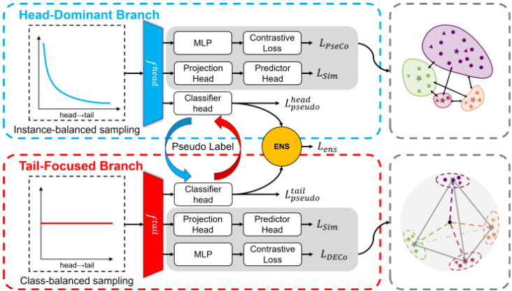
Existing methods primarily focus on refining the label space to improve pseudo-labels, but they often neglect the fundamental necessity of learning high-quality representations for effective label disambiguation. In this context, hard-todistinguish tail samples can hinder representation learning, which in turn degrades the quality of pseudo-labels. In this work, we introduce DEACON, a novel Distribution-awarE DuAl-branch CONtrastive Learning framework, as shown in Figure 1. Specifically, to ensure that different shot-level groups learn effective representations, DEACON adopts a dual-branch design that simultaneously optimizes a headdominant and a tail-focused feature space, yielding tailored representations across shot levels that facilitate more reliable label disambiguation. To achieve this, both branches first map the extracted features into a latent embedding space through a projection head. Within this space, the head-dominant branch is optimized by pseudo-labeling contrastive loss to exploit the abundance of head classes, while for the tail-focused branch, we introduce a distribution estimation contrastive learning objective to alleviate the sample scarcity. Once both branches have acquired tailored representations, they mutually generate pseudo-labels for each other, which effectively mitigates the inherent bias of any single branch toward specific class frequencies. Ultimately, an ensemble module is integrated to leverage the complementary strengths of both feature spaces.
Reliable Resampling
To facilitate the construction of distinct feature representations, DEACON comprises a head-dominant branch and a tail-focused branch, supported by a reliable resampling strategy. This strategy identifies reliable samples prel by leveraging the small-loss criterion, which posits that samples with lower loss values are more likely to be correctly labeled [Zhang et al., 2017]. Specifically, for each class j, we select a fraction of samples based on the ratio πj · α(k), where πj denotes the frequency of class j and α(k) represents a dynamic scaling coefficient at training epoch k. Within this framework, the two branches specialize in different aspects of the data: the head-dominant branch employs instancebalanced sampling (i.e., the natural distribution) to capture global characteristics and robust features; conversely, the tailfocused branch adopts class-balanced sampling (i.e., uniform sampling) to alleviate the bias toward head classes, thereby enhancing the model's discriminative power on the tail distribution. Thus, we can obtain the reliable subset Dhead rel , Dtail rel .
Head-Dominant Branch
We employ pseudo-labeling contrastive learning (PseCo) [Khosla et al., 2020] to explicitly enforce intra-class compactness and inter-class separability. Specifically, the instance-balance sampling strategy adopted in this branch ensures a high frequency of positive pairs for the head classes within each mini-batch. Leveraging this abundance, PseCo can maximize its effectiveness in forming tight, wellseparated clusters for the head-dominant branch, thereby establishing a discriminative and robust feature foundation for the model. Formally, for a anchor sample xi with a refined pseudo-label ˜ yi, we construct its positive set P(i) by identifying other samples xj (and their augmented views) within the current mini-batch that share the same target, i.e., P(i) = {j | ˜ yj = ˜ yi, j ̸= i}. The PseCo loss is then computed to pull these positive pairs together while pushing away other pairs. The loss function is defined as:
where zhead denotes the normalized embedding, T is the temperature parameter, and A(i) is the set of all contrastive candidates. By optimizing LPseCo, the encoder learns to cluster samples of the same class in the hypersphere, effectively distinguishing the ground-truth label from false candidates.
Tail-Focused Branch
For the Tail-Branch, our goal is to construct a class-balanced feature space. Unlike the head-dominant branch, we use a uniform sampling strategy to select high-confidence samples. However, this reduction in data volume poses a significant challenge to representation learning, as the efficacy of PseCo heavily relies on an abundant amount of data. To mitigate the sample scarcity within the tail-focused branch, we move beyond instance-level comparisons and reformulate the contrastive objective from a distributional perspective. Inspired by [Wang et al., 2022b], we explicitly model the feature distribution as a von Mises-Fisher (vMF) mixture distribution. Accordingly, the probability density function for a unit embedding ztail in class j is:
where µj is the mean direction of the class j with ∥µj∥2 = 1, κj ≥ 0 is the class-specific concentration parameter indicating the tightness around µj, I(d/2-1) denotes the modified Bessel function of the first kind at order d/2 - 1, and Cd(κ) is the normalization factor whose computation is described in [Appendix B]. Specifically, we propose the Distribution Estimation Contrastive (DECo) loss, which is formulated as a reweighted loss that adjusts the contrastive strength:
where κ′j = ∥κjµj +ztail /T∥2, T is the temperature parameter that controls the concentration of the distribution. We further prove DECo is an unbiased estimator of PseCo.
Proposition 1. Let P(X, Y ) denote the data distribution where X and Y are random variables, and assume the feature space follows the vMF mixture distribution defined above. We define the instance-level loss functions for PseCo and DECo as: lPseCo(xi, yi) = - 1 |P (i)| ∑j∈P(i) log exp(zi·zj/T) ∑k∈A(i) exp(zi·zk/T)
Under this formulation, the population-level DECo loss is an unbiased estimator of the population-level PseCo loss, i.e.,
To apply this analytical formulation in practical training, we need to estimate the key unknown parameters of the distribution, namely: the mean directions µ and concentration parameters κ for each class. For the mean directions µ, each class has µj = ¯ztail j ∥¯ztail j ∥2 , ¯ztail j is the mean vector updated in a online estimation algorithm:
where ¯ztail′ j is the sample mean of class j in the current batch. mj and nj represent the number of samples in the previous batch and the current batch. Regarding κ, we follow [Sra, 2012] for a simple estimation:
where d is the feature dimension. Once parameters ¯ztail j , µ, and κ are estimated, DECo loss can be computed to supervise the representation learning process, thereby facilitating a more robust and class-balanced feature space.
Mutual Disambiguation
To conduct label disambiguation, we develop a mutual disambiguation mechanism. Specifically, we use each branch's predictions to generate pseudo-labels for the other branch. As the prediction on one epoch may not be reliable, we use the moving average mechanism to build the soft-pseudo label for the head-dominant branch, i.e.
where m ∈ [0, 1] is a predefined scalar and qi denotes the soft-pseudo label vector for xi. To initialize the i-th softpseudo label, we set qhead ij = 1 |Si| to each class j.
For the tail-focused branch, we simply use logit adjustment with the prediction from the head-dominant branch, i.e.
where πy denotes the class frequency vector, and τ > 1 is an adjustment coefficient that strengthens the logit adjustment. We use an online estimation strategy to track the data distribution πy via a moving average mechanism following [Wang et al., 2022a; Jia et al., 2024]. Specifically, we initialize the estimated distribution r as a uniform prior, r = [1/K, . . . , 1/K]. During training, we iteratively refines r by aggregating the predictive signals from the tailfocused branch: r ← mr + (1 - m)πy, where the current epoch's distribution πy is estimated as πj = 1n ∑ni=1 I(j = argmaxj ′∈Si f tail j ′ (xi)).
3.3 Practical Implementation
Self-SimSiam Training. In the context of LT-PLL, supervision signals are doubly compromised: intrinsic label ambiguity acts as noise, while the long-tailed distribution biases pseudo-labels towards head classes. Relying solely on supervised objectives risks learning a degenerated feature space caused by incorrect disambiguation and the long-tailed effect. Thus, we introduce a self-supervised learning branch utilizing SimSiam [Chen and He, 2021] to enforce intrinsic feature consistency. Following the augmentation strategy from GLMC [Du et al., 2023], we generate two distinct views for each input image. Detailed information is provided in [Appendix C]. These views are then fed into the encoder network and a subsequent projection head to extract the latent representations hg and hl. Finally, a prediction head transforms these representations to output to yield the outputs ug and ul. We minimize their negative cosine similarity:
where ∥ · ∥ denotes the l2-norm. To avoid the trivial solution of representation collapse when training without negative samples, we employ the asymmetric stop-gradient strategy as proposed in SimSiam. The loss function is formulated as:
where sg(·) denotes a stop-gradient operator, which means that hg and hl are treated as a constant.
Ensemble Module. To improve overall predictive performance, we use an ensemble module inspired by HTC [Jia et al., 2024] that aggregates outputs from both branches. For a test sample xi, we first feed it into both branches to obtain the predictions phead i and ptail i . Then, the corresponding weights whead and wtail are computed via the ensemble module. These weights represent the relative importance of the specific sample xi, effectively balancing the influence of the two branches. The final ensemble prediction is calculated as pens i = whead · phead i + wtail · ptail i . Finally, the predicted label for xi is obtained by ypred i = argmaxpens i . The ensemble loss is defined as:
Overall Objective Loss. By combining the preliminary loss and the CE loss of reliable samples, we define the classifier loss for both branches. Since the output may not be reliable in the early stages of training, we progressively increase the proportion of the loss contributed by the identified reliable samples, resulting in:
where a dynamic balancing function β(k) = min(k/E, 1), k is the epoch number and E is a preset epoch number.
Furthermore, we integrate distribution-aware contrastive loss, SimSiam loss, and ensemble loss to enhance the quality of the learned representations. Consequently, the final objective functions for each branch are formulated as follows:
where ϕ is a hyperparameter that controls SimSiam loss.
4 Experiment
4.1 Experimental Settings
Datasets. Following the previous works [Wang et al., 2022a; Hong et al., 2023; Jia et al., 2024], we evaluate our method on long-tailed versions of CIFAR10/100 [Krizhevsky et al., 2009] and the real-world dataset PASCAL VOC [Hong et al., 2023]. For the synthetic long-tailed datasets, training samples are subsampled according to an imbalance ratio γ = n1/nC, where the sample count for class j follows nj = n1 · γ- j-1 K-1 . We configure CIFAR10 with n1 = 5000,K = 10 and CIFAR100 with n1 = 500,K =
100. The method is evaluated under varying imbalance ratios: γ ∈ {50, 100, 150, 200, 250} for CIFAR10 and γ ∈ {10, 20, 50, 100, 150} for CIFAR100. Partial labels are generated by flipping negative labels ¯ y ̸= y into the candidate set with probability η. We adopt η ∈ {0.3, 0.5} for CIFAR10 and η ∈ {0.05, 0.1} for CIFAR100.
Baselines. We validate our method against eight baselines, including five state-of-art PLL methods: LW [Wen et al., 2021], CC [Feng et al., 2020], PRODEN [Lv et al., 2020], CAVL [Zhang et al., 2022], and PiCO [Wang et al., 2022b], as well as three specialized LT-PLL approaches: Solar [Wang et al., 2022a], RECORDS [Hong et al., 2023] and HTC [Jia et al., 2024]. For all compared methods, we adopt the hyperparameter configurations specified in their respective original manuscripts to ensure reproducibility and fairness.
Implementation details. We utilized an 18-layer ResNet as the feature backbone for our experiments. The model was trained for 850 epochs with SGD as the optimizer, using a momentum of 0.9 and a weight decay of 0.001. The initial learning rate was set to 0.01, and was divided by 10 after 700 and 800 epochs. We set the batch size to 256 for CIFAR10 and CIFAR100 and 64 for PASCAL VOC. For all methods on PASCAL VOC, we loaded the ImageNet pre-trained weights for the feature extractor to improve training efficiency.
To improve reliability, we use Mixup [Zhang et al., 2018] to enhance the model's memory of the correspondence between labels and features. Detailed information is shown in [Appendix D]. We linearly ramped up the reliable sample ratio α from 0.2 to 0.6 in the first 50 epochs, dynamic balancing coefficient β from 0 to 0.9 in the first 50 epochs for all experiments. When imbalance ratio γ ≥ 200, the logit adjustment coefficient τ was set to 1.8, otherwise, τ = 2. RECORDS is a plug-in approach for PLL to address LT-PLL. We used the best setting provided by the original paper, i.e., CORR+RECORDS+Mixup, for all RECORDS experiments in this paper. All experiments were conducted three times with the same random seed, and the model with the best performance on the validation set was used as the final model.
4.2 Experimental Results
Main Results
Ourmethod achieves optimal results. As presented in Table 1, our proposed method consistently outperforms stateof-the-art methods on both CIFAR10-LT and CIFAR100-LT datasets across all configurations of flipping probability η and imbalance ratio γ. These quantitative results indicate that our approach effectively mitigates the adverse effects of long-tailed distributions and label ambiguity. Specifically, on CIFAR10-LT, we surpass the strongest baseline, HTC, by an average margin of 2.81%, with a maximum improvement of 5.61% under the CIFAR10-LT (η = 0.5, γ = 200) setting. Similar performance gains are observed on the more challenging CIFAR100-LT, where we outperform HTC by 2.10% on average, specifically achieving a 3.28% improvement on CIFAR100 (η = 0.1, γ = 20) setting.
Our method achieves SOTA performance on different class shots. We report classification accuracy across three disjoint groups by sample frequency: Many, Medium, and Few. Table 2 presents the detailed results on CIFAR10-LT (η = 0.5, γ = 100) and CIFAR100-LT (η = 0.1, γ = 20), DEACON consistently outperforms the baselines, demonstrating superior performance. Specifically, on CIFAR10-LT, our method achieves a remarkable accuracy of 83.57% on the Few-shot group, surpassing the second-best HTC by 6.14%. It is worth noting that while traditional PLL methods like PRODEN achieve high accuracy on Many-shot classes, they suffer from severe performance degradation on tail classes. In contrast, our method alleviates this trade-off while maintaining balanced performance across all class groups. The advantage is even more pronounced on the more challenging CIFAR100-LT dataset, where our method dominates all groups. We achieve 79.21% on Many-shot and 46.85% on Few-shot classes, outperforming the second-best method, HTC, by 4.91% and 6.88%, respectively.
| CIFAR10-LT | ||||||||||
|---|---|---|---|---|---|---|---|---|---|---|
| η = 0.3 | η = 0.5 | |||||||||
| Method | γ = 50 | γ = 100 | γ = 150 | γ = 200 | γ = 250 | γ = 50 | γ = 100 | γ = 150 | γ = 200 | γ = 250 |
| LW | 44.51 ± 0.03 | 38.98 ± 3.39 | 41.00 ± 0.34 | 38.58 ± 3.63 | 36.04 ± 3.09 | 24.62 ± 9.67 | 20.22 ± 1.42 | 20.45 ± 0.93 | 19.72 ± 0.58 | 19.99 ± 0.59 |
| CC | 78.76 ± 0.27 | 60.45 ± 1.06 | 54.96 ± 3.54 | 51.87 ± 0.57 | 50.69 ± 0.98 | 73.09 ± 0.40 | 47.64 ± 1.07 | 44.20 ± 0.89 | 43.02 ± 0.42 | 40.22 ± 0.75 |
| PLL PRODEN | 81.95 ± 0.19 | 54.70 ± 1.07 | 51.00 ± 1.45 | 48.49 ± 0.41 | 45.19 ± 1.40 | 66.00 ± 3.60 | 42.90 ± 1.49 | 39.33 ± 0.97 | 38.18 ± 0.87 | 36.77 ± 0.92 |
| CAVL | 37.63 ± 0.28 | 37.00 ± 0.06 | 35.93 ± 0.34 | 35.07 ± 2.2 | 34.03 ± 1.26 | 34.71 ± 0.63 | 31.25 ± 1.99 | 27.81 ± 2.25 | 26.28 ± 0.09 | 27.09 ± 1.01 |
| PiCO | 75.42 ± 0.49 | 72.81 ± 0.37 | 69.29 ± 0.99 | 65.05 ± 1.44 | 64.04 ± 1.45 | 72.33 ± 0.08 | 67.50 ± 2.87 | 62.95 ± 2.83 | 57.55 ± 0.73 | 53.38 ± 3.45 |
| RECORDS | 84.19 ± 0.23 | 77.95 ± 0.36 | 73.63 ± 0.55 | 71.67 ± 0.57 | 66.73 ± 0.68 | 82.15 ± 0.28 | 74.05 ± 1.11 | 67.74 ± 1.30 | 63.75 ± 0.47 | 58.61 ± 2.35 |
| LT-PLL SoLar | 83.80 ± 0.52 | 57.13 ± 1.46 | 47.53 ± 1.22 | 41.94 ± 1.92 | 39.13 ± 0.30 | 81.38 ± 2.84 | 52.56 ± 1.62 | 42.49 ± 0.59 | 36.36 ± 1.48 | 33.81 ± 0.43 |
| HTC | 88.36 ± 0.32 | 84.81 ± 0.08 | 81.87 ± 0.35 | 80.51 ± 0.12 | 78.40 ± 0.62 | 86.11 ± 1.07 | 82.68 ± 0.52 | 79.41 ± 0.81 | 73.49 ± 3.51 | 71.80 ± 1.73 |
| Ours | 89.90 ± 0.03 | 87.02 ± 0.01 | 84.51 ± 0.01 | 82.95 ± 0.20 | 81.15 ± 0.08 | 88.49 ± 0.01 | 85.12 ± 0.15 | 82.85 ± 0.01 | 79.10 ± 0.64 | 74.48 ± 0.49 |
| CIFAR100-LT | ||||||||||
| η = 0.05 | η = 0.1 | |||||||||
| Method | γ = 10 | γ = 20 | γ = 50 | γ = 100 | γ = 150 | γ = 10 | γ = 20 | γ = 50 | γ = 100 | γ = 150 |
| LW | 48.85 ± 2.16 | 36.58 ± 0.48 | 28.93 ± 0.48 | 25.41 ± 0.53 | 23.50 ± 0.86 | 6.10 ± 2.05 | 27.14 ± 0.34 | 22.89 ± 0.72 | 20.06 ± 1.08 | 17.72 ± 0.09 |
| CC | 60.36 ± 0.52 | 41.40 ± 1.34 | 32.92 ± 0.73 | 27.81 ± 0.76 | 25.94 ± 0.25 | 57.91 ± 0.41 | 32.50 ± 1.33 | 26.42 ± 0.84 | 22.68 ± 0.33 | 20.37 ± 1.14 |
| PLL PRODEN | 60.31 ± 0.50 | 38.68 ± 0.18 | 31.80 ± 0.18 | 27.68 ± 0.03 | 24.97 ± 0.03 | 47.32 ± 0.60 | 30.99 ± 0.29 | 24.18 ± 0.07 | 21.69 ± 0.14 | 19.81 ± 0.01 |
| CAVL | 23.49 ± 0.43 | 19.95 ± 0.52 | 16.85 ± 0.47 | 15.20 ± 0.33 | 14.04 ± 0.44 | 16.81 ± 1.07 | 14.89 ± 0.35 | 13.80 ± 0.09 | 13.18 ± 0.08 | 12.97 ± 0.52 |
| PiCO | 54.05 ± 0.37 | 48.25 ± 1.52 | 40.12 ± 0.37 | 35.45 ± 0.85 | 33.09 ± 0.33 | 46.49 ± 0.46 | 39.64 ± 0.71 | 33.75 ± 1.77 | 29.40 ± 0.55 | 28.15 ± 0.52 |
| RECORDS | 64.27 ± 0.16 | 57.60 ± 1.99 | 49.04 ± 1.57 | 43.36 ± 1.95 | 39.83 ± 0.34 | 62.29 ± 0.20 | 54.73 ± 0.80 | 45.47 ± 0.74 | 40.48 ± 0.23 | 37.37 ± 1.21 |
| LT-PLL SoLar | 64.75 ± 0.71 | 57.13 ± 1.46 | 47.53 ± 1.22 | 41.94 ± 1.92 | 39.13 ± 0.30 | 61.82 ± 0.71 | 52.56 ± 1.62 | 42.49 ± 0.59 | 36.36 ± 1.48 | 33.81 ± 0.43 |
| HTC | 66.50 ± 0.08 | 61.06 ± 0.38 | 53.19 ± 0.22 | 47.27± 0.49 | 44.31 ± 0.44 | 64.97 ± 0.25 | 58.82 ± 0.30 | 49.95 ± 0.35 | 44.36 ± 0.51 | 41.45 ± 0.31 |
| Ours | 69.51 ± 0.01 | 64.15 ± 0.12 | 55.60 ± 0.14 | 48.62 ± 0.06 | 45.91 ± 0.06 | 67.97 ± 0.05 | 62.10 ± 0.25 | 51.30 ± 0.10 | 45.82 ± 0.46 | 41.74 ± 0.34 |
| Method | CIFAR10-LT | CIFAR100-LT | ||||||
|---|---|---|---|---|---|---|---|---|
| Overall | Many | Medium | Few | Overall | Many | Medium | Few | |
| LW | 27.33 | 89.09 | 1.52 | 0.00 | 7.16 | 20.80 | 0.86 | 0.00 |
| CC | 64.88 | 94.56 | 65.61 | 34.22 | 51.09 | 73.03 | 52.15 | 28.05 |
| PLL PRODEN | 62.17 | 96.83 | 72.18 | 14.17 | 41.82 | 76.86 | 43.14 | 5.43 |
| CAVL | 37.51 | 82.67 | 16.43 | 0.00 | 18.29 | 48.12 | 2.57 | 0.00 |
| PiCO | 63.25 | 93.33 | 66.14 | 29.30 | 39.80 | 70.75 | 42.42 | 6.14 |
| RECORDS | 67.74 | 88.17 | 71.10 | 35.00 | 54.73 | 76.09 | 45.65 | 8.52 |
| LT-PLL SoLar | 74.16 | 96.50 | 76.01 | 49.34 | 53.03 | 74.33 | 54.09 | 30.62 |
| HTC | 82.46 | 88.53 | 79.40 | 77.43 | 58.48 | 74.30 | 61.09 | 39.97 |
| Ours | 85.63 | 89.25 | 82.87 | 83.57 | 62.68 | 79.21 | 62.35 | 46.85 |
Results on real-world PLL datasets. To further verify the superiority of our method in practical scenarios, we evaluated different methods on the real-world dataset PASCAL VOC.
| Method | Result on PASCAL VOC | |||
|---|---|---|---|---|
| Overall | Many | Medium | Few | |
| LW | 18.70 | 50.75 | 9.93 | 0.00 |
| CC | 35.78 | 68.17 | 28.00 | 15.79 |
| PLL PRODEN | 38.30 | 63.17 | 32.93 | 22.36 |
| CAVL | 30.12 | 57.92 | 26.79 | 9.64 |
| PiCO | 49.05 | 70.50 | 45.79 | 33.93 |
| RECORDS | 59.70 | 68.92 | 68.57 | 42.93 |
| LT-PLL SoLar | 61.83 | 76.33 | 65.64 | 45.57 |
| HTC | 67.45 | 75.83 | 70.36 | 57.36 |
| Ours | 73.53 | 77.25 | 76.21 | 67.64 |
As presented in Table 3, our method consistently outperforms the state-of-the-art baselines. Specifically, our method achieves an overall accuracy of 73.53%, outperforming the second-best comparison method, HTC, by 6.08%. Moreover, on the challenging Few-shot classes, our method outperforms HTC by 10.28%. These results demonstrate that our method superiorly handles the more challenging real-world scenarios while exhibiting exceptional generalization performance.
DEACON learns a more distinguishable representation.
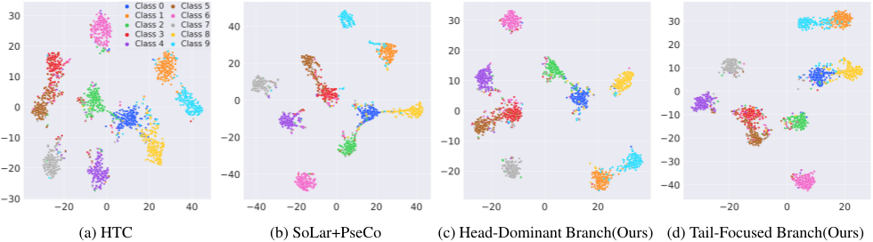
We visualize the feature representations using t-SNE [Maaten and Hinton, 2008] on CIFAR10-LT (η = 0.3, γ = 50) in Figure 2, where colors denote ground-truth labels. We contrast (a) the state-of-the-art method HTC, (b) SoLar with PseCo, and (c, d) our proposed DEACON. (a) HTC exhibits diffuse features and fails to achieve clear class separation. (b) SoLar with PseCo shows a slight improvement but still suffers from significant class overlapping. (c, d) In contrast, DEACON achieves more compact and better-separated clusters, demonstrating its enhanced ability to learn more distinguishable representations than previous methods.
| CIFAR10-LT | ||||
|---|---|---|---|---|
| Method | Overall | Many | Medium | Few |
| Single-Branch | 82.46 | 88.53 | 79.40 | 77.43 |
| Dual-Branch(V1) | 83.75 | 91.55 | 79.60 | 77.50 |
| +SimSiam(V2) | 84.65 | 89.95 | 81.93 | 80.30 |
| +SimSiam+Double PseCo(V3) | 84.80 | 87.65 | 83.13 | 82.67 |
| +SimSiam+Double DECo(V4) | 85.21 | 87.83 | 83.20 | 83.73 |
| +SimSiam+Reverse(V5) | 84.70 | 86.10 | 82.93 | 84.60 |
| +SimSiam+PseCo+DECo(Ours) | 85.78 | 89.82 | 84.50 | 81.67 |
Experimental Analysis
Ablation analysis across DEACON components. We analyze the influence of three key components of our DEACON method, namely Dual-Branch(V1), SimSiam(V2), and Distribution-aware Contrastive learning (Ours). The SingleBranch consists of a standard backbone using dual-head mutual disambiguation, sharing the same encoder with DEACON. As shown in Table 4, the dual-branch architecture improves overall performance by 1.29% on CIFAR10-LT. Specifically, it achieves a 3.02% boost in the "Many" categories compared to the single-branch. Building on this, the integration of SimSiam (V2) further improves overall accuracy to 84.65%. Finally, by incorporating the Distributionaware Contrastive learning (Ours), our method achieves the best performance of 85.78%.
Analysis of contrastive learning variants. We verify the superiority of distribution-aware contrastive learning by comparing it with alternative paradigms. Specifically, we compared our method with three variants:1) V3 by replacing DECo with PseCo; 2) V4 by replacing PseCo with DECo; 3) V5 by reversing them. As shown in Table 4, V3 and V4 yield performance degradations of 0.98% and 0.57%, respectively, indicating that a uniform contrastive paradigm is insufficient to address the joint challenges of class imbalance and label ambiguity. Notably, the reverse variant (V5) significantly reduces 1.08% accuracy, indicating that the distribution-aware weighting must be strictly aligned with the corresponding frequency groups to provide effective guidance.
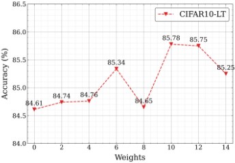
Sensitivity Analysis of ϕ. To investigate the sensitivity of DEACON to the SimSiam weight ϕ, we conduct experiments on CIFAR10-LT by varying ϕ from 0 to 14 with a step of 2. As shown in Figure 3, the accuracy exhibits an upward trend as ϕ increases from 0 to 10, reaching its peak at ϕ = 10. Beyond this point, a slight performance degradation is observed. Specifically, the optimal setting achieves 1.17% improvement over the baseline without the SimSiam component (ϕ = 0). We set ϕ = 10 as the default setting for all experiments.
5 Conclusion
In this paper, we propose DEACON, a novel Distributionaware Dual-branch Contrastive Learning framework. DEACON employs a dual-branch architecture to simultaneously optimize head-dominant and tail-focused feature spaces, thereby yielding tailored representations across different shot-level classes to facilitate reliable label disambiguation. Furthermore, we introduce a distribution contrastive learning module to enhance feature representations. Leveraging these learned features, DEACON performs mutual pseudo-labeling to mitigate class bias and incorporates an ensemble module to exploit the complementary strengths of both branches. Extensive experiments demonstrate that DEACON consistently outperforms existing LT-PLL methods, achieving superior performance and enhanced stability through high-quality feature learning. We hope this work motivates a broader line of research on distribution-aware representation learning for weakly supervised problems under label imbalance.
Acknowledgments
This work is supported by the Ningbo Yongjiang Talent Introduction Programme (No. 2023A-399-G).
@inproceedings{ijcai2026p528,
  title     = {Dual Branch Mutual Teaching for Long-Tailed Partial Label Learning},
  author    = {Ren, Xiangyu and Xia, Mingxuan and Zhu, Guangcheng and Lyu, Gengyu and Wang, Haobo and Lu, Peng},
  booktitle = {Proceedings of the Thirty-Fifth International Joint Conference on
               Artificial Intelligence, {IJCAI-26}},
  publisher = {International Joint Conferences on Artificial Intelligence Organization},
  editor    = {Diego Calvanese},
  pages     = {4741--4749},
  year      = {2026},
  month     = {8},
  note      = {Main Track},
  doi       = {10.24963/ijcai.2026/528},
  url       = {https://doi.org/10.24963/ijcai.2026/528},
}
TY - CPAPER TI - Dual Branch Mutual Teaching for Long-Tailed Partial Label Learning AU - Ren, Xiangyu AU - Xia, Mingxuan AU - Zhu, Guangcheng AU - Lyu, Gengyu AU - Wang, Haobo AU - Lu, Peng T2 - Proceedings of the Thirty-Fifth International Joint Conference on Artificial Intelligence, IJCAI-26 PB - International Joint Conferences on Artificial Intelligence Organization PY - 2026 SP - 4741 EP - 4749 DO - 10.24963/ijcai.2026/528 UR - https://doi.org/10.24963/ijcai.2026/528 ER -Copied
Machine-readable versions of this paper, for tools and AI agents:





